Fluctuating annihilation cross sections and the generation of density perturbations

Abstract

Fluctuations in the mass and decay rate of a heavy particle which for some period dominates the energy density of the universe are known to lead to adiabatic density perturbations. We show that generically the annihilation cross section of the same particle also receives fluctuations, which leads to entropy perturbations at freeze-out. If the particle comes to dominate the energy density of the universe and subsequently decays, this leads to an additional source of adiabatic density perturbations. On the other hand, non-adiabatic density perturbations result when the particle does not decay but contributes to the observed dark matter.

I Introduction

Measurements of the cosmic microwave background radiation cmb1 have revealed a highly uniform energy density background with super-horizon perturbations on the order of one part in $10^{5}$. In the standard inflationary paradigm ref ; infref , these density perturbations were created in the inflationary epoch when quantum fluctuations of the inflaton field expanded beyond the Hubble radius and were converted into density perturbations upon inflaton decay. However, to obtain the observed level of density perturbations from this mechanism requires tight constraints on the inflaton potential cmb2 .

Recently, Dvali, Gruzinov, Zaldarriaga and independently Kofman (DGZK) proposed a new mechanism DGZ for producing density perturbations. A nice feature of their scenario is that the only requirements on the inflaton potential are to produce the required e-foldings of inflation and at a scale consistent with WMAP data. The DGZK mechanism posits the existence of some heavy particle $S$ with a mass and decay rate that depend on the vacuum expectation value of some light field $\chi$. Here $\chi$ is presumed to have acquired super-horizon fluctuations during the inflationary epoch; however $\chi$ never contributes significantly to the energy density of the universe. Nevertheless, the fluctuations in $\chi$ persist and result in fluctuations in the mass and decay rate of $S$, so long as the $\chi$ mass $m_{\chi}$ is less than the Hubble rate $H$ at the time at which fluctuations are transferred to radiation. In the DGZK mechanism the field $S$ comes to dominate the energy density of the universe and decays into radiation while $m_{\chi}<H$. Fluctuations in the mass and decay rate of $S$ result in fluctuations in the duration of $S$ energy domination, which in turn lead to adiabatic density perturbations since the energy of a massive $S$ field redshifts more slowly than that of radiation.

The DGZK mechanism has been studied extensively. For example, the evolution of the density perturbations that result from this mechanism has been studied in detail using gauge invariant formalisms in gaugeinv . These perturbations are shown to possess a highly scale invariant spectrum in scaleinv and are shown to contain significant non-Gaussianities in nongauss . The original DGZK mechanism has also been extended to apply to preheating as studied in extensions . For discussions of the limitations of this mechanism see for example limitations .

In the original DGZK scenario DGZ it is assumed that $S$ decouples while being relativistic. In this paper we generalize this to apply to the case where $S$ freezes-out of equilibrium with a fluctuating annihilation rate $\langle\sigma v\rangle$. We use the term “freeze-out” to refer specifically to the scenario where $S$ decouples from thermal equilibrium after it has become non-relativistic. In this case the number density of $S$ at a temperature $T$ after freeze-out is

$$n_{S} \simeq \frac{T^{3}}{m_{S}m_{\rm pl}\langle\sigma v\rangle}\,,$$ (1)

where $m_{\rm pl}$ is the Planck mass and $m_{S}$ is the mass of $S$. Therefore we expect fluctuations in the mass and annihilation rate of $S$ during freeze-out to result in fluctuations in the number density of $S$. If $S$ lives long enough to dominate the energy density of the universe and subsequently decays, these entropy perturbations are converted into adiabatic perturbations. These add to the ones produced by the original DGZK mechanism and the quantum fluctuations of the inflaton.

This paper is organized as follows. In Section II we describe the density perturbations produced by our generalized DGZK mechanism. Sections III and IV contain explicit models for implementing our mechanism and for producing the fluctuating masses and coupling constants, respectively. Conclusions are given in Section V. In Appendix A an alternate analytical description is given which allows to track the evolution of the perturbations, while in Appendix B Boltzmann equations are derived and solved numerically to confirm the analytical arguments presented in other sections of this paper.

II Analytical determination of the perturbations

Our generalized DGZK mechanism includes a heavy particle $S$ with mass $m_{S}$, decay rate $\Gamma$ and annihilation cross section $\langle\sigma v\rangle$, where $S$ decays to and interacts with radiation. We begin by identifying several key temperature scales. The temperature at which $S$ begins to thermalize with radiation is denoted as $T_{\rm therm}$. We assume for simplicity that $S$ particles are produced only as they thermalize from radiation annihilation below $T=T_{\rm therm}$. We also define:

1. $T_{\rm f.o.}$: Temperature at which $S$ freezes-out of thermal equilibrium;

2. $T_{\rm dom}$: Temperature at which $S$ begins to dominate the energy density of the universe;

3. $T_{\rm dec}$: Temperature at which $S$ decays.

Since the number density of $S$ particles falls off exponentially after $S$ becomes non-relativistic, $T_{\rm f.o.}$ is typically within an order of magnitude of $m_{S}$. Therefore in this paper we always take $T_{\rm f.o.}\simeq m_{S}$. In terms of $m_{S}$, $\Gamma$ and $\langle\sigma v\rangle$ we also find

$$T_{\rm dom} \simeq \frac{1}{m_{\rm pl}\langle\sigma v\rangle}$$

$$T_{\rm dec} \simeq m_{\rm pl}\,\Gamma^{2/3}\langle\sigma v\rangle^{1/3}\,,$$ (2)

where we have assumed $T_{\rm dec}<T_{\rm dom}$ in the last equation. This condition is necessary for significant density perturbations to be produced by this mechanism. In Eq. (2) the cross section is to be evaluated at the freeze-out temperature $T_{\rm f.o.}$. Note that for $S$ particles to be produced in the first place we require $T_{\rm therm}>T_{\rm f.o.}$.

As described in DGZ , the period of $S$ domination between $T_{\rm dom}$ and $T_{\rm dec}$ gives rise to an enhancement of the resulting energy density compared to a scenario where the $S$ domination is absent. Comparing energy densities at common scale factor one finds that after $S$ decays

$$\rho = \left(\frac{\rho_{\rm dom}}{\rho_{\rm dec}}\right)^{1/3}\!\!\!\!\rho_{\rm rad}\,,$$ (3)

where

$$\rho_{\rm dom} \simeq T_{\rm dom}^{4}\,,\qquad\rho_{\rm dec}\,\simeq\,\frac{T_{\rm dec}^{3}}{m_{\rm pl}\langle\sigma v\rangle}\,,$$ (4)

and $\rho_{\rm rad}$ is the energy density which would result without any period of matter domination. As discussed in detail in Section IV, couplings to an additional field $\chi$ can give rise to fluctuations in $m_{S}$, $\Gamma$, and $\langle\sigma v\rangle$:

$$m_{S} = \overline{m}_{S}\left(1+\delta_{m}\right)$$

$$\langle\sigma v\rangle = \langle\overline{\sigma v}\rangle\left(1+\delta_{\langle\sigma v\rangle}\right)$$

$$\Gamma = \overline{\Gamma}\left(1+\delta_{\Gamma}\right)\,,$$ (5)

where the barred quantities refer to background values. According to Eqs. (2-5), these fluctuations give rise to fluctuations in $T_{\rm dom}$ and $T_{\rm dec}$ which result in energy density perturbations

$$\frac{\delta\rho}{\rho} = -\frac{2}{3}\,\delta_{\Gamma}-\frac{4}{3}\,\delta_{\langle\sigma v\rangle}\,.$$ (6)

Note that although $\delta\rho/\rho$ contains no explicit dependence on $\delta_{m}$, both $\delta_{\langle\sigma v\rangle}$ and $\delta_{\Gamma}$ are in general functions of $\delta_{m}$.

Comparing the energy density at a common scale factor corresponds to choosing a gauge where the perturbation in the scale factor vanishes, $\psi=0$. Thus the fluctuation in the energy density computed here can be directly related to the gauge invariant Bardeen parameter bardeen

$$\zeta = -\psi+\frac{\delta\rho}{3(\rho+p)}\,.$$ (7)

Thus we find after $S$ decays

$$\zeta=-\frac{1}{6}\,\delta_{\Gamma}-\frac{1}{3}\,\delta_{\langle\sigma v\rangle}\,.$$ (8)

We can obtain the same result in synchronous gauge, where different regions all have the same global time. Since $\rho\sim 1/t^{2}$ in both matter and radiation dominated universes, one finds that $\delta\rho=0$ on surfaces of constant time. Thus the Bardeen parameter is

$$\zeta = -\psi=\frac{\delta a}{a}\,.$$ (9)

To obtain $\zeta$, we only need to determine $a(t,\Gamma,\langle\sigma v\rangle,m)$ and then compare two regions at fixed $t$, but different $\Gamma$, $\langle\sigma v\rangle$ and $m_{S}$. Assuming the $S$ particles freeze-out while non-relativistic and decay after dominating the energy density of the universe, this gives

$$a(t) = \frac{a(t)}{a(t_{\rm dec})}\frac{a(t_{\rm dec})}{a(t_{\rm dom})}\frac{a(t_{\rm dom})}{a(t_{\rm f.o.})}\frac{a(t_{\rm f.o.})}{a(t_{0})}a(t_{0})$$ (10)

$$= \left(\frac{t}{t_{0}}\right)^{1/2}\left(\frac{t_{\rm dec}}{t_{\rm dom}}\right)^{1/6}a(t_{0})\,,$$

where $t_{\rm dec}\simeq\Gamma^{-1}$ is the time when $S$ decays, $t_{\rm dom}\simeq m^{3}_{\rm pl}\langle\sigma v\rangle^{2}$ is the time at which it dominates the energy density of the universe, and $t_{\rm f.o.}$ is the time at which it freezes-out. Substituting gives

$$a(t) = \left(\frac{t}{t_{0}}\right)^{1/2}m^{-1/2}_{\rm pl}\Gamma^{-1/6}\langle\sigma v\rangle^{-1/3}a(t_{0})\,.$$ (11)

Using this result and Eq. (9) we again obtain Eq. (8).

The above discussion is approximate and requires that $S$ completely dominates the energy density of the universe. Obtaining the perturbations when $S$ does not dominate requires that we include the matter contribution to the scale factor or energy density during radiation domination. This is done in Appendix A using a different formalism. In Appendix B we confirm these analytic results using a numerical calculation of the density perturbations using Boltzmann equations.

III Explicit Models for Coupling $S$ to Radiation

It is important to verify that models exist which exhibit the features discussed in the previous section. We present two models in which the annihilation cross section is determined by renormalizable and non-renormalizable operators, respectively.

The first model is given by the Lagrangian

$${\cal L} = \sqrt{-g}\left[\frac{(\partial_{\mu}S)^{2}}{2}+\frac{(\partial_{\mu}X)^{2}}{2}-\frac{m_{S}^{2}}{2}S^{2}-\frac{m_{X}^{2}}{2}X^{2}\right.$$ (12)

$$\hskip 42.67912pt\left.-\frac{g\,m_{S}}{2}\,S\,X^{2}-\frac{\lambda}{4}\,S^{2}X^{2}\right]\,.$$

We assume that $X$ is in thermal equilibrium with the remaining radiation and that $S$ particles are only produced through their coupling to $X$. The interaction terms in the above model yield an $S$ decay rate and cross section

$$\Gamma \sim g^{2}m_{S}\,,\qquad\langle\sigma v\rangle\,\sim\,\frac{\lambda^{2}}{M^{2}}\,,$$ (13)

where

$$M \simeq \left\{\begin{array}[]{ll}T&\,{\rm when}\,\,\,T\,>\,m_{S}\\ m_{S}&\,{\rm when}\,\,\,T\,<\,m_{S}\end{array}\right.\,.$$ (16)

Note that we neglect the ${\cal O}(g^{4})$ contribution to the cross section. This is justified given the limits on the coupling constants derived below.

The requirement that $T_{\rm therm}>m_{S}$ and that $S$ remains in thermal equilibrium down to $T\simeq m_{S}$ gives the condition on the coupling $\lambda$

$$\lambda > \sqrt{\frac{m_{S}}{m_{\rm pl}}}\,.$$ (17)

On the other hand the condition $T_{\rm dec}<T_{\rm dom}$ implies

$$g^{2}\lambda^{4} < \frac{m_{S}^{3}}{m_{\rm pl}^{3}}\,.$$ (18)

Thus a necessary (but not sufficient) condition on $g$ to satisfy both Eq. (17) and Eq. (18) is

$$g < \sqrt{\frac{m_{S}}{m_{\rm pl}}}\,.$$ (19)

Finally, we require that the period of $S$ domination does not disrupt big bang nucleosynthesis (BBN). Thus the decay of $S$ must reheat the universe to a temperature $T_{\rm rh}>T_{\rm BBN}$, where $T_{\rm rh}\simeq\sqrt{\Gamma m_{\rm pl}}$. This gives

$$g^{2} > \frac{T_{\rm BBN}^{2}}{m_{S}m_{\rm pl}}\,.$$ (20)

Using $T_{\rm BBN}\simeq 10^{-21}m_{\rm pl}$, the above relations provide the constraint $m_{S}\gtrsim 10^{-21}m_{\rm pl}$. Given any $m_{S}$ satisfying this constraint, limits on $\lambda$ and $g$ are calculated using Eq. (17) and Eq. (18).

Note that in this model the $S$ particles are produced at $T=T_{\rm therm}$ and remain in thermal equilibrium with the radiation until they freeze-out at $T\simeq m_{S}$. This is different from the assumption made in DGZ , where $S$ starts in thermal equilibrium and decouples while still relativistic. In order to achieve this scenario, the coupling of $S$ to radiation has to proceed via a higher dimensional operator, or in other words via the propagation of an intermediate particle with mass much greater than $m_{S}$.

This brings us to our second model. Consider a heavy fermion $\psi_{S}$ and a light fermion $\psi_{X}$, coupled via an additional heavy scalar $\phi_{H}$ with mass $m_{H}$,

$${\cal L}_{\rm int}=g_{S}\,\bar{\psi}_{S}\psi_{S}\,\phi_{H}+g_{X}\,\bar{\psi}_{X}\psi_{X}\,\phi_{H}\,.$$ (21)

We also assume that the fermion $\psi_{S}$ decays to radiation with rate $\Gamma$. The annihilation cross section is given by

$$\langle\sigma v\rangle\sim\frac{g_{S}^{2}g_{X}^{2}}{m_{H}^{4}}M^{2}\,,$$ (22)

where $M$ is defined in Eq. (16). In this case, thermalization occurs for temperatures bounded by

$$m_{S}\left(\frac{m_{H}^{4}}{m_{S}^{3}m_{\rm pl}}\frac{1}{g_{S}^{2}g_{X}^{2}}\right)^{1/3}<T<g_{S}^{2}g_{X}^{2}m_{\rm pl}\,.$$ (23)

The conditions that $S$ is in in thermal equilibrium when it reaches $T\simeq m_{S}$ gives the condition

$$g_{S}^{2}g_{X}^{2}>\frac{m_{H}^{4}}{m_{S}^{3}m_{\rm pl}}\,.$$ (24)

Note that one still needs to have a decay rate that is small enough such that $\psi_{S}$ decays after it dominates the universe. The point of this second example is to show that in non-renormalizable models the heavy species can either decouple while non-relativistic or while relativistic, depending on whether Eq. (24) is satisfied or not.

IV Models for producing the fluctuations

The density perturbations in the DGZK mechanism and our generalization originate in fluctuations in a light scalar field $\chi$. In this section we write down explicit models for couplings between $S$ and $\chi$. The reason for doing this is that these interactions can give rise to back reactions which can constrain the magnitude of the produced density perturbations. Similar results hold for couplings between $\psi_{S}$ and $\chi$.

We find it convenient to define $\delta\chi\equiv\chi-\langle\chi\rangle$. Note that this does not correspond to a perturbative expansion. The fluctuations in $\chi$ are created during the inflationary era with $\delta\chi\sim H_{\rm inf}$. Then the leading order equation of motion for $\chi$ can be split into homogeneous and inhomogeneous parts,

$$\langle\ddot{\chi}\rangle = -3H\langle\dot{\chi}\rangle-\langle V^{\prime}\rangle\,,$$

$$\delta\ddot{\chi} = -3H\delta\dot{\chi}+4\dot{\phi}\langle\dot{\chi}\rangle-\delta V^{\prime}-2\phi\langle V^{\prime}\rangle\,.$$ (25)

Here $\delta V^{\prime}\equiv V^{\prime}-\langle V^{\prime}\rangle$, where $V$ is the potential of $\chi$ and the prime denotes a derivative with respect to $\chi$. Also, $\phi$ is the time perturbation in conformal Newtonian gauge. The terms proportional to $\phi$ enter into the leading order equation of motion for $\delta\chi$ because their homogeneous coefficients do not.

To simplify the analysis, we first consider the scenario where $\langle\chi\rangle$ is negligible. From Eqs. (25) we see this is the case when $\langle\chi\rangle<\delta\chi$. Thus we require the equation of motion for $\langle\chi\rangle$ to be Hubble friction dominated for $\langle\chi\rangle<\delta\chi$. This gives the condition

$$H^{2}\delta\chi > H^{2}\langle\chi\rangle\,\,>\,\,\langle V^{\prime}\rangle\,.$$ (26)

The fluctuations $\delta\chi$ persist so long as the equation of motion for $\delta\chi$ is Hubble friction dominated. With $\langle\chi\rangle<\delta\chi$ this translates into the condition

$$H^{2}\delta\chi > \delta V^{\prime}+2\phi\langle V^{\prime}\rangle\,.$$ (27)

Note that we can combine our simplifying condition that $\langle\chi\rangle$ be negligible, Eq. (26), with the condition that the fluctuations in $\delta\chi$ be Hubble friction dominated, Eq. (27). Adding these two equations and dropping factors of 2 this gives the single condition

$$H^{2}\delta\chi > V^{\prime}\,.$$ (28)

We consider the constraints this condition imposes on models for transferring $\chi$ fluctuations to the radiation. We first consider the renormalizable interactions

$${\cal L}_{\chi} = \sqrt{-g}\left[-\frac{\alpha_{S}}{4}S^{2}\chi^{2}-\frac{\mu_{S}}{2}S^{2}\chi\right]\,,$$ (29)

and neglect any couplings between $\chi$ and $X$ as they are irrelevant to our mechanism. When $\chi$ fluctuates these interactions result in $S$ mass fluctuations of

$$\delta_{m} = \frac{\alpha_{S}\delta\chi^{2}}{4m_{S}^{2}}+\frac{\mu_{S}\delta\chi}{2m_{S}^{2}}$$ (30)

$$\sim \sqrt{\left(\frac{\alpha_{S}H_{\rm inf}^{2}}{m_{S}^{2}}\right)^{2}\!\!+\left(\frac{\mu_{S}H_{\rm inf}}{m_{S}^{2}}\right)^{2}}\,,$$

where in the second line we have estimated the size of the rms fluctuation at two widely separated co-moving points. This mass fluctuation gives rise to fluctuations in the decay rate and the annihilation cross section of $S$ according to the mass dependence of Eqs. (13).

As described above, for this fluctuation to persist and for $\langle\chi\rangle$ to remain negligible requires that $H^{2}\delta\chi>V^{\prime}$. Although we assume the self interaction of $\chi$ is always negligible, the interactions of ${\cal L}_{\chi}$ contribute to $V$ and provide the constraint

$$H^{2}\delta\chi > \left(\frac{\alpha_{S}}{2}\delta\chi+\frac{\mu_{S}}{2}\right)\langle S^{2}\rangle\,,$$ (31)

where $\langle S^{2}\rangle$ is evaluated in the thermal bath. This constraint is tightest at $T=m_{S}$ when $\langle S^{2}\rangle/H^{2}\sim m_{\rm pl}^{2}/m_{S}^{2}$. Thus we obtain the constraints

$$\alpha_{S} < \frac{m_{S}^{2}}{m_{\rm pl}^{2}}\,,\qquad\mu_{S}\,\,<\,\,\frac{m_{S}^{2}}{m_{\rm pl}^{2}}H_{\rm inf}\,.$$ (32)

The constraints of Eqs. (32) provide the same upper bound to both terms in Eq. (30). Thus the back reactions of ${\cal L}_{\chi}$ limit the level of density perturbations produced via this mechanism to

$$\zeta \sim \delta_{m}\,<\,\frac{H_{\rm inf}^{2}}{m_{\rm pl}^{2}}\,\lesssim\,10^{-8}\,,$$ (33)

where the last limit on $H_{\rm inf}/m_{\rm pl}$ is measured by the WMAP collaboration cmb2 .

The fluctuations resulting from the second interaction in ${\cal L}_{\chi}$ are linear in $\delta\chi$ and are therefore predominantly Gaussian in their distribution. Since the observed level of Gaussian fluctuations sets $\zeta\sim 10^{-5}$, this interaction cannot provide a significant fraction of the observed density perturbations. However, the fluctuations resulting from the first term in ${\cal L}_{\chi}$ are quadratic in $\delta\chi$ and therefore non-Gaussian extensions . Recent analysis cmb3 limits the amplitude of non-Gaussian perturbations to about $10^{-8}$. Thus we see our model can provide non-Gaussian perturbations right at the limit of current observation. A lower level of perturbations is obtained by reducing $\alpha_{S}$ or $\mu_{S}$.

As a variant on the above scenario, we next consider the non-renormalizable couplings

$${\cal L}^{\prime}_{\chi} = \sqrt{-g}\left[-\frac{\lambda}{4}\,\frac{\chi^{2}}{M_{1}^{2}}\,S^{2}X^{2}-\frac{\lambda}{4}\,\frac{\chi}{M_{2}}S^{2}X^{2}\right]\,.$$ (34)

When $\chi$ fluctuates these interactions result in fluctuations in $\langle\sigma v\rangle$

$$\delta_{\langle\sigma v\rangle} = \frac{2\delta\chi^{2}}{M_{1}^{2}}+\frac{2\delta\chi}{M_{2}}\,\sim\,\sqrt{\left(\frac{H_{\rm inf}^{2}}{M_{1}^{2}}\right)^{2}\!\!+\left(\frac{H_{\rm inf}}{M_{2}}\right)^{2}}.\quad$$ (35)

As above, we require that Eq. (28) be satisfied. For the interactions of ${\cal L}^{\prime}_{\chi}$ this gives

$$H^{2}\delta\chi > \frac{\lambda}{4}\left(\frac{2\delta\chi}{M_{1}^{2}}+\frac{1}{M_{2}}\right)\langle S^{2}X^{2}\rangle\,.$$ (36)

As in the previous example, this constraint is tightest at $T=m_{S}$ when $\langle S^{2}X^{2}\rangle/H^{2}\sim m_{\rm pl}^{2}$. Therefore we find

$$\frac{1}{M_{1}^{2}} < \frac{1}{\lambda}\frac{1}{m_{\rm pl}^{2}}\,,\qquad\frac{1}{M_{2}}\,\,<\,\,\frac{1}{\lambda}\frac{H_{\rm inf}}{m_{\rm pl}^{2}}\,.$$ (37)

Analogous to the previous example, the constraints of Eqs. (37) provide the same upper bound to both terms in Eq. (35). Thus the back reactions of ${\cal L}^{\prime}_{\chi}$ limit the level of density perturbations produced via this mechanism to

$$\zeta \sim \delta_{\langle\sigma v\rangle}\,<\,\frac{1}{\lambda}\frac{H_{\rm inf}^{2}}{m_{\rm pl}^{2}}\,.$$ (38)

This bound is significantly weaker than the bound of Eq. (33) obtained via a fluctuating $S$ mass. For example, the fluctuations resulting from ${\cal L}^{\prime}_{\chi}$ could form the dominant contribution to the observed density perturbations if $\lambda$ is sufficiently small. In addition, for a given $\zeta$ decreasing $\lambda$ allows for a lower scale of inflation. Constraints on the smallness of $\lambda$ are discussed in Section III. Of course, a lower level of Gaussian (non-Gaussian) perturbations is obtained by increasing $M_{2}$ ($M_{1}$).

Above we have taken $\langle\chi\rangle$ to be negligible, which corresponds to taking $\langle\chi\rangle<\delta\chi$. Although this simplifies the presentation, it unnecessarily strengthens the constraints on $\mu_{S}$ and $M_{2}$. We know from Eq. (26) that

$$\langle\chi\rangle>\frac{\langle V^{\prime}\rangle}{H^{2}}\,,$$ (39)

therefore keeping $\langle\chi\rangle$ small implies constraints on the potential $V$. Referring to the second of Eqs. (25), we see that for arbitrary $\langle\chi\rangle$ the requirement that $\delta\chi$ remains Hubble friction dominated gives

$$H^{2}\delta\chi\,>\,\dot{\phi}\langle\dot{\chi}\rangle\,,\quad H^{2}\delta\chi\,>\,\delta V^{\prime}\,,\quad H^{2}\delta\chi\,>\,\phi\langle V^{\prime}\rangle\,.\,\,$$ (40)

The first condition provides the constraint $\langle\chi\rangle<\delta\chi/\phi$, with the evolution of $\phi\sim\zeta$ described in Appendix A. It is sufficient to take $\phi\sim 10^{-5}$, which also ensures that the homogeneous correction that $\langle\chi\rangle$ provides to $m_{S}$ does not change $m_{S}$ by more than order unity. Through an analysis analogous to that above, we find the conditions of Eqs. (40) constrain the level of Gaussian fluctuations for the respective interactions of ${\cal L}_{\chi}$ and ${\cal L}^{\prime}_{\chi}$ to

$$\zeta_{\rm g}\,<\,\frac{\langle\chi\rangle}{\delta\chi}\frac{H_{\rm inf}^{2}}{m_{\rm pl}^{2}}\,,\quad\zeta_{\rm g}\,<\,\frac{1}{\lambda}\frac{\langle\chi\rangle}{\delta\chi}\frac{H_{\rm inf}^{2}}{m_{\rm pl}^{2}}\,;\quad\frac{\langle\chi\rangle}{\delta\chi}\,<\,\frac{1}{\phi}\,.$$ (41)

The additional factor of $\langle\chi\rangle/\delta\chi$ significantly weakens both bounds on Gaussian perturbations. This allows for greater freedom in choosing $\mu_{S}$, $M_{2}$, $\lambda$, and/or $H_{\rm inf}$.

Non-Gaussian perturbations originate from the couplings quadratic in $\chi$. Taking these into account the fluctuation resulting from ${\cal L}_{\chi}$ becomes

$$\zeta\sim\delta_{m}=\frac{\alpha_{S}\delta\chi^{2}}{4m_{S}^{2}}+\frac{\alpha_{S}\langle\chi\rangle\delta\chi}{2m_{S}^{2}}+\frac{\mu_{S}\delta\chi}{2m_{S}^{2}}\,.$$ (42)

Note that the quadratic term $\sim\alpha_{S}$ also gives rise to a Gaussian contribution to $\zeta$. Thus, the non-Gaussian perturbations obey the relation

$$\zeta_{\rm ng}\sim\frac{\alpha_{S}\,\delta\chi}{\mu_{S}+\alpha_{S}\langle\chi\rangle}\zeta_{\rm g}\,.$$ (43)

Note that taking $\alpha_{S}\to 0$ the non-Gaussian fluctuations can be made arbitrarily small. However, even if the $\alpha_{S}$ term in the potential dominates, the non-Gaussian fluctuations are always limited by

$$\zeta_{\rm ng}<\frac{H_{\rm inf}^{2}}{m_{\rm pl}^{2}}\,,$$ (44)

as can be seen by combining Eqs. (41) and (43). As mentioned before, WMAP sets the limit $H_{\rm inf}^{2}/m_{\rm pl}^{2}\lesssim 10^{-8}$ cmb2 , thus the non-Gaussian fluctuations are at or below the current limits from WMAP cmb3 . In addition, the observed Gaussian fluctuations can be produced by choosing $\delta\chi/\langle\chi\rangle$ appropriately. The second model with Lagrangian given in Eq. (34) is less constrained since the factor of $\lambda$ weakens the constraint on $\delta\chi/\langle\chi\rangle$.

V Conclusions

In DGZ it was shown that fluctuations in the mass and the decay rate of a heavy particle $S$, which at some point dominates the energy density of the universe, lead to adiabatic density perturbations. In this scenario it was assumed that the heavy particle decouples from radiation while it is still relativistic.

In this work we have shown that if the heavy particle remains in thermal equilibrium until it becomes non-relativistic, fluctuations in the annihilation cross section of this particle with radiation lead to additional sources of perturbations. We have presented two simple toy models illustrating this effect. These additional fluctuations are generic, unless the annihilation cross section is mediated by an additional particle with mass exceeding $m_{S}$. If the $S$ particle is stable, for example if $S$ is dark matter, then the resulting perturbations are non-adiabatic.

A simple analytical calculation determines the size of the density perturbations from fluctuations in the mass, decay rate and annihilation cross section. The fluctuations due to variations in the annihilation cross section are shown to be of similar size as the ones generated from the original DGZK mechanism. These results are checked numerically using Boltzmann equations in conformal Newtonian gauge in Appendix B.

Appendix A Evolution of Density Perturbations

In this appendix we determine the evolution of density perturbations generated by a fluctuating cross section or mass during freeze-out. Unlike other analytic derivations given elsewhere in this paper, the one provided here allows us to easily follow the growth of the non-adiabatic perturbation during the radiation dominated era after freeze-out. We work in conformal Newtonian gauge with negligible anisotropic stress and use the line element

$$ds^{2}=a^{2}\left[-(1+2\phi)d\eta^{2}+(1-2\psi)\delta_{ij}dx^{i}dx^{j}\right]\,,$$ (45)

with $\psi=\phi$. We track the evolution of perturbations using the gauge invariant entropy perturbation ${\cal S}$ and curvature perturbation $\zeta$.

We will assume that the scattering and annihilation interactions between $S$ and the radiation conserve total particle number. This allows us to obtain a first integral of the Boltzmann equations. Conservation of total particle number in a fixed co-moving volume implies for the entropy perturbation

$${\cal S}\equiv\delta_{S}-\delta_{R}=-\left(\delta_{R}-3\phi\right)\left(1+\frac{n_{R}}{n_{S}}\right)+\frac{\lambda_{0}}{n_{S}a^{3}}\,,$$ (46)

where $\delta_{S}\equiv\delta n_{S}/n_{S}$ and $\delta_{R}\equiv\delta n_{R}/n_{R}$ are the perturbations in the number densities of $S$ and radiation, respectively. Here $\lambda_{0}$ is an integration constant which vanishes in the absence of initial adiabatic perturbations.

Eq. (46) has a few salient features that we now discuss. First note that it admits an adiabatic solution ${\cal S}=0$ whenever both $n_{R}/n_{S}$ and $n_{S}a^{3}$ are constant. This solution is the familiar $\delta_{S}=\delta_{R}=3\phi+{\rm constant}$, with the constant fixed by $\lambda_{0}$. During freeze-out, however, the conditions described above are not satisfied, and entropy perturbations ${\cal S}^{\rm f.o.}$ are generated at that time. Using Eq. (1) we find

$${\cal S^{\rm f.o.}}\simeq-\delta_{\langle\sigma v\rangle}-\delta_{m}~{}.$$ (47)

After freeze-out the heavy particle no longer interacts with the radiation and therefore both $\delta_{S}$ and $\delta_{R}$ obey the perturbed Einstein field equation $\dot{\delta}_{S,R}=3\dot{\phi}$. This is trivially integrated to give

$$\delta_{S,R}=3\phi+\delta_{S,R}^{\rm f.o.}-3\phi^{\rm f.o.}\,.$$ (48)

Thus, after freeze-out the entropy perturbation remains constant ${\cal S}={\cal S}^{\rm f.o.}$.

To derive the evolution of the curvature perturbation $\zeta$, we use Eq. (7) together with $\delta\rho_{S}=\rho_{S}(\delta_{S}+\delta_{m})$ and $\delta\rho_{R}=(4/3)\rho_{R}\delta_{R}$ to find after several lines of algebra

$$\zeta\simeq\frac{\rho_{S}({\cal S}^{\rm f.o.}+\delta_{m})}{3\rho_{S}+4\rho_{R}}+\frac{1}{3}\left(\delta_{R}^{\rm f.o}-3\phi^{\rm f.o.}\right)\,.$$ (49)

Using Eq. (46), the second term on the right is suppressed by $(n_{S}/n_{R})(4\rho_{R}/\rho_{S}+3)$ compared to the first term and is subsequently neglected. We see that in the radiation dominated era the curvature perturbations produced during freeze-out are suppressed relative to the entropy perturbations.

Once the the heavy particle starts to dominate the energy density of the universe, we find

$$\zeta\simeq-\frac{1}{3}\delta_{\langle\sigma v\rangle}\,,$$ (50)

in agreement with the results obtained in the main body of this paper. If $S$ is the dark matter, such a large ratio of entropy to curvature perturbations is disfavored by data, which requires $|{\cal S}/\zeta|\lesssim 1/3$ cmb2 . If instead $S$ decays, the entropy perturbations in $S$ are transferred to radiation. The resulting curvature perturbation is then

$$\zeta\simeq-\frac{1}{3}\delta_{\langle\sigma v\rangle}-\frac{1}{6}\delta_{\Gamma}~{}.$$ (51)

Here we have finally included the effect of inhomogeneous $S$ decay, which are formally calculated in DGZ ; gaugeinv .

Appendix B Numerical Results

We now solve for the evolution of density perturbations during freeze-out using Boltzmann equations (see for example ref ; MB ). As above, we work in conformal Newtonian gauge and consider only super-horizon perturbations, neglecting all spatial gradients next to conformal time derivatives. Since we assume that $S$ is non-relativistic, the distribution function for $S$ is

$$f_{S}=e^{\mu/T}f_{\rm eq}\,,$$ (52)

where $f_{\rm eq}$ is the Maxwell-Boltzmann equilibrium distribution function. Then integrating the background Boltzmann equations over all of phase space gives

$$\dot{n}_{S}+3{\cal H}n_{S} = a\langle\overline{\sigma v}\rangle\left(n_{\rm eq}^{2}-n_{S}^{2}\right)-a\overline{\Gamma}n_{S}$$

$$\dot{n}_{R}+3{\cal H}n_{R} = -\,a\langle\overline{\sigma v}\rangle\left(n_{\rm eq}^{2}-n_{S}^{2}\right)+a\overline{\Gamma}n_{S}\,.$$ (53)

where dots denote derivatives with respect to conformal time, ${\cal H}=\dot{a}/a$ and $n_{\rm eq}$ is the equilibrium number density of $S$ particles. To describe the evolution of the scale factor we use Einstein’s field equation,

$${\cal H}^{2} = \frac{a^{2}}{3m_{\rm pl}^{2}}\left(\rho_{R}+\rho_{S}\right).$$ (54)

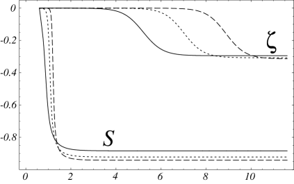
Figure 1: Evolution of ${\cal S}$ and $\zeta$ in units of $\delta_{\langle\sigma v\rangle}$ as a function of $\log(m_{S}/T)$. The solid, dotted and dashed curves correspond to $\langle\sigma v\rangle m_{S}m_{\rm pl}=10^{5}$, $10^{7}$ and $10^{9}$, respectively. The large values of $\langle\sigma v\rangle m_{S}m_{\rm pl}$ are necessary to ensure that the heavy particle is in thermal equilibrium at $T_{0}=m_{S}/4$.

To derive the subleading order Boltzmann equations we allow for fluctuations in $m_{S}$, $\langle\sigma v\rangle$ and $\Gamma$ as defined in Eqs. (5). Note that the resulting fluctuations in the number density of the radiation $\delta_{R}$ correspond to temperature fluctuations $\delta_{T}=\delta_{R}/3$. Therefore the equilibrium number density of $S$ particles acquires fluctuations

$$\delta_{\rm eq}=\frac{3}{2}\left(\delta_{m}+\delta_{T}\right)+\exp\left[-\frac{m_{S}}{T}(\delta_{m}-\delta_{T})\right]-1\,.$$ (55)

When the subleading Boltzmann equations are integrated over all phase space we obtain

$$\dot{\delta}_{S}-3\dot{\phi} = a\langle\overline{\sigma v}\rangle\frac{n_{\rm eq}^{2}}{n_{S}}\left(\phi+\delta_{\langle\sigma v\rangle}+2\delta_{\rm eq}-\delta_{S}\right)$$

$$-\,a\langle\overline{\sigma v}\rangle n_{S}\left(\phi+\delta_{\langle\sigma v\rangle}+\delta_{S}\right)-a\overline{\Gamma}\left(\phi+\delta_{\Gamma}\right)$$

$$\dot{\delta}_{R}-3\dot{\phi} = -\,a\langle\overline{\sigma v}\rangle\frac{n_{\rm eq}^{2}}{n_{R}}\left(\phi+\delta_{\langle\sigma v\rangle}+2\delta_{\rm eq}-\delta_{R}\right)$$ (56)

$$+\,a\langle\overline{\sigma v}\rangle\frac{n_{S}^{2}}{n_{R}}\left(\phi+\delta_{\langle\sigma v\rangle}+2\delta_{S}-\delta_{R}\right)$$

$$+\,a\overline{\Gamma}\frac{n_{S}}{n_{R}}\left(\phi+\delta_{\Gamma}+\delta_{S}-\delta_{R}\right)\,.$$

Note that in deriving the Boltzmann equations we assumed $\delta_{\rm eq}\ll 1$. This ceases to be valid once $T\lesssim m_{S}(\delta_{m}-\delta_{T})$. In this case, however, the factor of $n_{\rm eq}^{2}$ in front of the terms containing $\delta_{\rm eq}$ is exponentially suppressed compared to the remaining terms.

The independent perturbations in Eqs. (56) are $\delta_{S}$, $\delta_{R}$, and $\phi$. To describe the evolution of $\phi$ we use the first order perturbation to Einstein’s field equation,

$${\cal H}\dot{\phi}+{\cal H}^{2}\phi = -\frac{a^{2}}{6m_{\rm pl}^{2}}\left(\delta\rho_{R}+\delta\rho_{S}\right)\,.$$ (57)

We solve the above system of equations numerically. The effects of a fluctuating decay rate $\Gamma$ are well-studied DGZ ; gaugeinv so we set $\Gamma=0$ to simplify our results. For concreteness we also assume $S$ interacts with one out of one hundred radiative degrees of freedom and we begin integration at $T_{0}=m_{S}/4$ with $n_{S}(T_{0})=n_{\rm eq}(T_{0})$. The results for the gauge invariant quantities ${\cal S}$ and $\zeta$ are shown in Fig. 1 for several values of $\langle\sigma v\rangle\,m_{S}\,m_{\rm pl}$.

The curvature perturbation $\zeta$ is negligible compared to $\delta_{\langle\sigma v\rangle}$ until the heavy particle contributes significantly to the energy density. It asymptotes to a value $\zeta\simeq-0.3$. The entropy perturbation ${\cal S}$ grows during freeze-out and soon thereafter reaches a constant value of ${\cal S}\simeq-0.9$. These results and the other features of Fig. 1 are in good agreement with the analytical results given in Eqs. (47) and (50).

References

- (1) C. L. Bennett et al., Astrophys. J. 464, L1 (1996); C. L. Bennett et al., Astrophys. J. 464, L1 (1996); C. L. Bennett et al., Astrophys. J. Suppl. 148, 1 (2003); D. N. Spergel et al. [WMAP Collaboration], Astrophys. J. Suppl. 148, 175 (2003).
- (2) For reviews, see for example E.W. Kolb and M.S. Turner, The Early Universe, Perseus Publishing, Cambridge (1990); S. Dodelson, Modern Cosmology, Academic Press, San Diego (2003).
- (3) Several inflationary models are discussed in, for example, A.D. Linde, Particle Physics and Inflationary Cosmology, Harwood Academic, Chur (1990).
- (4) H. V. Peiris et al., Astrophys. J. Suppl. 148, 213 (2003).
- (5) G. Dvali, A. Gruzinov and M. Zaldarriaga, Phys. Rev. D 69, 023505 (2004); G. Dvali, A. Gruzinov and M. Zaldarriaga, Phys. Rev. D 69, 083505 (2004); L. Kofman, arXiv:astro-ph/0303614.
- (6) D. H. Lyth and D. Wands, Phys. Lett. B 524, 5 (2002); T. Moroi and T. Takahashi, Phys. Lett. B 522, 215 (2001) [Erratum-ibid. B 539, 303 (2002)]; K. Enqvist and M. S. Sloth, Nucl. Phys. B 626, 395 (2002).
- (7) S. Matarrese and A. Riotto, JCAP 0308, 007 (2003); A. Mazumdar and M. Postma, Phys. Lett. B 573, 5 (2003) [Erratum-ibid. B 585, 295 (2004)]; F. Vernizzi, Phys. Rev. D 69, 083526 (2004).
- (8) S. Tsujikawa, Phys. Rev. D 68, 083510 (2003).
- (9) M. Zaldarriaga, Phys. Rev. D 69, 043508 (2004).
- (10) L. Ackerman, C. W. Bauer, M. L. Graesser and M. B. Wise, arXiv:astro-ph/0412007.
- (11) K. Enqvist, A. Mazumdar and M. Postma, Phys. Rev. D 67, 121303 (2003); M. Postma, JCAP 0403, 006 (2004); R. Allahverdi, Phys. Rev. D 70, 043507 (2004).
- (12) J. M. Bardeen, Phys. Rev. D 22, 1882 (1980); J. M. Bardeen, P. J. Steinhardt and M. S. Turner, Phys. Rev. D 28, 679 (1983).
- (13) E. Komatsu et al., Astrophys. J. Suppl. 148 (2003) 119.
- (14) C. P. Ma and E. Bertschinger, Astrophys. J. 455, 7 (1995).