Non-linear X-ray variability in X-ray binaries and active galaxies

Abstract

We show that the rms-flux relation recently discovered in the X-ray light curves of Active Galactic Nuclei (AGN) and X-ray binaries (XRBs) implies that the light curves have a formally non-linear, exponential form, provided the rms-flux relation applies to variations on all time-scales (as it appears to). This phenomenological model implies that stationary data will have a lognormal flux distribution. We confirm this result using an observation of Cyg X-1, and further demonstrate that our model predicts the existence of the powerful millisecond flares observed in Cyg X-1 in the low/hard state, and explains the general shape and amplitude of the bicoherence spectrum in that source. Our model predicts that the most variable light curves will show the most extreme non-linearity. This result can naturally explain the apparent non-linear variability observed in some highly variable Narrow Line Seyfert 1 (NLS1) galaxies, as well as the low states observed on long time-scales in the NLS1 NGC 4051, as being nothing more than extreme manifestations of the same variability process that is observed in XRBs and less variable AGN. That variability process must be multiplicative (with variations coupled together on all time-scales) and cannot be additive (such as shot-noise), or related to self-organised criticality, or result from completely independent variations in many separate emitting regions. Successful models for variability must reproduce the observed rms-flux relation and non-linear behaviour, which are more fundamental characteristics of the variability process than the power spectrum or spectral-timing properties. Models where X-ray variability is driven by accretion rate variations produced at different radii remain the most promising.

1 Introduction

The X-ray light curves of active galactic nuclei (AGN) and X-ray binary systems (XRBs) are often dominated by strong flickering type variability, which is aperiodic (noise-like), e.g. (1988, 2003, 1995). The remarkable similarities between various aspects of AGN and black hole XRB (BHXRB) variability suggest that the same physical mechanism underlies the variability in both cases (2002, 2003, 2003, 2004). Furthermore, similarities between variability properties in neutron star and black hole XRBs (, 1999, 2002, 2001), which show different X-ray spectra (e.g. 2003) and presumably different X-ray emission mechanisms, suggest that the same underlying variability process is at work, regardless of the nature of the X-ray emission process.

The flickering nature of AGN and XRB light curves makes any physical interpretation of the variability difficult, but despite this problem a variety of models have been suggested to explain the variability (e.g. 1972, 1994, 1999). Principally, such models try to explain the shape of the power-spectral density function (PSD), which as a first approximation can be treated as a broken or more gently bending power-law (1990, 1999, 2004). For example, additive shot-noise models, where the light curve is produced by a sum of flares or ‘shots’, seek to explain the breaks in the PSD in terms of the maximum and minimum decay time-scales in a distribution of shot-widths (1989, 1989). In these models, the observed overall PSD shapes are understood in terms of an assumed distribution of the shot widths, however, in principle a shot-width distribution exists to fit any noise process PSD, regardless of whether the shot interpretation is physically meaningful, so the models do not have much predictive or explanatory power (, 1978). Models where variability is associated with self-organised criticality (SOC) in the accretion flow (, 1994) solve this problem by predicting a specific power-law PSD as a natural outcome of the SOC process (1988, 1991), but these models also require some modification in order to produce the observed PSD slopes (, 1995).

An important lesson of the work on shot-noise and SOC models is that although the PSD is a very useful tool for quantifying variability (e.g. in measuring characteristic time-scales), it has some limitations in distinguishing between models for aperiodic variability. This point is reinforced by the fact that a common PSD shape is in fact not a defining characteristic of the X-ray variability, because the PSD shape evolves over time. In particular, the PSD shape changes dramatically between different spectral states in BHXRBs (e.g. 2003, 2003). Other characteristics of the variability may provide stronger model constraints. One recent observation which strongly constrains models of variability is the discovery of a correlation between the X-ray variability amplitude and the flux in AGN and XRBs (, 2001). Specifically, the absolute (not fractional) amplitude of root-mean-squared variability increases linearly with the mean flux level, implying that a given source is in some sense more variable when it is brighter. This linear rms-flux relation is observed in all known spectral states of the BHXRB Cyg X-1, independent of PSD shape, suggesting that the rms-flux relation is a more fundamental characteristic of the variability than the PSD shape (, 2004). Apparently linear rms-flux relations are also observed in a variety of AGN (2002, 2003, 2003, 2004), albeit at a lower signal-to-noise than in the excellent XRB data where highly linear relations are observed in both BHXRBs and neutron star XRBs (, 2001, 2004).

In (2001), we argued that the observation of a linear rms-flux relation in XRB and AGN X-ray light curves rules out additive shot-noise models for the variability, because it implies that shorter time-scale variations must somehow ‘know about’ the behaviour of the source on longer time-scales (or equivalently, the shorter and longer time-scale variations are coupled together). Additive shot-noise models treat the shots on all time-scales to be independent of one another and so cannot produce this effect. We originally suggested that models should be considered where the longer-term variations precede the short-time-scale variations, e.g. as in the perturbed accretion-flow model of (1997) where accretion rate variations on different time-scales propagate inwards through the accretion flow to modulate the X-ray emission (see also 2004). This model is also strongly supported by the recent discovery that the aperiodic variability carrying the rms-flux relation in the accreting millisecond pulsar SAX J1808.4-3658, is modulated by the 401 Hz pulsations, implying an origin at the neutron star surface so that the variability cannot be produced in the corona, e.g. by magnetic flares, and is most likely associated with the accretion flow (, 2004).

In this paper, we expand on our original work to consider the phenomenological implications of the rms-flux relation. In particular, after discussing some important time-series definitions in Section 2, we demonstrate in Section 3 that the observed rms-flux relations imply that the light curves $x(t)$ are formally non-linear, and can be generated by a simple transformation from linear data: $x(t)=\exp[l(t)]$. This latter relation also suggests that the fluxes follow a lognormal distribution. Thus, the rms-flux relation, non-linear behaviour and a lognormal flux distribution represent three different aspects of the same underlying process. We compare the predictions of our phenomenological ‘exponential model’ for variability with real data for Cyg X-1 in Section 4, confirming that the fluxes do indeed follow a lognormal distribution, and showing that our model can explain some of the observed consequences of non-linearity, such as the existence of occasional powerful flares (, 2003) or the amplitude and shape of the bicoherence function (, 2002). In Section 5, we discuss the implications of our results, which impose strong constraints on any models for variability which seek to reproduce the phenomenological behaviour discussed here. The trio of effects resulting from our phenomenological model can explain a variety of observed AGN behaviour as being part of the same variability process, and strongly imply that successful models for AGN and XRB variability must be ‘multiplicative’ and not additive (like shot noise or SOC models), or deterministic (like dynamical chaos). We conclude with some advice for testing models of AGN and XRB variability.

2 Some definitions

Before we examine the implications of the rms-flux relation for the nature of the variability, we first consider some important time-series issues, and definitions which will be used in the remainder of the paper. We only cover these topics in a cursory fashion here, but a much deeper discussion of the subject can be found in a number of standard texts (e.g. 1982, 1997).

2.1 Processes, systems and models

Following standard definitions in time-series analysis (e.g.1994) we note that an observed time-series (i.e. a light curve) is a realisation of the underlying stochastic process which is sampled by the observation. The process is generated by the physical system which produces the variability, and a major goal of any time-series analysis is to determine the nature of that system. However, in practice it may only be possible to determine a mathematical model which can reproduce the observable properties of the process, and only relate that model to the physical system using knowledge of the appropriate physics. It is important to remember that since the observed light curve is only a realisation of the underlying process, a complete and/or accurate statistical description of that process and the corresponding model can be difficult to obtain from real data. To demonstrate these distinctions, consider an observed light curve with a doubly broken power-law PSD shape. The observer must first assume that the observed PSD is a good representation of the PSD of the underlying process. Next the observer may assume that a shot-noise model is suitable to reproduce the process (based on the observed PSD, e.g. 1989). Finally, the observer may interpret that shot-noise model in terms of a physical system consisting of independent X-ray flares due to magnetic reconnection in a corona.

Note that, in the hypothetical example given above, steps of inference are made at each stage in interpreting the data, which may not be warranted given better data or a more complete statistical description of the data. For example, a fundamental but often unstated assumption is that the underlying process is stationary, so that the statistical properties of the process (i.e. its ‘moments’) remain constant with time. This strict-sense definition of time-series stationarity is often referred to as strong stationarity. In practice, a less restricted definition of ‘weak stationarity’ is used, often referred to simply as stationarity, since this is the form of stationarity most commonly assumed and we use this terminology here also. For a weakly stationary process, only the first two moments are constant (mean, and autocovariance, i.e. variance and autocorrelation function, or equivalently the PSD). Red-noise light curves, which are realisations of the underlying stochastic process, can strictly only be considered as weakly non-stationary in the sense that they have a mean and variance which change with time (due to the statistical fluctuations inherent in the noise process). However, it is often assumed that the underlying process is stationary, since on long time-scales the red-noise PSD should flatten (to power-law indices $>-1$) in order to preserve a finite total variance, and the light curve mean and variance will asymptotically converge on the true mean and variance of the process (the process is said to be asymptotically stationary). Similarly, if light curves are much longer than the longest variability time-scales produced by the underlying stationary process, those light curves can themselves be considered as stationary, since their statistical properties will approximate closely those of the underlying process.

2.2 Linearity and non-linearity

We are now in a position to formally define linearity and non-linearity in the context of time-series. A linear process is one that can be described by a model whose output (i.e. the process) is linear with respect to the inputs to the model, e.g. so that multiplying the inputs by a constant multiplies the output by the same constant. For example, following the definitions of (1982) a general linear model to produce the linear process $L_{i}=L(t_{i})$, consisting of discrete time steps $t_{i}$, $i=1,2,3\ldots$ is:

$$L_{i}=\sum^{\infty}_{j=0}g_{j}u_{i-j}$$ (1)

where $u_{i}$, is a sequence of independent random variables, so that at each time step the value of the process $L_{i}$ (the ‘flux’) is given by the sum of random variables from step $i-\infty$ to step $i$, each multiplied by the corresponding element in the sequence $g_{i}$, which essentially denotes the ‘memory’ in the time-series, i.e. how correlated the data point $L_{i}$ is with the data at previous times, $L_{i-j}$. To give three simple examples, if $g_{i}=0$ for $i\neq 0$, the time-series would be completely uncorrelated, white-noise data; if $g_{i}$ is a constant $>0$ for all $i$, the data would be correlated on all time-scales, representing a random walk form of red-noise data; if $g_{i}>0$ for small $i$, becoming 0 at larger values, the data would be correlated on short time-scales only, i.e. its PSD would flatten to zero-slope at low frequencies. Note that the sum of the squares of the $g_{i}$ co-efficients is proportional to the total variance of the light curve (see 1982, Chapter 10.1.1).

By contrast, a non-linear process is one that does not conform to a linear model. For example, the process $X_{i}$ generated by a model called the ‘Volterra expansion’ (, 1982) is non-linear in the inputs because of additional higher order multiplicative terms in the model:

$$X_{i} = \sum^{\infty}_{j=0}G_{j}u_{i-j}+\sum^{\infty}_{j=0}\sum^{\infty}_{k=0}G_{jk}u_{i-j}u_{i-k}+$$ (2)

$$\sum^{\infty}_{j=0}\sum^{\infty}_{k=0}\sum^{\infty}_{l=0}G_{jkl}u_{i-j}u_{i-k}u_{i-l}+...$$

where the $u_{i}$ are strictly independent random variables and the $G$ coefficients of the expansion carry out a similar role to the $g$ coefficients in Equation 1. If the higher order terms $G_{jk},G_{jkl},\ldots$ are all zero then the equation reduces to Equation 1 and the process is linear. Note that, as pointed out by (1997), it is not strictly the time series or process which is non-linear, but rather the model which describes it. Therefore it is possible to observe light curves which may have the appearance of non-linearity but can be described by a linear model and hence (for the purposes of definition) can be considered linear. For example, in recent years, evidence has been claimed for non-linearity in the large amplitude X-ray variability of a number of Seyfert galaxies (e.g. 1997, 1999, 2002), but due to the limited data it is difficult to reject the hypothesis that the data are linear but non-Gaussian (see discussion in 1999). .

Typically, a stationary Gaussian process, that is, a process with a Gaussian distribution of $L_{i}$, can be produced by linear models which involve the addition of very many small elements, e.g. certain shot-noise models. Gaussianity then follows from the central limit theorem. Processes with non-Gaussian distributions of $L_{i}$ can be produced by linear models where only a small number of additive elements are involved (provided their flux distributions are non-Gaussian), or from, e.g. a Poisson process (see 1999 for an example). But non-Gaussian processes can also arise when the model is non-linear, e.g. multiplying elements together, rather than adding them, as we shall see below. For describing observed light curves, it is important to be careful to distinguish models which are non-Gaussian and linear from models which are non-Gaussian and non-linear (e.g. see 1992).

2.3 Lognormal processes

One distribution of time-series data which is commonly found in Nature is the lognormal distribution (, 1957, 1988). The lognormal distribution can be thought of as the analogue of the normal/Gaussian distribution for multiplicative rather than additive processes. For example, consider a stationary process $X$ which is the result of $N$ random subprocesses $x_{i}$ which multiply together, so that $X=\prod_{i=1}^{N}x_{i}$. Therefore the logarithm of $X$ is the sum of the logarithms of the individual $x_{i}$. As $N\rightarrow\infty$ then (provided the $x_{i}$ are independent and identically distributed, but regardless of the shape of that distribution) the distribution of the sum of the logs of $x_{i}$, $\log[X]$ must approach a Gaussian distribution (by the central limit theorem). Therefore a process produced by multiplication of many independent processes will have a lognormal distribution, where the distribution of $\log[X]$ is Gaussian. A general univariate form of the lognormal distribution is the three-parameter lognormal distribution:

$$f(x;\tau,\mu,\sigma)=\frac{1}{\sigma\sqrt{2\pi}(x-\tau)}\exp\frac{-[\log(x-\tau)-\mu]^{2}}{2\sigma^{2}}$$ (3)

where $\tau$ is a ‘threshold parameter’ representing a lower limit on $x$ (e.g. caused by some constant offset which is additive to $x$) and $\mu$ and $\sigma^{2}$ in this case represent the mean and variance of the distribution of $\log[x-\tau]$. The lognormal distribution has a long history in describing a wide range of phenomena such as economic data, population statistics, or size distributions such as cloud sizes and grain sizes in sand (e.g. see 1988 for an overview). The ubiquity of lognormal distributions in Nature results from the fact that many natural processes are multiplicative (e.g. increases in populations, the random splitting of clouds or grains of sand). In the context of this work, lognormal statistics have been found to apply to the fluences of events in shot-fitting models of GRB and X-ray binary variability data (, 2002, 2002), as well as the flux distribution of the extremely variable NLS1 IRAS 13224-3809 (, 2003).

3 The rms-flux relation and non-linearity

3.1 The nature of the rms-flux relation

The absolute rms amplitude of variability $\sigma_{\rm rms}$ of a time series of $N$ data points, $X_{i}$, is defined as the square-root of the light curve variance, i.e.:

$$\sigma_{\rm rms}=\sqrt{\frac{1}{N-1}\sum_{i=1}^{N}(X_{i}-\overline{X})^{2}}$$ (4)

where $\overline{X}$ is the mean of the series. For weakly non-stationary time series it is typically assumed (e.g. implicitly by most simulation methods; 1989, 1995) that the $\sigma_{\rm rms}$ measured from individual segments of the time series is not constant but varies randomly about some mean value (determined only by the underlying power spectrum). However, the observed X-ray light curves of AGN and XRBs are not merely weakly non-stationary in this sense: the $\sigma_{\rm rms}$ of segments of the light curve varies randomly about a mean value which scales linearly with the flux of the segment (, 2001). We say that the light curves display a linear rms-flux relation. The rms-flux relation is most convincingly demonstrated in XRBs, where it can be probed on short time-scales with high significance (e.g. 2004, 2004). Recent studies of X-ray light curves of the NLS1 Ark 564 (, 2002), NGC 4051 (, 2004) and the Seyfert 1 AGNs MCG-6-30-15 and Mrk 766 (, 2003, 2003), also show clear linear rms-flux relations in these AGN. Therefore, the linear rms-flux relation may be fairly ubiquitous in AGN and XRBs.

3.2 Time-scale-dependence of the rms-flux relation

According to Fourier theory, any given time series can be decomposed into a set of sinusoidal signals which represent the various time-scales of variability in the time series. For an infinitely long stochastic time series there are (in general) an infinite number of frequency components, although for stationary or weakly non-stationary time series, which have finite variance, the amplitudes of most of these components will be negligible and the time-scales of significant variability will be concentrated into a certain range. Any linear stochastic time series (e.g. aperiodic variability) can be synthesised by summing sine waves with random phases ($\phi$ uniformly distributed between 0 and $2\pi$) and suitably drawn amplitudes $A_{i}$. The amplitudes of the components $A_{i}$ can be determined from the power spectrum (e.g. see 1995). Thus a linear time series (with zero mean) can be written:

$$l(t)=\sum_{i=1}^{\infty}A_{i}\sin(2\pi\nu_{i}t+\phi_{i})$$ (5)

This time series has no dependence between rms and flux. Note that light curves generated by this method are Gaussian. Non-linear light curves may be generated in a similar way if the phases of the different components are not independent, but are correlated with one another (e.g. see later discussion in Appendix C).

The aperiodic light curves of AGN and X-ray binaries show variations over a broad range of time-scales, as is demonstrated by their broad, continuum-like PSDs, which contain significant power over at least a decade range in frequency. When measuring the rms-flux relation, we are effectively considering three ranges of time-scales (e.g. see 2001). First, we can choose the length, $T_{\rm seg}$ of the individual light curve segments which we use to measure the rms. Secondly, we can measure the rms over a specified range of time-scales (or equivalently, frequencies) within a light curve segment, by measuring the PSD of each segment and integrating the PSD over the frequency range of interest to obtain the variance, taking the square root to obtain the rms contributed by variations over that range of frequencies (time-scales). Finally, we plot the rms versus flux measured from each segment, and hence examine the response of rms to flux variations on time-scales $>T_{\rm seg}$. In principle, we can isolate the response of rms on any given range of time-scales to flux variations on any range of longer time-scales, by carefully choosing the length of $T_{\rm seg}$ and the frequency range used to measure rms. E.g. One can measure the response of 2-20 Hz rms to variations on time-scales $>100$ s by choosing $T_{\rm seg}=100$ s and integrating over only the 2-20 Hz range of the resulting light curve segments.

Such an approach can be used to examine whether, e.g. 2-20 Hz rms responds only to variations on time-scales $<10$ s, and in turn by changing the length of time segments, and the frequency range integrated over, whether flux variations on time-scales $>10$ s themselves show a linear rms-flux relation. For example, consider the case where there are only two components to the light curve, a fast variability component, and a slower component, which modulates the amplitude of the fast variations but is not itself coupled to variations on any longer time-scale (i.e. the slow component can vary in an arbitrary way and be treated as a simple ‘volume control’ for the amplitude of variations of the fast component, without any additional constraints on its own amplitude of variability). Then we will see a relation between the rms amplitude of the fast component and the long time-scale flux variations due to the slow component. However, if we then measure the rms amplitude of variations of the slow component and correlate them with the flux variations of the same component on even longer time-scales we will not see a linear rms-flux relation.

In (2001), we showed that the rms-flux relation in Cyg X-1 operates over at least a decade range in time-scales (from seconds, to tens of seconds). We can test the time-scale dependence of the rms-flux relation on longer time-scales by plotting the rms measured in small segments as a function of time, i.e. we can make an ‘rms light curve’. Fig. 1 shows the rms light curve of Cyg X-1 measured by the Rossi X-ray Timing Explorer (RXTE) in December 1996, compared to the conventional flux light curve. Clearly the variations in rms are tracking the flux variations on time-scales of hours. Because the rms variations can be plotted as a time series in their own right, it is possible to make a power spectrum of those variations and so compare with the power spectrum of the flux light curve. (2004) have used this approach to show that the PSD of short-time-scale (seconds) variations in rms is similar to the PSD of the flux light curve, providing further evidence that the rms variations follow the flux variations over a wide range of flux variability time-scales. (2004) have also demonstrated that the high frequency (1-32 Hz) rms in Cyg X-1 responds linearly to flux changes even on time-scales of months. Therefore, it seems likely that the rms-flux relation applies over a very broad range of time-scales, such that for any given time segment duration we choose to measure the rms for, we will find a linear correlation between the rms amplitude and the flux of the segment.

We illustrate this point in Fig. 2, which shows rms-flux relations for the Cyg X-1 data set shown in Fig. 1, measured for different segment lengths, and hence dominated by variations on different time-scales. Note that because the bulk of variability originates between $\sim 0.1$ Hz and 1 Hz (as demonstrated in the PSD which we show in Fig. 3), the flux variations of the 1 s segments used to measure the 2-20 Hz rms-flux relation are dominated by variations in the 0.1-1 Hz range. However, the 0.125-1 Hz rms-flux relation clearly demonstrates that these variations themselves show a linear rms-flux relation, i.e. the simple ‘volume control’ model doesn’t apply, because the flux variations driving the 2-20 Hz rms variations themselves show an rms-flux relation.

For the purposes of this paper, we will make the assumption, extrapolated from the previous results described here, that Cyg X-1 shows a linear rms-flux relation on all time-scales. By that, we mean that whatever choice we make for the length of $T_{\rm seg}$ and the frequency range we use to determine rms, we will always see a linear rms-flux relation. We will derive in the next section a simple mathematical model for the variability which follows from this assumption, and show in subsequent sections that this model does indeed seem to explain many aspects of the data.

Figure 1: Flux and rms light curves of Cyg X-1. Measurements are made from 256 s segments of the 2-13 keV light curve. The rms is measured over the 0.125-1 Hz band of the power spectrum obtained for each segment. Note there is some additional scatter in rms which is not in the flux light curve, and is caused by random variations due to the noise process.

   

Figure 2: Cygnus X-1 December 1996 2-13 keV rms-flux relations. The left-hand panel shows the rms-flux relation made by binning the 0.125-1 Hz rms measured in 256 s segments shown in Fig. 1 according to the flux (note that due to the narrow range of fluxes, the axes do not begin at zero). The right-hand panel shows the rms-flux relation of the same observation but with rms measured in the 2-20 Hz range for 1 s segments, prior to binning according to flux.

Figure 3: 2-13 keV PSD of Cyg X-1 in the low/hard state on 1996 Dec 16, plotted in units of frequency$\times$power, so that a flat top corresponds to a $1/f$ PSD shape. Power units are $(rms/mean)^{2}$/Hz.

3.3 The exponential form of AGN and XRB light curves

We now consider a simple mathematical model to approximate the rms-flux behaviour observed in real light curves. In essence the linear rms-flux relation requires that the amplitude of short time-scale variations is modulated by longer time-scale trends in the data. The rms-flux correlation can thus be viewed as an effect of amplitude modulation similar to that commonly encountered in e.g. radio communications. To illustrate how amplitude modulation naturally leads to a linear rms-flux relation, consider the modulation of a set of sine waves. Variations at a given frequency ($\nu_{i}$) are represented by a sine wave with unit mean and peak to trough amplitude less than twice the mean:

$$f_{i}(t)=1+A_{i}\sin(2\pi\nu_{i}t+\phi_{i})$$ (6)

where $0<A_{i}<1$ ensures that the wave is always positive, and $\phi_{i}$ is the phase. It is simple to see that by multiplying a high frequency sine wave (with frequency $\nu_{1}$) by another of lower frequency ($\nu_{2}$), the amplitude of the high frequency oscillations will be modulated by the low frequency oscillations. The result will be a linear scaling between high frequency rms amplitude measured in a time segment and the mean ‘flux’ in that segment – i.e. a linear rms-flux relation. This contrasts with the situation where the two sine waves are added instead of multiplied together. In this case there is no amplitude modulation and no dependence of rms upon flux.

In the previous section, we noted that the rms-flux relation is observed over a broad range of time-scales. Of course, it is not possible to say for certain that the rms-flux relation applies on all time-scales, e.g. that the rms responds to very long time-scale variations. However, since we are only considering the currently observable behaviour of XRBs and AGN, we make the simplifying assumption that the linear rms-flux relation does apply to variations on all time-scales. We can represent this behaviour by making an analogy with the sum-of-sines representation of a time series shown in Equation 5, to synthesise a general time series possessing a linear rms-flux relation on all time-scales by extending the multiplicative sine model:

$$x(t)=\prod_{i=1}^{\infty}\{1+A_{i}\sin(2\pi\nu_{i}t+\phi_{i})\}$$ (7)

To examine the properties of this model, we represent the sine components as $a_{i}(t)=A_{i}\sin(2\pi\nu_{i}t+\phi_{i})$, and convert to a linear model by taking the logs, thus:

$$\log[x(t)]=\sum_{i=1}^{\infty}\log[1+a_{i}(t)]$$ (8)

Since the phases of the individual sine wave components are uncorrelated, the $a_{i}$ are independent and randomly distributed for a given time $t$. If the underlying process is aperiodic and stationary, so that the power is spread out over many frequencies, then no single frequency or small number of frequencies dominates the distribution of $\log[x(t)]$. Under these conditions we can apply the central limit theorem, finding that the distribution of $\log[x(t)]$ is Gaussian. Therefore our model light curve $x(t)$ has a lognormal flux distribution.

Since $a_{i}(t)<1$, we can expand the logarithms on the right hand side and sum each term separately to give:

$$\log[x(t)] = \sum_{i=1}^{\infty}a_{i}(t)-\frac{1}{2}\sum_{i=1}^{\infty}[a_{i}(t)]^{2}+\frac{1}{3}\sum_{i=1}^{\infty}[a_{i}(t)]^{3}$$ (9)

$$-\sum_{n=4}^{\infty}-\frac{-1^{n}}{n}\left(\sum_{i=1}^{\infty}[a_{i}(t)]^{n}\right)$$

Since the even terms are all postive definite they cannot be neglected in comparison with the 1st order term, which we denote $l(t)=\sum_{i=1}^{\infty}[a_{i}(t)]$, since it is a linear time series of the form given by Equation 5. However, since the time-averaged value of $l(t)$ is zero, we find that:

$$var[l(t)]=\langle\left(\sum_{i=1}^{\infty}a_{i}(t)\right)^{2}\rangle=\langle\sum_{i=1}^{\infty}[a_{i}(t)]^{2}\rangle$$ (10)

where angle-brackets denote time-averages and the latter equality holds because the time-averaged value of cross-terms $a_{i}(t)a_{j}(t)$ is also zero. Hence the time-average of $\sum_{i=1}^{\infty}[a_{i}(t)]^{2}$ is equal to the variance of the linear time series. For a continuum process the number of sine components in the signal approaches infinity, and so for the variance of the process to be finite, the amplitudes $A_{i}\rightarrow 0$, and hence $a_{i}\rightarrow 0$. The term $\sum_{i=1}^{\infty}[a_{i}(t)]^{2}$ can be shown to be effectively constant. This is because, since the phases of the sine waves are independent of one another, the variance of this expression is equal to the sum of variances of the individual squared-sine terms (which can be simply evaluated). Hence:

$$\frac{var\left[\sum_{i=1}^{\infty}[a_{i}(t)]^{2}\right]}{\langle\sum_{i=1}^{\infty}[a_{i}(t)]^{2}\rangle^{2}}=\frac{\sum_{i=1}^{\infty}[A_{i}^{4}]/8}{\left(\sum_{i=1}^{\infty}[A_{i}^{2}]/2\right)^{2}}$$

$$=\frac{\sum_{i=1}^{\infty}[A_{i}^{4}]/8}{\left(\left[\sum_{i=1}^{\infty}\sum_{j=1}^{\infty}A_{i}^{2}A_{j\neq i}^{2}\right]+\sum_{i=1}^{\infty}[A_{i}^{4}]\right)/4}.$$ (11)

The denominator is dominated by the sum of cross-terms (which are all positive): as the number of sine components tends towards infinity the ratio above tends to zero, hence the value of the 2nd order term in Equation 9 can be set to its time-averaged value, i.e. $var[l(t)]$, regardless of $t$. The odd terms of 3rd order and higher have the same sign as the 1st order term and since $a_{i}\rightarrow 0$, they are always very small in comparison to $l(t)$. Similarly, the even terms of 4th order or greater can be neglected in comparison to $var[l(t)]$. Therefore we can approximate $x(t)$ as:

$$x(t)\approx\exp\{l(t)-\frac{1}{2}var[l(t)]\}$$ (12)

The variance term can be neglected, since it simply reflects a normalising constant. Therefore we can express the sine multiplication model for the rms-flux relation rather simply as $x(t)\approx\exp[l(t)]$, i.e. aperiodic light curves with a linear rms-flux relation on all time-scales can be produced by taking the exponential of a linear aperiodic light curve. It is obvious that this model is non-linear with respect to the input linear ‘light curve’ $l(t)$ (see also Appendix A for a formal demonstration that the model is equivalent to a Volterra expansion). Assuming that the input light curve is stationary, it is important to note that the model itself generates a process which is stationary in the sense described in Section 2, because it is a simple exponential transformation of a linear process which is stationary. Of course, if the assumptions underpinning the above derivation break down, the exponential model will be an inappropriate representation of the data. For example, if the rms-flux relation is only produced by a small finite number of multiplying components, the higher order terms in Equation 9 will become important, leading to deviations from the model (and also deviations from the lognormal flux distribution, since if the number of contributing components is small the distribution of $\log[x(t)]$ will no longer be Gaussian).

For completeness, we note here that the conclusion that the linear rms-flux relation implies that the logarithmically transformed data is Gaussian can be independently reached using established methods for the transformation of uncorrelated non-Gaussian sample data (i.e. not the time-series we measure here) into data with a Gaussian distribution (, 1947, 1964). Skewed, non-Gaussian data is heteroskedastic, that is the expectation value of its sample variance is not constant and specifically, it may be a function of the mean of the data. In contrast, a Gaussian distribution is homoskedastic, with a constant expectation value of sample variance. A ‘Box-Cox’ plot can be used to determine the type of transformation needed to make the data Gaussian (and hence homoskedastic). The logarithms of variances of segments of data are plotted against the logarithms of means, and a slope of 2 in the plot (equivalent to a linear scaling of rms with mean) corresponds to a logarithmic transformation of the data (, 1964). Our demonstration that a linear rms-flux relation on all time-scales corresponds to a lognormal distribution of fluxes is effectively an extension of this result to correlated time-series data.

3.4 Simulating non-linear light curves with an exponential model

We can simulate a non-linear aperiodic light curve with a linear rms-flux relation on all time-scales by first simulating a linear aperiodic light curve with mean 0 (e.g. using the method of 1995, which uses a Fast Fourier technique based on the generalised linear model for stochastic light curves shown in Equation 5) and then calculating the exponential of the light curve at each point in the series. The simple mathematical transformation to obtain exponential-model light curves from linear light curves implies that the more variable (in fractional rms) an exponential-model light curve is, the more strongly non-linear it will appear. This is because variations in the linear light curve above the mean are enhanced in the exponential-model light curve, compared with variations in the light curve below the mean which are suppressed. Thus when the variations above and below the mean are larger, as is the case when the fractional rms is increased, the flares in the light curve are more strongly exaggerated compared to the dips. We demonstrate this property of the light curves in Fig. 4, which shows exponential-model light curves generated using the same random number sequence (i.e. with the same ‘events’), but different fractional rms. Fig. 5 shows the linear rms-flux relation obtained from a simulated exponential-model light curve like those shown in Fig. 4, albeit of much longer duration.

Figure 4: Simulated exponential-model light curves. The panels show light curves with the same temporal structure (i.e. the same random number sequence is used in their generation), but increasing amplitude and skewness.

Figure 5: The rms-flux relation produced from a simulated exponential-model light curve

The non-linearity in the light curves can also be understood in terms of the lognormal distribution of fluxes, because the lognormal distribution is positively skewed and therefore can show extreme, high values of the flux which would not be expected if the process were Gaussian. Note however the caveat that if the input data are not stationary (i.e. there are still trends on the longest time-scales in the input time-series) then the resulting distribution will not be lognormal, since the input Gaussian distribution is only fully sampled on the longest time-scales, as the data become asymptotically stationary (, 1982).

It is important to note that the exponential transformation of the input linear light curve $l(t)$ will produce a data set with different statistical properties to the input light curve. Therefore any attempt to simulate real data must account for these effects, so that the correct variance and PSD are contained in the simulated data, in order to match with the observed variance and PSD. Because the output non-linear light curve has a lognormal distribution, the basic statistical properties (the moments) of the output can be obtained with respect to the properties of the input linear light curve, using the well-known results for lognormal distributions (, 1957, 1988). For example, since in our model the input mean $\mu_{l}=0$, the mean of the output data $\mu_{x}$ is given by:

$$\mu_{x}=\exp[\frac{1}{2}\sigma_{l}^{2}],$$ (13)

where $\sigma_{l}^{2}$ is the variance of the linear, Gaussian input data ($l(t)$). The variance of the output data $\sigma_{x}^{2}$ is given by:

$$\sigma_{x}^{2}=\exp[\sigma_{l}^{2}]\left(\exp[\sigma_{l}^{2}]-1\right)$$ (14)

and hence the fractional rms $\sigma_{\rm frac}$ of the output is simply $\sqrt{\exp[\sigma_{l}^{2}]-1}$. The skewness of the distribution of fluxes, $\gamma_{1}$, is then given by:

$$\gamma_{1}=\sigma_{\rm frac}\left(\sigma_{\rm frac}^{2}+3\right).$$ (15)

Obviously, light curves with a larger fractional rms will show more skewed flux distributions.

It is more difficult to determine the effect of the exponential transformation on the shape of the PSD, relative to the PSD of the input light curve. We demonstrate the effect on the PSD shape using simulations in Appendix B. We note here however that for broad continuum type PSDs observed in XRBs and AGN, the effect is fairly small, and the shape of the output light curve PSD is similar to that of the input light curve.

4 Comparison of the model with observations of Cyg X-1

We now compare the predictions of our model with real data, specifically observations of Cyg X-1 and in particular the RXTE long-look observation of 1996 Dec 16-19 shown in Fig. 1. This observation represents the longest quasi-continuous exposure (subject mainly to orbital gaps due to Earth occultation), obtained while all 5 Proportional Counter Units (PCUs) were switched on (i.e. for optimum signal-to-noise). Furthermore the PSD shape appears to be constant during this time, so that the maximum amount of data can be combined without the need for separate analysis of data with different timing properties. Where we use these data, we have used a 2-13 keV light curve extracted from all 5 PCUs.

Figure 6: Flux distribution of Cyg X-1 in 1996 Dec (grey data points), expressed as a probability density function (PDF). A minimum of 100 flux measurements were included in each bin and the error bar on a bin (prior to normalisation) is then given by $\sqrt{N}$ where $N$ is the number of fluxes in the bin. The black line shows the best-fitting lognormal distribution (see text for details).

4.1 The lognormal distribution of fluxes

The simplest prediction of our model is that the observed distribution of fluxes should be lognormal. As already noted, shot modelling of X-ray light curves of Cyg X-1 yielded evidence for a lognormal distribution of shot amplitudes (, 2002). However, our model predicts a more simple outcome that the X-ray fluxes themselves should have a lognormal distribution, irrespective of any shot modelling of the data. To test this possibility, we binned up the December 1996 2-13 keV light curve of Cyg X-1 into 0.125 s bins, so that the typical signal-to-noise ratio in each bin exceeds 20. As can be seen in Fig. 1, the light curve is not stationary even on the relatively long time-scales observed, since clear long-term flux variations can be seen. To minimise the effects of the weak non-stationarity on the flux-distribution, we selected the region of the light curve in the range 77-136 ks from the start of the observation, which has a relatively constant time-averaged flux (on time-scales of hours), and measured the flux distribution of the data, normalising the fluxes by the mean. The resulting probability density function of the data is shown in Fig. 6. Also shown is the best-fitting three-parameter lognormal fit to the data. The fit is not formally acceptable ($\chi^{2}=384$ for 247 degrees of freedom), as might be expected given that the data are weakly non-stationary, together with the additional small Poisson component to the distribution expected from counting statistics, which is not modelled in our fit. However, the fit is still remarkably good considering these factors.

Interestingly, the lognormal fit requires the offset parameter $\tau$ (see Equation 3) to be non-zero. In normalised flux we find $\tau=0.16$, consistent with the constant offset of $\sim 800$ count s^-1 observed in the rms-flux relation for these data, and also observed in other XRBs, which may correspond to a component with a constant flux, or a weakly-varying component with a constant-rms (, 2001, 2004). The fact that the fit is remarkably close to lognormal suggests that any additive variable component cannot vary very strongly, otherwise it would distort the distribution significantly away from lognormal, because lognormality is preserved multiplicatively but not additively (, 1988). We conclude that our basic prediction that the observed X-ray fluxes should have a lognormal distribution is satisfied by the data.

4.2 Powerful millisecond flares in Cyg X-1

Recently (2003) (henceforth GZ03) reported the detection of 13 powerful millisecond flares in 2.3 Ms of Rossi X-ray Timing Explorer (RXTE) observations of Cyg X-1. The flares corresponded to rapid X-ray flux increases of a factor of 5-10 or more on time-scales of $\sim 0.1$ s during the low/hard state, and only a few ms in the case of the most extreme event, observed during a high/soft state. The flares reported by GZ03 were much larger and more common than expected, assuming the underlying variability process is linear and Gaussian. However, our exponential model for the aperiodic variability in XRBs predicts that such extreme events might occur if the fractional rms of the source is sufficiently high. To test this possibility, we applied the method of GZ03 for detecting powerful flares to simulated exponential-model light curves. We first note that of the 12 flares detected in the low/hard state, 4 were observed in the single long ($\sim 90$ ks exposure) RXTE observation of Cyg X-1 in December 1996. We therefore measured the 2-13 keV PSD of this data set (plotted in Fig. 3) for use as the underlying PSD model for light curve simulation, to simulate exponential-model light curves to search for powerful flares (we created a continuous PSD over the required frequency range by interpolating between adjacent data points and extrapolating the high-frequency PSD power-law slope measured between 10 and 20 Hz to higher frequencies). The presence of the constant (or weakly varying) component revealed by the lognormal fit to the distribution of fluxes (contributing 16 per cent of the mean flux), should dilute the variability, so that the fractional rms of the component producing the rms-flux relation is larger than measured directly from the light curve. We therefore increased the normalisation of the input PSD by a factor $(1-0.16)^{-2}=1.42$ to account for this effect. We simulated 1000 light curves (free of Poisson noise) of length 1024 s and time resolution 2^-8 s (about 4 ms). Following the prescription of GZ03, we rebinned the simulated light curves into 0.125 s bins, and measured the absolute rms, $\sigma$ of each light curve in separate 128 s segments. We then searched each segment for bins where the flux lies $>10\sigma$ above the mean flux of the segment. Such extreme events are not expected if the simulated light curve is Gaussian (i.e. without taking the exponetial of the data).

From our simulation, we find 7 powerful flares in 1.024 Ms, consistent with the 13 flares observed in $\sim 2$ Ms of real data by (2003). Since the flares are independent, and given the simulated flaring rate, we can estimate that the chance of 4 or more such flares occuring in a 90 ksec exposure (as observed) is about 10 per cent. We note that the observed deviations of the simulated flares from the mean are in the range 10.2-11.3$\sigma$, which is roughly consistent with the low/hard state flares observed by GZ03, which extend up to $\sigma=11.8$. We plot light curves showing one of the simulated flares in Fig. 7, with y-axes plotted in both linear and log units. Note that in logarithmic units, the light curve of the flare appears to be linear (as expected given the exponential model used), similar to the top two panels of Fig. 1 in GZ03.

Figure 7: Powerful flare ($11.8\sigma$) in simulated ‘Cyg X-1’ exponential model data (see text for details), plotted on linear (top) and logarithmic (bottom) axes.

GZ03 suggest that the number of extreme flares they observe in the low/hard state of Cyg X-1 are consistent with the numbers expected if the log-normal distribution of smaller shot events proposed by Negoro & Mineshige (2002) is extended to large amplitude flares. Therefore, the powerful flares observed in the low/hard state are likely to be associated with the same variability process which produces the smaller flares, i.e. the ‘normal’ X-ray variability. This picture is entirely consistent with the exponential model we present here, which also predicts a lognormal distribution of fluxes (as observed in Fig. 6). Clearly, extreme events are to be expected occasionally, provided the average fractional rms variability is large enough.

Finally, we note that we have also attempted to replicate the very large (12.8$\sigma$) flare observed in a high/soft state observation of Cyg X-1 by GZ03, using the observed PSD shape in that observation as the underlying model to simulate light curves with a variety of values of fractional rms. We found that for reasonable values of fractional rms (i.e. less than 100 per cent), such rapid, large amplitude flares could not be reproduced. Therefore this particular event may have a different origin to the normal variability in the high/soft state.

4.3 The bicoherence of black hole XRBs

(2002) (henceforth MC02) have examined the higher order variability properties of the BHXRBs Cygnus X-1 and GX 339-4, using the time-skewness function, which searches for time-asymmetry of the light curve (e.g. due to different rise and decay time-scales of variations) and also the bicoherence, which quantifies the coupling between variations on different time-scales. The light curves we simulate here are time symmetric (unlike the real light curves investigated by MC02) but presumably the time symmetry of light curves is a function of the rise or decay time-scales of the events which form the light curves and is not necessarily related to non-linearity in the underlying process. In contrast, the bicoherence is a good measure of non-linearity in light curves, so we now investigate whether our exponential model can reproduce the results of MC02 who found a significant coupling between variations on a broad range of time-scales, with the strength of the coupling decreasing at higher temporal frequencies.

Figure 8: Left panel: bicoherence of simulated exponential model data (see text for details). Right panel: bicoherence of 1996 Dec 2-13 keV Cyg X-1 light curve (see text for details).

Formally, the bicoherence measures the degree of coupling between time-series variations at the bifrequency $(k,\>l)$, by measuring the correlation of the phase of the signal at the frequency $k+l$, with the sum of phases of the signal at $k$ and $l$. Therefore the bicoherence can provide a measure of the strength of the coupling between variations on different time-scales in the light curve (e.g. due to the signals on different time-scales multiplying together). We describe the calculation of bicoherence and its meaning in more detail in Appendix C (also see 1996). The important thing to note here is that a non-linear process exhibits a bicoherence which varies with the bifrequency, whereas a linear process exhibits a constant bicoherence (which is zero for a linear, Gaussian process, 1980, 1982).

To demonstrate the form of bicoherence predicted by our model, we simulated a light curve of 90 ks duration with $2^{-5}$ s time resolution, using the same PSD as the 1996 December observation of Cyg X-1, also used in the simulations in Section 4.2. As with the simulations in Section 4.2, the PSD normalisation of the simulated variable light curve was corrected to take account of the possible constant component in the observed light curve and the constant component added at the end of the simulation to obtain the correct flux level before Poisson noise was added (to account for the additional bicoherence produced by counting statistics, see Appendix C). We measured the bicoherence using segments of 256 s duration and corrected for noise effects and bias using the prescription given in Appendix C. In order to reduce the noise and present the bicoherence as a simple 2-dimensional plot, we followed the approach of MC02 and averaged the bicoherence measurements according to the sum of the frequencies $k$, $l$. We then further binned the bicoherence into logarithmically spaced frequency bins (factor of 1.3 spacing between bins) so that there is a minimum of 20 individual bicoherence measurements (i.e. before averaging according to $k+l$) per bin. We calculated standard errors using the spread in data in each bin.

The resulting plot of binned bicoherence is shown in Fig. 8 (left panel). For comparison we also show the bicoherence of the entire 1996 Dec 2-13 keV light curve of Cyg X-1 (Fig. 8 right panel, c.f. Fig. 3 of MC02 for a similar plot). Clearly the most general features of the observed bicoherence, such as a relatively flat shape at low frequencies and a reduction in bicoherence at high frequencies, are well reproduced by our model. This is to be expected, since the multiplication of sines which our model is derived from implies that the strength of coupling between two signals is proportional to the product of the power in the two signals. Thus the bicoherence is flat below $\sim 0.1$ Hz because the power is constant below that frequency, and the bicoherence decreases at higher frequencies because the power decreases towards higher frequencies. Note the increase in bicoherence above $\sim 10$ Hz in both plots, which is a result of the photon counting statistics (see Appendix C).

The normalisation of the bicoherence produced by our model is of a similar magnitude to that observed in real data. The value of the normalisation is clearly a function of the power which is coupled together, hence in our model a larger fractional rms will produce a larger bicoherence. We note that in the case of a broadband aperiodic signal such as measured here, the normalisation is not only a function of the coupling strength, but also a function of the duration of segments used to calculate the bicoherence (see 1988 for a detailed discussion of this point). This effect is caused by the spreading out of signal power which contributes to the bicoherence. As the duration of a segment is increased, so the number of Fourier frequencies used to calculate bicoherence also increases and (in the case of a broadband aperiodic signal) although the power-density at each Fourier frequency does not change systematically, the signal power at each frequency decreases accordingly.

Although the most general characteristics of the bicoherence predicted by our model are similar to those of the observed bicoherence, there are substantial differences in detail. In particular, the observed bicoherence only decreases substantially above a few Hz, not $\sim 0.1$ Hz as in our model. Also, clear bumps can be seen in the observed bicoherence, which may be a result of QPOs which are also coupled together (although it is not yet clear why the bump at $\sim 0.4$ Hz is offset from the similar feature in the PSD at $\sim 0.8$ Hz ). Therefore, although our model can reproduce the general properties of the observed variability such as its lognormal and non-linear behaviour, that is not the whole story. The significant differences between the bicoherence predicted by our model and the observed bicoherence imply that there may be more complex interactions occuring between different variability time-scales than the simple multiplicative coupling assumed by our exponential model. For example, since the bicoherence essentially measures correlations between phases at different temporal frequencies, a number of mechanisms can produce significant values of bicoherence without significantly distorting the flux distribution away from lognormal, e.g. frequency modulation (, 2000) or phase locking of two signals. Such effects could explain the deviation of the real bicoherence spectrum away from that predicted by our model, while maintaining the observed lognormal distribution and linear rms-flux relation.

5 Discussion

We have shown that the linear rms-flux relation observed in the light curves of XRBs and AGN, if it applies on all time-scales, implies that the light curves ($x(t)$) are formally non-linear, being described by the simple transformation $x(t)=\exp[l(t)]$, where $l(t)$ is a linear, Gaussian time series. The resulting flux distribution for stationary data is lognormal, and we have confirmed this prediction using data from an X-ray light curve of Cyg X-1. We have also shown that the powerful flares observed in the low/hard state (, 2003), occur naturally in our phenomenological model for the variability. And we have shown that the amplitude and general shape of the bicoherence function (, 2002) can be explained by our model. Thus many of the observed non-linear properties of the light curves appear to be due to the same underlying process. In this Section, we will discuss the implications of these results for AGN (which we have only briefly touched on so far), consider constraints on the physical nature of the variability process, and finally discuss implications of these results for future modelling of the variability.

5.1 Non-linearity in AGN variability: NLS1 and low states in NGC 4051

In Section 4, we showed that our exponential model can explain some of the characteristics of variability in Cyg X-1 (and likely also other XRBs). It is also natural to consider the implications of this phenomenological model for the interpretation of AGN variability, since AGN also show rms-flux relations in their light curves, and similar PSDs to X-ray binaries (e.g. 2003, 2004). The exponential model of X-ray variability provides a natural phenomenological explanation for the X-ray light curves of certain NLS1, which appear to be more strongly non-linear than those of less variable AGN (e.g. 1997, 1999, 1999, 2002). In fact, (2003) has demonstrated that the X-ray fluxes in the NLS1 IRAS 13224-3809 are well described by a lognormal distribution, as expected if our exponential model also applies to NLS1 X-ray variability. Figure 4 shows how exponential-model light curves with greater fractional rms variability (as typically observed in NLS1) naturally appear more non-linear than those with lower fractional rms, even though the same model is used to generate all the light curves. In fact, it is interesting to note the general similarity of the most variable exponentiated light curve in Fig. 4 to some observed light curves of NLS 1, e.g. that of IRAS 13224-3809 (, 2002, 2003) and also NGC 4051 (, 2004).

Therefore, our model suggests that non-linear X-ray variability is common to most (if not all) AGN but is only readily observed in NLS1 due to their enhanced fractional rms. This scenario suggests that variability processes in NLS1 are similar to those seen in other Seyferts, with the major difference being their amplitudes of variability, rather than the physical nature of the variability itself. It is interesting to note that the amplitude of variations in some NLS1 is particularly large (e.g. 1999), large enough to violate the well known constraints on rapid variability imposed by radiative efficiency arguments (, 1979). (1999) note a number of ways in which these constraints can be circumvented (e.g. if radiation is released from multiple locations, which may be possible if the X-ray variability is externally triggered, perhaps by fluctuations in the accretion flow). However, if we assume that these extreme variations are the result of the same non-linear process that operates in less variable objects, or when the source is more ‘quiet’ (i.e. the extreme events are the high-flux tail of a highly skewed lognormal distribution), it remains an open question as to how extreme these events can be. Lognormal distributions are mathematical entities, but what we observe must be constrained in some way by source physics - does the physics of the source intervene to prevent extreme tails in lognormal distributions? Long monitoring observations of these AGN, which would sample a wide range of fluxes, can help to answer this question. A further related issue is whether such extreme events can occur frequently in some XRBs (as opposed to the very rare events seen in Cyg X-1, GZ03). On the equivalent time-scales (i.e. less than seconds, if we scale with black hole mass) XRBs do not show high enough rms to appear similar to light curves of the more extreme NLS1. We have demonstrated that the extreme non-linearity seen in NLS1 light curves probably results from their large variability amplitudes, which imply a more skewed distribution of fluxes. The question then is not ‘why is NLS1 X-ray variability non-linear’ but rather ‘why are NLS1 so variable in the first place?’

One characteristic feature of aperiodic ‘red-noise’ light curves is their self-similar (technically, self-affine) nature over a broad range of time-scales. For example, in the particular case of ‘flickering’ where the PSD has an index of -1 over a broad range of time-scales, the variability observed on long time-scales (e.g. years) looks very much like the variability observed on much shorter time-scales, e.g. days (the light curves are scale-invariant). This property of flickering light curves means that the exponential model light curves shown in Fig. 4 might just as well represent the long-term (years) X-ray light curves of AGN as they do the shorter-term light curves, provided the AGN show significant variability power on long time-scales. In this case, the prolonged low-flux, low-variability periods observed when the fractional rms is high would appear similar to the prolonged (weeks to months) low flux states observed in the NLS 1 NGC 4051 (, 1999, 2003, 2004). In fact, it is interesting to note the similarity between the long-term light curve of NGC 4051 and the light curve on much shorter time-scales (e.g. see 2004), which further indicates the scale-invariance of the light curves.

If the low states in NGC 4051 are simply the continuation of the non-linear form of AGN light curves to long time-scales, then they represent another manifestation of the scale-invariance of flickering light curves and may not be physically distinct states after all, i.e. these states are not distinct in the sense that the low/hard and high/soft states observed in BHXRBs are (see also 2003, 2004 for spectral evidence to support this conjecture). (2003) has also raised a similar point regarding the low-variability, low-flux periods observed on shorter time-scales (days) in the light curve of IRAS 13224-3809. Regardless of the physical interpretation of the variability, our phenomenological model implies that low states such as those observed in NGC 4051 may be common in other AGN with large variability amplitudes, if the variability also extends to long time-scales.

5.2 Implications for physical models

Our original suggestion that the rms-flux relation rules out additive shot-noise models (, 2001) is confirmed by the analysis presented here, since additive shot-noise models are inherently linear and cannot reproduce the non-linearity and lognormal flux distributions implied by the rms-flux relation. Furthermore, the fact that the flux distribution is lognormal places fairly stringent constraints on any physical models for the variability, since it implies that the underlying physical process is multiplicative, rather than additive. If the total X-ray emission were produced by many independent elements adding together (e.g. from separate active emitting regions in the corona), then, subject to certain caveats, irrespective of the distribution of flux from each element the resulting flux distribution would tend towards a Gaussian distribution (due to the central limit theorem). The main caveat to this statement is that the distribution of fluxes from each independent element is not so skewed that only a few elements contribute significantly to the flux at any one time, e.g. if the distribution of flux from each additive element is itself lognormal and highly skewed.

To test the effect on the observed distribution of adding together fluxes from multiple, independent elements with lognormal flux distributions, we simulated light curves with the same length and time resolution as the quasi-stationary light curve used to make the observed flux distribution in Fig. 6, but made from a sum of exponential model light curves with PSD shape identical to that observed (see section 4). Since the total variance is the sum of the individual light curve variances, for $N$ elements with equal mean fluxes and fractional rms, the fractional rms of each element is equal to the total fractional rms multiplied by $\sqrt{N}$. Thus to produce a given observed fractional rms, the flux distribution from individual elements becomes more skewed as the number of elements increases so that only a few elements can contribute significantly to the total flux, even for large $N$.

Our simulations show that for $N\leq 5$, the resulting total flux distributions show reduced chi-squared $\chi^{2}_{\nu}<1.5$, i.e. comparable to that observed in the real data. We note however that the rms-flux relations of our simulated light curves show significant deviations from linearity for $N>2$. For example, in Fig. 9 we show the rms-flux relations for the observed 1996 Dec quasi-stationary data and our simulation for $N=5$. The simulated rms-flux relation shows a significant systematic deviation from a linear relation at higher fluxes which is not observed in the real data.

The deviation from a linear relation is caused by the fact that the flux distributions of the individual elements are highly skewed. At low fluxes, all the elements contribute significantly to the light curve, and the fractional rms is diluted accordingly (since the elements vary independently). However, at high fluxes only a small number of components dominate the variability and hence the fractional rms (equivalent to the gradient of the rms-flux relation) increases. A linear fit to the simulated rms-flux relation gives reduced chi-squared of $\chi^{2}_{\nu}=3.5$ for 26 degrees of freedom, compared with $\chi^{2}_{\nu}=1.5$ for 28 degrees of freedom for the real data. Only simulations with $N=2$ give fits as good as those observed, so we conclude that the number of independently varying elements is restricted by the linearity of the rms-flux relation to be less than three. The simplest explanation of the data is that the X-ray emission primarily originates from a single coherent emitting region, with flux from different parts of the emitting region being modulated in the same way (i.e. there is little contribution from independent flares), or from multiple regions that are somehow connected, so they do not vary independently (e.g. if separate regions are driven by the same underlying variations in the accretion flow).

   

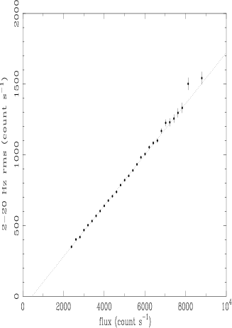
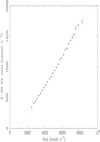
Figure 9: Comparison of rms-flux relations for real Cyg X-1 data (left) and simulated data (right) consisting of 5 independently varying light curve elements with equal mean flux and fractional rms. The grey dotted lines denote the best-fitting linear models (see text for details).

The observed lognormal flux distribution also rules out SOC models for variability, which predict a power law distribution of individual shot fluences (, 1988, 1991). The resulting distribution of the total fluxes is therefore a sum of elements with power-law distributions, with the number of summed elements depending on how much the individual shots overlap one another (, 1992). The expected flux distribution is therefore intermediate in shape between a power-law and Gaussian distribution, unlike the lognormal distribution observed here. Using a ‘shot-fitting’ approach to quantify variability, (1995) have demonstrated that the observed distribution of shot fluences in Cyg X-1 is better fitted by an exponential rather than the power-law distribution expected from SOC models. This result is probably related to the fact that the flux distribution is lognormal, and that the tail of the lognormal distribution (which is dominated by large ‘events’ which are easily picked out by shot-fitting methods) approximates an exponential distribution (see also discussion in 2002). To account for this different distribution (and also to produce more realistic PSD indices), (1995) modify the SOC model to incorporate gradual diffusion of matter through the disk. The resulting model bears some resemblance to models where the variability arises from stochastic variations in the accretion flow, rather than from the deterministic (if unpredictable) dynamics of any critical state. We also note here the temporal variability component of the ‘thundercloud model’ of (2001) which, although an additive shot-noise model, successfully produces a linear rms-flux relation. However, the thundercloud model assumes a power-law distribution of shot sizes (i.e. similar to the distribution produced by SOC models), and hence should be ruled out for the same reason as SOC models, i.e. the flux distribution is not lognormal. The reason why models with skewed (but not lognormal) flux distributions can produce linear rms-flux relations is discussed further in Appendix D.

More generally, the fact that the data are consistent with a static non-linear transform of stochastic, linear input data suggests that deterministic, non-linear types of model such as dynamical chaos are not required to explain the data. For example, a possible interpretation of apparent non-linear behaviour in light curves is that it is a result of unpredictable chaotic behaviour (the non-linearity is said to be dynamical). Such behaviour might be the signature of a rather simple physical system, which can be described by simple dynamical equations. In fact, searches for chaotic dynamics (i.e. a ‘low-dimensional attractor’) in Cyg X-1 X-ray light curves found no evidence for such behaviour (, 1989). On the other hand, possible evidence for chaotic behaviour has been suggested for the X-ray lightcurves of the microquasar GRS 1915+105 (, 2004). However, (1992) note that a succession of nested hypotheses should be tested before evidence for chaos is assumed, including whether or not the variability is consistent with static non-linearity (see also 1997). Therefore, it is possible that the static non-linear behaviour which we have demonstrated in this paper could be mistaken for dynamical chaos.

Having ruled out a large number of models, we are left wondering which models are still permitted by the data. As noted by (2003) (and see also 1988), lognormal distributions are very common in Nature, because they can be produced in a number of different ways (all involving multiplicative processes). For example, comminutive processes, involving the random splitting apart or fracturing of objects (e.g. the crushing of rocks) lead to a lognormal distribution of sizes, because the probability of a given size is dependent on a multiplicative sequence of fracture events. One could similarly envisage how multiple emitting regions following a lognormal distribution of sizes (or equivalently, fluxes) might be produced. However, it is difficult to see how such an arrangement of emitting region sizes could lead to a lognormal distribution of the total flux, unless we somehow only witness one of the emitting regions at any given time (otherwise the observed distribution would be a sum of lognormals, a possibility we have ruled out earlier in this Section). Another type of multiplicative model, involving the cumulative build up and release of energy from a reservoir, where the amount of energy released scales with total energy in the reservoir, is suggested by the jet-disc coupling model of (2004). Further investigation of these models is needed, but we note here that the lognormal form of observed data might be quite constraining for the number of components (e.g. jet, disk) which contribute (either adding or subtracting) independently to the reservoir.

Since the variability can be thought of as a static exponential transformation of linear, Gaussian data, we might first consider a direct physical interpretation of this fact. For example, the underlying variable process (e.g. variations in accretion rate) might be linear and Gaussian, but the X-ray emission process may be non-linear such that the observed X-ray variability is transformed to be non-linear and with a lognormal distribution. This possibility seems unlikely however, because (as we noted earlier), the fact that linear rms-flux relations are seen in both black hole and neutron star XRBs, which have different X-ray spectra and different emission mechanisms (e.g. 2003, 2003, 2003 and see also 2004), makes it appear unlikely that the emission process itself is the origin of the non-linearity and rms-flux relation.

An intuitive and simple way to produce the observed lognormal distribution in the underlying process is suggested by the rms-flux relation and the derivation of our exponential model which follows from it. The amplitude modulation effect implied by the rms-flux relation suggests that variations on different time-scales must multiply, rather than add, together. An obvious mechanism for coupling together variations on different time-scales is if the variations are produced at different radii in the accretion flow, with slower variations produced at larger radii. If the accretion variations can then propagate to small radii (where the X-ray emitting region exists), then variations on different time-scales can couple together, because each annulus in the accretion flow will see variations on longer time-scales produced at larger radii. Such a model was proposed by (1997), in order to explain the fact that observed X-ray variability time-scales in XRBs extend to much longer time-scales than the longest time-scales expected in the inner, X-ray emitting region (see also 2001, 2001, 2004 for enhancements to this model). (2001) then noted that the same model could explain the observed rms-flux relation - a situation that has since been reinforced by the discovery that the rms-flux relation in the X-ray millisecond pulsar SAX J1808.4-3658 is most likely produced in the accretion flow and not in a flaring corona (, 2004).

If the variations at a given radius are constant in fractional rms (e.g. as might be expected if they correspond to variations in the viscosity which are independent of mass accretion rate) then the situation is almost directly analogous to the sine multiplication picture used to derive the exponential model in this paper (here the sines represent the variations produced at different disk radii, although in reality the variations are unlikely to be periodic). Thus the rms-flux relation, lognormal flux distribution and non-linearity in the light curves can be explained in terms of a rather simple physical picture, which it should be noted can also explain the observed spectral-timing properties (energy-dependent phase lags, PSD shape and coherence) of XRBs and AGN (, 2001, 2003, 2004).

5.3 Testing future variability models

We first stress that the X-ray emission process (e.g. Comptonisation in a corona) and the fundamental origin of the variability are not necessarily implicitly related. In fact, they appear to be largely unrelated, as revealed by the fact that linear rms-flux relations are seen in both neutron star and black hole XRBs which have different X-ray emission mechanisms (, 2004). Therefore, in this Section, we will consider tests of models for the underlying variability process and not explanations of spectral variability, which are beyond the scope of this work. At the beginning of this paper, we noted that models for variability tend to start by explaining the shape of the PSD. We pointed out that the PSD is perhaps not the best tool to use to distinguish variability models, because many models can produce the required PSD shapes (e.g. using broad distributions of shot or event time-scales) and also because a standard PSD shape is in fact not a fundamental characteristic of real X-ray variability - XRBs, and possibly AGN show a variety of PSD shapes and PSD shape varies within the same state and between states. We have demonstrated in this paper three closely related characteristics of XRB and AGN variability that do have strong discriminating power between models: the rms-flux relation, non-linear variability and a lognormal distribution of fluxes. These characteristics rule out a whole swathe of models, from additive shot noise, to SOC, to any models which consist of multiple, independent varying regions whose variations add together to produce the observed variability. The variability process should be multiplicative in order to produce the observed characteristics.

Therefore, an important test of any variability model is whether it can reproduce the variability properties outlined in this paper. This fact is regardless of the specific PSD shape predicted by the model, or other properties of the variability such as spectral-timing behaviour, which can be thought of as higher-order features of any model. For example, different PSD shapes can be produced by various ‘filters’ which act on the underlying variability process (since the observed X-ray variability is only really a proxy for the underlying process). E.g. if the variability is caused by accretion rate variations, an extended distribution of the X-ray emission can act as a low-pass filter, producing a steepening of the PSD of the underlying process at high temporal frequencies along with frequency-dependent lags between different energy bands (e.g. see 2001, 2003, 2003 and 2004 for discussion). However, the observed non-linearity, rms-flux relation and flux distribution are characteristics of the underlying variability process which simple filtering cannot reproduce (since the filtering is a linear transformation of the data).

We therefore outline the following battery of tests for models of the underlying variability process. Beginning with the most important, these are:

1. . Do the model data show a linear rms-flux relation?

2. . Does the rms-flux relation occur on all time-scales, or equivalently, if the model data are stationary do the model data show a lognormal flux distribution?

3. . Does the PSD of model data match with observations?

The first two properties to be tested are likely to be most closely associated with the underlying variability process. The final test, of PSD shape, which is normally applied to variability models (e.g. 1999, 1994) is less fundamental in our opinion, because the precise PSD shape is not even a unique characteristic of variability in a single source, since PSD shape varies between states and between observations of the same state (e.g. 2003). However, the general characteristics of the PSD shape (e.g. parameterisation of the low/hard state PSD as multiple Lorentzians in both neutron star and black hole XRBs, with similar correlations between characteristic frequencies (, 2002)) are common enough to a variety of sources that the PSD shape, in combination with the first two tests, remains a useful test of the underlying variability process.

The first test, for a linear rms-flux relation, is simple to perform as an initial check of the model, but not sufficient to determine if the non-linear properties of the model are similar to those of real data. It is interesting to note here that a nearly linear rms-flux relation may be obtained from a variety of positively skewed flux distributions, if the amplitude of variability in the frequency range used to measure rms is large. We investigate the rms-flux relation for a variety of flux distributions and PSD shapes in Appendix D. However, if measured fractional rms is small (e.g. as found for the 2-20 Hz range used to measure the rms-flux relation for Cyg X-1, or the equivalent high frequencies used to measure rms-flux relations in AGN), the shape of the rms-flux relation is a strong function of the flux distribution, and in this case a linear rms-flux relation is a good predictor of an underlying lognormal distribution of fluxes. As an additional check, we then suggest carrying out the second test.

The two forms of the second test result from the fact that the lognormal flux distribution is a corollary of the fact that the rms-flux relation seems to apply on all time-scales (as is implicit in the derivation of the exponential model). If that were not the case, one would not observe a lognormal flux distribution in stationary data. However, the condition of stationarity is essential for testing for lognormality. If the simulated data are not stationary, one must instead test different time-scales of variability to see if the rms-flux relation applies (e.g. see methods in 2001, 2004 and in Section 3.2). For example, magnetohydrodynamic (MHD) simulations of turbulent accretion flows are reaching the stage where they can demonstrate the variability expected from such flows in a physically self-consistent way (e.g. 2003, 2003). However, due to current computational constraints the simulated data sets are not long enough to probe the longest variability time-scales, and hence are not stationary. Nonetheless, it would be simple to test these data sets to see if linear rms-flux relations are present on different time-scales.

Finally, we note that other tests of non-linearity, such as the bicoherence, may also impose strong constraints on models for the variability. In Section 4.3 we showed how our exponential model can explain the amplitude and general shape of the bicoherence of Cyg X-1, but not the detailed characteristics of the bicoherence. For example, the presence of apparent bumps in the bicoherence spectrum indicates stronger coupling between variations on certain time-scales than we might otherwise expect given our simple model. It is important to develop these methods of non-linear analysis to shed light on these issues, and provide further clues for the development of future models.

6 Conclusions

We have expanded on the discovery of a linear relation between rms variability and flux in XRBs and AGN, to demonstrate the following:

1. . If the linear rms-flux relation observed in XRBs and AGN applies on all time-scales, light curves $x(t)$ are produced which show a simple, formally non-linear type of variability, $x(t)=\exp[l(t)]$, where $l(t)$ is a linear input light curve.

2. . Our phenomenological, ‘exponential model’ for X-ray variability predicts a lognormal flux distribution for stationary light curves, which we confirm using data for Cyg X-1.

3. . The powerful millisecond flares observed in Cyg X-1 in the low/hard state (, 2003) are a natural consequence of the non-linear variability predicted by our model.

4. . Our model can reproduce the general shape and amplitude of the bicoherence spectrum observed in Cyg X-1 (, 2002), although detailed features in the bicoherence cannot be explained, implying a stronger coupling between certain time-scales than we naively expect from our model.

5. . Our model suggests that the clear non-linear X-ray variability observed in some NLS1 AGN results from the same variability process that applies in less variable AGN (the difference is simply that NLS1 are more variable so the non-linearity implied by our model is easier to detect). The low flux states observed in the NLS1 NGC 4051 are also a manifestation of the same variability process.

6. . Physical models for the variability must involve multiplicative processes, such as the varying-accretion model of (1997) and cannot be due to additive processes such as shot noise, or SOC processes, or multiple, independently-varying X-ray emitting regions.

7. . Future physical models for the variability should first be tested for the existence of a linear rms-flux relation. Other common tests such as PSD shape or spectral timing properties are more likely secondary characteristics of the variability process; but the rms-flux relation and the resulting non-linear variability and lognormal flux distribution (in stationary data), appear to be more fundamental features of the underlying process.

Acknowledgments

We would like to thank Tom Maccarone for useful discussions about bicoherence, and the anonymous referee for an excellent and thorough report which improved the content of this paper. PU acknowledges support from PPARC and current support from the US National Research Council. IM^cH acknowledges the support of a PPARC Senior Research Fellowship. SV acknowledges support from PPARC. This research has made use of data obtained from the High Energy Astrophysics Science Archive Research Center (HEASARC), provided by NASA’s Goddard Space Flight Center.

Appendix A A formal proof of non-linearity

We can express the exponential model for the light curve $x(t)$ in terms of the series expansion of $\exp[l(t)]$, where $l(t)$ is the linear, input light curve:

$$x(t)=\exp[l(t)]=1+l(t)+\frac{[l(t)]^{2}}{2}+\sum_{n=3}^{\infty}\frac{[l(t)]^{n}}{n!}$$ (16)

Next, we can change to discrete time steps and replace each of the $l(t)$ terms using the definition of a linear light curve in Equation 1:

$$X_{i} = 1+\sum^{\infty}_{j=0}g_{j}u_{i-j}+\frac{1}{2}\sum^{\infty}_{j=0}g_{j}u_{i-j}\left(\sum^{\infty}_{k=0}g_{k}u_{k-j}\right)$$ (17)

$$+\sum_{n=3}^{\infty}\frac{\left(\sum^{\infty}_{j=0}g_{j}u_{i-j}\right)^{n}}{n!}$$

which can be re-expressed as:

$$X_{i} = 1+\sum^{\infty}_{j=0}G_{j}u_{i-j}+\sum^{\infty}_{j=0}\sum^{\infty}_{k=0}G_{jk}u_{i-j}u_{i-k}+$$ (18)

$$\sum^{\infty}_{j=0}\sum^{\infty}_{k=0}\sum^{\infty}_{l=0}G_{jkl}u_{i-j}u_{i-k}u_{i-l}+...$$

Where the coefficients $G_{j},G_{jk},G_{jkl}\ldots\propto g_{j},g_{j}g_{k},g_{j}g_{k}g_{l}\ldots$ and the higher-order co-efficients are non-zero. Equation 18 is a Volterra series (c.f. Equation 2), an example of a formally-defined non-linear time-series model.

Appendix B The effect of the exponential transformation on PSD shape

The shape of the PSD of a linear input light curve is not preserved by the exponential transformation envisaged by our model. This can be understood in terms of the series expansion of the exponential model shown in Appendix A, where the model can be expressed in terms of the linear light curve $l(t)$ plus higher order polynomials of $l(t)$. Multiplying signals in the time domain is equivalent to convolving their Fourier transforms in the frequency domain, and the effect of convolution is to transfer power to other frequencies, thus distorting the PSD shape from its original form. Thus the effect of the exponential transformation of $l(t)$ is to add power to the PSD and transfer this power to different frequencies. It is important to take this effect into account when simulating time series using the exponential transformation, if it is necessary that the simulated light curve PSD must match some observed PSD.

Figure 10: Ratio of the PSD of simulated light curve to observed input PSD (prior to normalisation correction), for the broadband PSD shape plotted in Figure 3. See text for details.

Fortunately, for typically observed light curves, with broad continuum PSD shapes, the distorting effect of the exponential transformation is relatively small, so that it is reasonable to use the observed PSD as the PSD of the input linear light curve. In this case it is still important to apply the appropriate correction to the input PSD normalisation in order to return the correct variance in the output light curve, i.e. use Equation 14 to determine the input linear light curve variance needed to produce the required output variance and then multiply the input PSD normalisation by the ratio of the input variance to the observed variance.

As the fractional rms increases, so does the distorting effect on the PSD. However, for most observed fractional rms (e.g. 20-40 per cent) the distortion is not serious. In Fig. 10 we plot the ratio of the PSD of the simulated light curves used in Section 4 to the PSD of the observed light curve (shown in Figure 3). The variance of the simulated light curves (prior to dilution with the constant component) is $\sim 40$ per cent. The ratio is close to 1 in most cases, but increases towards high frequencies, however as the power is small at high frequencies anyway, we find this small amount of distortion acceptable.

Figure 11: Solid line: PSD (plotted as frequency$\times$power) of a simulated light curve made from an input light curve with a sharp Lorentzian PSD (shown as the dotted line).

The situation is different, and quite interesting, for input light curves with PSDs containing sharp features. In Fig. 11 we show the PSD produced by applying the exponential transformation to a light curve produced by a single sharp Lorentzian noise feature (i.e. a single QPO), with peak frequency 1 Hz, quality factor (ratio between Lorentzian frequency and full width at half-maximum) $q=10$ and a fractional rms of 50 per cent. The multiple peaks are an effect of the convolution of the PSD implicit in the exponential transformation, where the large signal at the peak of the Lorentzian couples to itself and the signals close to the peak, to produce the higher harmonics at separations of 1 Hz (in theory there should be an infinite number of such harmonics, but the 3rd harmonic is only just visible, while even higher harmonics are lost in the noise). Interestingly, a shoulder is produced at around 0.1 Hz, and in frequency$\times$power units, the flat top above the shoulder corresponds to a $1/f$ power spectral shape, with slope 0 at lower frequencies. It is interesting that the exponential transformation of a Lorentzian can produce what appears to be a rather broad continuum feature, since the correlation between sharp QPO features and break frequencies in continuum PSDs is already known in X-ray binary data (, 1999). However, we must be careful not to read too much into this interesting mathematical effect, because the simulated Lorentzian peak has a much higher normalisation than typically observed, and is still much larger than the ‘continuum’ level.

Appendix C The calculation and interpretation of bicoherence

The bicoherence $b^{2}$ is computed as follows (also see 2002 and references therein). First the light curve is split into $K$ segments, and the Fourier transform $X$ calculated for each segment. Then the bicoherence for the pair of Fourier frequencies $k$, $l$ is calculated thus:

$$b^{2}(k,l)=\frac{|\sum_{i=1}^{K}X_{i}(k)X_{i}(l)X_{i}^{\ast}(k+l)|^{2}}{\sum_{i=1}^{K}|X_{i}(k)X_{i}(l)|^{2}\>\sum_{i=1}^{K}|X_{i}(k+l)|^{2}}$$ (19)

The domain in which bicoherence measurements are independent of one another is for bifrequencies $(k,\>l)$ where $l\leq k$ and $l+k\leq N/2$ where $N$ is the number of data points in the light curve segment (i.e. $N/2$ corresponds to the Nyquist frequency). In data where the source variability is also contaminated with additive Gaussian noise, the denominator to Equation 19, which we call $A_{\rm 1}$, must be corrected for the effects of the noise (the noise cancels in the numerator to leave only the source contribution). The noise-corrected denominator $A_{\rm 2}$ can be written as:

$$A_{\rm 2} = \sum_{i=1}^{K}|X_{i}(k)X_{i}(l)|^{2}|-n^{2}(|X_{i}(k)|^{2}+|X_{i}(l)|^{2}-n^{2})$$ (20)

$$\times \sum_{i=1}^{K}\left(|X_{i}(k+l)|^{2}-n^{2}\right)$$

where $n^{2}$ is the expected noise level of the PSD due to the additive Gaussian process. The derivation of this equation is similar to that of the noise correction to the related coherence function (, 1997, 1999), which is used to examine correlations between light curve phases at identical temporal frequencies, measured in two different energy bands (unlike bicoherence which measures correlations between phases at different frequencies in the same light curve).

Since the resulting bicoherence measure is forced to lie between 0 and 1, a bias of $1/K$ must be subtracted from the bicoherence before correcting for noise, i.e. calculate bicoherence using Equation 19, then subtract $1/K$ from all measurements, and finally multiply each measurement by the ratio of denominators $A_{\rm 1}/A_{\rm 2}$. While this noise correction is effective in accounting for additive Gaussian noise, it should be noted that it is not strictly applicable for noise generated by Poisson counting statistics. The reason for this is that the amplitude of Poisson noise is correlated with $\sqrt{flux}$, so that the counting noise variations are in fact coupled to the flux variations (albeit more weakly than the intrinsic coupling between flux variations associated with the linear rms-flux relation). Therefore not only does the noise in real photon counting data affect the denominator of the bicoherence equation, it also adds to the numerator, to create a source of spurious bicoherence.

Note that the numerator of the bicoherence equation, proportional to the modulus squared of the ‘bispectrum’, averages to zero in the case of aperiodic variability with no coupling between variations on different time-scales (i.e. at different frequencies), because the phases of the signal at different Fourier frequencies are uncorrelated. In contrast, in the simple case where a pair of sine waves at frequencies $\nu_{1}$ and $\nu_{2}$ are multiplied together, the coupling of the sine waves will produce a higher frequency signal at $\nu=\nu_{1}+\nu_{2}$, which has a phase equal to the sum of phases of the two sine waves and a signal power equal to the square of the powers of the two sine waves and hence $b^{2}(\nu_{1},\nu_{2})=1$. Thus, in simple terms, the bicoherence for a given pair of frequencies $\nu_{1}$, $\nu_{2}$ indicates the fraction of the power at the frequency $\nu_{1}+\nu_{2}$ which is produced by coupling of the lower-frequency signals. It is easy to see from the series expansion of the exponential model (Appendix A) why the model will produce light curves with a significant bicoherence.

Appendix D The rms-flux relations of other distributions

In order to see how general the linear rms-flux relation is, we can consider the rms-flux relations of flux distributions other than lognormal. It is a well known result in statistics that the values of the sample variance and sample mean (i.e. estimates of mean and variance measured from a subset of an underlying population, such as a segment of a light curve) are independent if and only if the underlying population is Gaussian (e.g. 1994). However, if the distribution is not normal, e.g. it is skewed, then the sample mean and variance are not independent (with the degree of correlation scaling with the skewness of the distribution, 1985), and hence the rms from light curves with skewed distributions is correlated with flux (with the correlation having the same sign as the skewness). To determine the form of rms-flux relation resulting from different distributions, we can consider the simple case where the variance is small compared to changes in mean flux. Consider a non-Gaussian light curve $x(t)$ produced by some transformation of an underlying Gaussian light curve, $g(t)$, i.e. $x(t)=f[g(t)]$. For small changes in the flux, we can relate the variance of the Gaussian light curve $\delta g^{2}$ (which is independent of flux, and can be treated as constant in the binned rms-flux relation), to the variance of the non-Gaussian light curve $\delta x^{2}$ using the error equation (see also 1947):

$$\delta x^{2}=\left(\frac{\partial x(t)}{\partial g(t)}\right)^{2}\delta g^{2}.$$ (21)

Taking the square-root of both sides then gives an approximate expression for the rms of $x(t)$, $\sigma_{x}$. For example, in the case of a lognormal distribution, $x(t)=\exp[g(t)]$ and hence $\sigma_{x}\propto x(t)$, as expected. However, if $x(t)$ is produced by the power-law transformation of $g(t)$, $x(t)=g(t)^{\alpha}$, the relation becomes $\sigma_{x}\propto x(t)^{(1-\alpha^{-1})}$, i.e. the rms-flux relation has a power-law form. It should be stressed that this result only applies in the case where $\sigma_{x}$ is small compared to $x(t)$, i.e. the fractional rms is small. This is generally true in the case where the rms is measured at frequencies significantly above any low-frequency break in the PSD (below which PSD slope is zero), but may not be true where rms is measured close to the low-frequency break, in the regime where the data is white-noise, where the rms-flux relation can become close to linear for a wide range of skewed flux distributions. We demonstrate this effect in Fig. 12, which shows the rms-flux relations measured in the 2-20 Hz range, for simulated light curves with a distribution $x(t)=g(t)^{\alpha}$, where $\alpha=3$ and the PSD has either the same shape as seen in Cyg X-1 in Dec 1996 (Fig. 3), or is a singly broken power-law with a slope -2 above 2 Hz and slope zero below the break (hence the measured rms is a large fraction of the total rms and the mean flux).

Figure 12: Comparison of rms-flux relations for different PSD shapes and distributions $f[g(t)]$, where $g(t)$ is a Gaussian distribution of data. From top to bottom: rms-flux relation for $f[g(t)]=g(t)^{3}$ for a PSD slope of zero breaking to -2 above 2 Hz, fitted with a linear plus constant model (dotted line); $f[g(t)]=g(t)^{3}$ for a PSD similar to Cyg X-1 in 1996 Dec, fitted with a power-law of index 2/3 (dotted line); $f[g(t)]=g(t)^{2}$ for a PSD similar to Cyg X-1 in 1996 Dec, fitted with a power-law of index 1/2 (dotted line). See text for further details.

The figure shows that the data where measured rms is small follows the predicted rms-flux relation $\sigma_{x}\propto x(t)^{2/3}$, whereas the data with large measured rms shows an approximately linear rms-flux relation (including a small constant offset on the rms axis). We also show data for the Cyg X-1-like PSD corresponding to a flux distribution with index $\alpha=2$, which is well-fitted by the predicted rms-flux relation $\sigma_{x}\propto x(t)^{1/2}$. These results demonstrate that, for the kind of rms-flux relations we measure using rms at relatively high frequencies (e.g. 2-20 Hz in Cyg X-1 and equivalently high frequencies in AGN), the shape of the rms-flux relation is a good predictor of the functional form of the underlying skewed distribution. However, care must be taken when measuring large values of rms, e.g. close to the low-frequency break, since in that case, approximately linear rms-flux relations can be made for a variety of underlying distributions.

References

- (1) Aitchison J., Brown J. A. C., 1957, The Lognormal Distribution, Cambridge University Press, Cambridge
- (2) Armitage P. J., Reynolds C. S., 2003, MNRAS, 341, 1041
- (3) Bak P., Tang C., Wiesenfeld K., 1988, Phys. Rev. A, 38, 364
- (4) Bartlett M. S., 1947, Biometrics, 3, 39
- (5) Belloni T., Hasinger G., 1990, A&A, 227, L33
- (6) Belloni T., Psaltis D., van der Klis M., 2002, ApJ, 572, 392
- (7) Boller Th., Brandt W. N., Fabian A. C., Fink H. H., 1997, MNRAS, 289, 393
- (8) Box G. E. P., Cox D. R., 1964, J. R. Statistical Soc. B, 26, 211
- (9) Brandt W. N., Boller Th., Fabian A. C., Ruszkowski M., 1999, MNRAS, 303, L53 7
- (10) Christensen K., Fogedby H. C., Jensen H. J., 1991, J. Sta. Phys., 63, 653
- (11) Christensen K., Olami Z., Bak P., 1992, Phys. Rev. Lett., 68, 241
- (12) Churazov E., Gilfanov M., Revnivtsev M., 2001, MNRAS, 321, 759
- (13) Crow E. L., Shimizu K., 1988, Lognormal Distributions: Theory and Applications, Dekker, New York
- (14) Dewangan G. C., Boller Th., Singh K. P., Leighly K. M., 2002, A&A, 390, 65
- (15) Doi K., 1978, Nature, 275, 197
- (16) Done C., Gierlinski M., 2003, MNRAS, 342, 1041
- (17) Edelson R., Turner T. J., Pounds K., Vaughan S., Markowitz A., Marshall H., Dobbie P., Warwick R., 2002, ApJ, 568, 610
- (18) Fabian A. C., 1979, Proc. R. Soc. London, Ser. A, 366, 449
- (19) Fackrell J., 1996, PhD Thesis, Univ. Edinburgh
- (20) Gaskell C. M., 2004, ApJ, 612, L21
- (21) Gierlinski M., Zdziarski A. A., 2003, MNRAS, 343, L84 (GZ03)
- (22) Gilfanov M., Revnivtsev M., Molkov S., 2003, A&A, 410, 217
- (23) Gleissner T., Wilms J., Pottschmidt K., Uttley P., Nowak M. A., Staubert R., 2004, A&A, 414, 1091
- (24) Gliozzi M., Brinkmann W., Räth C., Papadakis I. E., Negoro H., Scheingraber H., 2002, A&A 391, 875
- (25) Greb U., Rusbridge M. G., 1988, Plasma Phys. & Controlled Fusion, 30, 537
- (26) Green A. R., McHardy I. M., Done C., 1999, MNRAS, 305, 309
- (27) Hinich M. J., 1982, J. of Time Series Analysis, 3, 169
- (28) Kang K., Goldsman, D., 1985, in Gantz, D., Blais, G., Solomon, S., eds, Proc. of the 17th Conference on Winter Simulation, ACM Press, New York, USA, p. 211 ESA, Noordwijk, the Netherlands, p. 499
- (29) Kantz H., Schreiber T., 1997, Nonlinear Time Series Analysis, Cambridge University Press, Cambridge
- (30) Kendall, M. G., 1994, Kendall’s Advanced Theory of Statistics 6th ed. v. 1, Edward Arnold, London
- (31) King A. R., Pringle J. E., West R. G., Livio M., 2004, MNRAS, 348, 111
- (32) Kotov O., Churazov E., Gilfanov M., 2001, MNRAS, 327, 799
- (33) Lehto H., 1989, in Hunt J., Battrick B., eds, Two Topics in X-ray Astronomy, ESA SP296. ESA, Noordwijk, the Netherlands, p. 499
- (34) Leighly K. M., 1999, ApJS, 125, 297
- (35) Leighly K. M., O’Brien P. T., 1997, ApJ, 481, L15
- (36) Lochner J. C., Swank J. H., Szymkowiak A. E., 1989, ApJ, 337, 823
- (37) Lochner J. C., Swank J. H., Szymkowiak A. E., 1991, ApJ, 376, 295
- (38) Lyubarskii Yu. E., 1997, MNRAS, 292, 679
- (39) Maccarone T. J., Coppi P. S., 2002, MNRAS, 336, 817 (MC02)
- (40) McClintock J. E., Remillard R. A., 2003, to appear in W. H. G. Lewin, M. van der Klis eds., Compact Stellar X-ray Sources, Cambridge University Press, Cambridge (astro-ph/0306213)
- (41) McHardy I. M., 1988, Mem. Soc. Astron. Ital., 59, 239
- (42) McHardy I. M., Papadakis I. E., Uttley P., Page M. J., Mason K. O., 2004, MNRAS, 348, 783
- (43) Machida M., Matsumoto R., 2003, ApJ, 585, 429
- (44) Malzac J., Merloni A., Fabian A. C., 2004, MNRAS, 351, 253
- (45) Markowitz A. et al., 2003, ApJ, 593, 96
- (46) Merloni A., Fabian A. C., 2001, MNRAS, 328, 958
- (47) Mineshige S., Ouchi N. B., Nishimori H., 1994, PASJ, 46, 97
- (48) Misra R., Harikrishnan K. P., Mukhopadhyay B., Ambika G., Kembhavi A. K., 2004, ApJ, 609, 313
- (49) Nandra K., Papadakis I. E., 2001, ApJ, 554, 710
- (50) Negoro H., Mineshige S., 2002, PASJ, 54, L69
- (51) Nowak M. A., 2000, MNRAS, 318, 361
- (52) Nowak M. A., Vaughan B. A., Wilms J., Dove J. B., Begelman M. C., 1999, ApJ, 510, 874
- (53) Pottschmidt K. et al., 2003, A&A, 407, 1039
- (54) Poutanen J., Fabian A. C., 1999, MNRAS, 306, L31
- (55) Poutanen J., Gierlinski M., 2003, MNRAS, 343, 1301
- (56) Priestley M. B., 1982, Spectral Analysis and Time Series, Academic Press, London
- (57) Quilligan F., McBreen B., Hanlon L., McBreen S., Hurley K. J., Watson D., 2002, A&A, 385, 377
- (58) Rial J. A., Anaclerio C. A., 2000, Quaternary Sci. Rev., 19, 1709
- (59) Scargle J. D., 1997, in G. J. Babu, E. D. Feigelson eds., Statistical Challenges in Modern Astronomy II, Springer-Verlag (New York), p317
- (60) Subba Rao T., Gabr M. M., 1980, J. of Time Series Analysis, 1, 145
- (61) Takeuchi M., Mineshige S., Negoro H., 1995, PASJ, 47, 617
- (62) Taylor R. D., Uttley P., McHardy I. M., 2003, MNRAS, 342, L31
- (63) Terrell N. J., 1972, ApJ, 174, L35
- (64) Theiler J., Eubank S., Longtin A., Galdrikian B., Farmer J. D., 1992, Physica D, 58, 77
- (65) Theiler J., Linsay P. S., Rubin D. M., 1994, in Weigen A. S., Gerschenfeld N. A., eds, Santa Fe Institute Studies in the Sciences of Complexity, Proc. vol. 15, Addison-Wesley, p. 429 (http://arxiv.org/abs/comp-gas/9302003)
- (66) Timmer J., König M., 1995, A&A, 300, 707
- (67) Uttley P., 2004, MNRAS, 347, L61
- (68) Uttley P., McHardy I. M., 2001, MNRAS, 323, L26
- (69) Uttley P., McHardy I. M., Papadakis I. E., Guainazzi M., Fruscione A., 1999, MNRAS, 307, L6
- (70) Uttley P., McHardy I. M., Papadakis I. E., 2002, MNRAS, 332, 231
- (71) Uttley P., Fruscione A., McHardy I. M., Lamer G., 2003, ApJ, 595, 656
- (72) Uttley P., Taylor R. D., McHardy I. M., Page M. J., Mason K. O., Lamer G., Fruscione A., 2004, MNRAS, 347, 1345
- (73) van der Klis M., 1995, in Lewin H. G., Van Paradijs J., van den Heuvel P. J., eds, X-Ray Binaries. Cambridge Univ. Press (Cambridge), p. 252
- (74) Vaughan S., Edelson R., Warwick R. S., Uttley P., 2003, MNRAS, 345, 1271
- (75) Vaughan S., Fabian A. C., Nandra K., 2003, MNRAS, 339, 1237
- (76) Vaughan B. A., Nowak M. A., 1997, ApJ, 474, L43
- (77) Wijnands R., van der Klis M., 1999, ApJ, 514, 939
- (78) Życki P. T., 2003, MNRAS, 340, 639