Coronal Electron Scattering of Hot Spot Emission Around Black Holes

Abstract

Using a Monte Carlo ray-tracing code in full general relativity, we calculate the transport of photons from a geodesic hot spot emitter through a corona of hot electrons surrounding a black hole. Each photon is followed until it is either captured by the black hole or is detected by a distant observer. The source is assumed to be a low-energy thermal emitter ($T_{\rm em}\sim 1$ keV), isotropic in the rest frame of a massive geodesic test particle. The coronal scattering has two major observable effects: the Comptonization of the photon spectrum due to the high energy electrons, and the convolution of the time-dependent light curve as each photon is effectively scattered into a different time bin. Both of these effects are clearly present in the Rossi X-Ray Timing Explorer (RXTE) observations of high frequency quasi-periodic oscillations (QPOs) seen in black hole binaries. These QPOs tend to occur when the system is in the Steep Power Law spectral state and also show no evidence for significant power at higher harmonic frequencies, consistent with the smoothing out of the light curve by multiple random time delays. We present simulated photon spectra and light curves and compare with RXTE data, allowing us to infer the properties of the corona as well as the hot spot emitter.

I INTRODUCTION

In recent years, observations of accreting black holes with the Rossi X-ray Timing Explorer (RXTE) have discovered a number of sources with high frequency quasi-periodic oscillations (HFQPOs) in their X-ray light curves. These sources are seen predominately in the Steep Power Law (SPL) spectral state, suggesting a significant level of inverse-Compton scattering of the emitted photons off of hot coronal electrons (for an excellent review of the observations, see mccli04 ).

Motivated by these observations, we extend a simple geodesic hot spot model schni04 ; schni05 to include Monte Carlo scattering of photons emitted isotropically in the hot spot’s rest frame, which then propagate through a corona surrounding the black hole. The hot spot has a planar orbit near the inner-most stable circular orbit (ISCO) and the corona is modeled with a self-similar density profile described by the advection dominated accretion flow (ADAF) model naray94 .

In Section II, we describe the physics of classical electron scattering of unpolarized light, and show how energy is transferred from high-energy electrons to low-energy photons. Section III shows how this scattering is treated in a relativistic context in the Kerr metric. Assuming a thermal emitter with $T_{\rm em}=1$ keV, we show in Section IV how the observed spectrum is modified by the hot electrons. The shape of this modified thermal spectrum can in turn be used to infer the properties of the corona.

Section V shows the time-dependent effects of scattering on the X-ray light curve, particularly how the amplitude of modulation is damped for larger optical depths. Furthermore, we find this damping is more significant for photons experiencing multiple scattering events, which tend to have higher energies. We conclude in Section VI with a summary of the implications these results have for the hot spot model for QPOs.

II ELECTRON SCATTERING

Following Rybicki & Lightman rybic79 , we use the cross section for Thomson scattering of unpolarized radiation off of nonrelativistic electrons:

$$\frac{d\sigma_{T}}{d\Omega}=\frac{r_{0}^{2}}{2}(1+\cos^{2}\theta),$$ (1)

where $r_{0}$ is the classical electron radius $r_{0}=2.82\times 10^{-13}$ cm.

It is important to note that “nonrelativistic” is a reference to the photon energy, not the electron energy. In the electron rest frame, we require $h\nu\ll m_{e}c^{2}$ in order for the above cross sections to be valid, in which case the scattering is nearly elastic or coherent. For higher energy photons, the scattering involves quantum effects and requires the “Klein-Nishina” cross section heitl54 . Since we are primarily interested in the scattering of photons from a relatively cool thermal accretion disk ($h\nu\sim 1-5$ keV), the classical treatment should suffice.

Even if the scattering is treated as coherent in the electron frame, in the lab frame energy can be (and often is) transferred from the electron to the photon. To see this boosting effect, consider a photon with initial energy $\varepsilon_{i}$ scattering off an electron with velocity $\beta$ in the $x$-direction in the “lab frame” $K$. In this frame, the angle between the incoming photon and electron velocity is $\theta$. In the electron rest frame $K^{\prime}$, the photon is scattered at an angle $\theta^{\prime}$ with respect to the $x^{\prime}$-axis. The Doppler shift formula rybic79 gives

$$\varepsilon_{i}^{\prime} = \varepsilon_{i}\gamma(1-\beta\cos\theta)$$

$$\varepsilon_{f} = \varepsilon_{f}^{\prime}\gamma(1+\beta\cos\theta^{\prime}),$$ (2)

where $\gamma=1/\sqrt{1-\beta^{2}}$ and $\varepsilon_{f}$ is the post-scattering energy in the lab frame. In the electron frame, we assume elastic scattering with $\varepsilon_{i}^{\prime}=\varepsilon_{f}^{\prime}$, which should be the case for the typical seed photons from a thermal emitter at $T_{\rm em}\sim 1$ keV.

Averaging over all angles $\theta$ (isotropic electron distribution) and $\theta^{\prime}$ [weighted by eqn. (1)], we find that the typical scattering event boosts the photon energy by

$$\frac{\varepsilon_{f}}{\varepsilon_{i}}\approx\gamma^{2}.$$ (3)

To determine $\gamma$, we consider a Maxwell-Boltzmann distribution function in electron momentum $p=\gamma mv$:

$$f(p)d^{3}\mathbf{p}\propto 4\pi p^{2}\exp\left(-\frac{\sqrt{p^{2}c^{2}+m_{e}^{2}c^{4}}}{kT_{e}}\right).$$ (4)

III RELATIVISTIC IMPLEMENTATION

Unlike the approach taken in schni04 , where the photons were traced backwards in time from a distant observer to the emitting region, here it is conceptually easier to trace the photons forward in time from the emitter to the observer, then use Monte Carlo methods to determine the distribution of scattered photons. For the Thomson cross section, the path of each photon is energy-independent, so the photon’s final observed energy can be thought of as a fiducial redshift $E_{\rm obs}/E_{\rm em}$ that can be convolved with the spectrum in the local emitter frame to produce the total spectrum seen by the observer.

To determine the initial momentum of each photon, we construct a tetrad centered on the emitter’s rest frame, denoted by tilde indices $\tilde{\mu}$. In the coordinate basis, the energy and angular momentum of a particle on a stable circular orbit around a Kerr black hole are given by

$$-p_{t}({\rm em})=\frac{r^{2}-2Mr\pm a\sqrt{Mr}}{r(r^{2}-3Mr\pm 2a\sqrt{Mr})^{1/2}}$$ (5)

and

$$p_{\phi}({\rm em})=\pm\frac{\sqrt{Mr}(r^{2}\mp 2a\sqrt{Mr}+a^{2})}{r(r^{2}-3Mr\pm 2a\sqrt{Mr})^{1/2}}.$$ (6)

From these we construct the 4-velocity via the inverse metric $p^{\mu}({\rm em})=g^{\mu\nu}p_{\nu}({\rm em})$, which gives $\mathbf{e}_{\tilde{t}}$. Then $\mathbf{e}_{\tilde{r}}$ and $\mathbf{e}_{\tilde{\theta}}$ are defined parallel to the coordinate basis vectors $\mathbf{e}_{r}$ and $\mathbf{e}_{\theta}$, and $\mathbf{e}_{\tilde{\phi}}$ is given by orthogonality.

In this basis, the initial photon direction is picked randomly from an isotropic distribution, uniform in spherical coordinates $\cos\tilde{\theta}=[-1,1]$ and $\tilde{\phi}=[0,2\pi)$. All photons are given the same initial energy in the emitter frame $p_{\tilde{t}}=-E_{0}$, which is used as a reference energy for calculating the final redshift with respect to a stationary observer at infinity. Given $p_{\mu}$, the photon’s geodesic trajectory is integrated using the Hamiltonian formulation described in schni04 .

Figure 1: Planar photons emitted isotropically in the rest frame of a massive particle on a circular orbit at the ISCO. The photon paths are colored according to their red- or blue-shift in energy with respect to $E_{0}$ measured in the emitter’s frame.

Figure 1 shows an “overhead view” of photon trajectories in the plane of the disk, emitted isotropically by a massive test particle on a circular orbit at the ISCO of a black hole with $a/M=0.5$. The photons are colored according to their energy-at-infinity $E_{\rm obs}=E_{\infty}=-p_{t}$, either blue- or redshifted with respect to their energy in the emitter frame $E_{0}$. The relativistic beaming is done automatically by the Lorentz boost from the emitter to the coordinate frame, so the blue photons are clearly bunched more tightly together, as required by the invariance of $I_{\nu}/\nu^{3}$.

At each step along the photon’s path, we determine the probability of electron scattering according to the differential optical depth $d\tau_{\rm es}=\kappa_{\rm es}\rho ds.$ The density $\rho$ is defined in the “Zero Angular Momentum Observer” (ZAMO) frame barde72 and the opacity $\kappa_{\rm es}$ is given by the classical cross section quoted above in equation (1). The scattering is then treated classically in the electron’s local frame, after which the new photon 4-momentum is transformed back to the coordinate basis and the ray-tracing continues along the new trajectory.

IV EFFECT ON SPECTRA

As we showed at the end of the Section II, one effect of the coronal scattering is generally a transfer of energy from the electron to the photon. One way to quantify this energy transfer is through the Compton $y$ parameter, defined as the average fractional energy change per scattering, times the number of scatterings through a finite medium. For nonrelativistic electrons, Rybicki & Lightman rybic79 show that the average energy transfer per scattering event is

$$\frac{\varepsilon_{f}-\varepsilon_{i}}{\varepsilon_{i}}=\frac{4kT_{e}}{m_{e}c^{2}}.$$ (7)

The mean number of scatterings for an optically thin medium is simply $\tau_{\rm es}$, the total optical depth through the medium. For optically thick systems, the photons must take a random walk to escape, so the number of scatterings becomes $\tau^{2}_{\rm es}$. Thus the Compton $y$ parameter for a finite medium of nonrelativistic electrons is

$$y=\frac{4kT_{e}}{m_{e}c^{2}}\mbox{Max}(\tau_{\rm es},\tau_{\rm es}^{2}).$$ (8)

For a low-energy soft photon source with multiple scattering events, the final spectrum due to inverse-Compton scattering can be estimated using the Kompaneets equation. For $kT_{\rm em}\lesssim h\nu\lesssim kT_{e}$, the resulting spectrum takes the power-law form

$$I_{\nu}\sim\nu^{-\alpha},$$ (9)

with

$$\alpha=\frac{3}{2}+\sqrt{\frac{9}{4}+\frac{4}{y}}.$$ (10)

At energies above $kT_{e}$, the electrons no longer efficiently transfer energy to the photons, so the spectrum shows a cutoff for $h\nu\gtrsim kT_{e}$:

$$I_{\nu}\sim\nu^{3}\exp(-h\nu/kT_{e}).$$ (11)

With the assumption of purely elastic scattering, we cannot actually reproduce this cutoff effect; all photons are scattered equally, and the ratio $\varepsilon_{f}/\varepsilon_{i}$ is independent of energy. Thus equation (7) would predict infinite energy boosts until $h\nu\gg m_{e}c^{2}$. In reality, higher energy photons tend to lose energy in scattering, due to the recoil of the electron. This effect is relatively easy to calculate from conservation of energy and momentum in the electron rest frame:

$$\varepsilon_{f}=\frac{\varepsilon_{i}}{1+\frac{\varepsilon_{i}}{m_{e}c^{2}}(1-\cos\theta)}$$ (12)

To accurately include this effect, we would have to keep track of the real “physical” energy of each photon, instead of the fiducial redshift method that we currently use to reconstruct the total spectrum afterwards. Ultimately, this is just a matter of computational intensity and no real conceptual difficulty. To first-order, we can treat the thermal photon source as a monochromatic emitter at $E_{0}=3kT_{\rm em}$, which gives a reasonable approximation to the true solution.

For the corona geometry, we use a self-similar distribution described by an ADAF model naray94 , with density and temperature profiles that scale as

$$\rho \propto r^{-3/2},$$ (13)

$$T \propto r^{-1}$$ (14)

outside of the ISCO. We have ignored the bulk velocity of the inwardly flowing gas, which will typically have $v_{\rm bulk}\ll v_{\rm therm}$ in the ADAF model.

Without scattering, the time-averaged “numerical” spectrum could be described by the relativistic transfer function described in schni04 , defined over an infinitesimal band in radius $R_{\rm in}\approx R_{\rm out}=r_{\rm em}$. The inverse-Compton processes in the corona serve to further broaden this transfer function, as in sunya80 and titar94 . This transfer function is then normalized to the rest energy $E_{0}$ and convolved with the actual emission spectrum (e.g. a thermal blackbody at $kT_{\rm em}$) to give the simulated observed spectrum.

Figure 2: Simulated observed spectra of a thermal hot spot emitter with $T_{\rm em}=1$ keV, on a circular orbit at the ISCO of a black hole with $a/M=0.5$. The thermal spectrum is modified by relativistic effects and Compton scattering off a hot corona with $T_{e}=(r_{\rm ISCO}/r)100$ keV.

Figure 2 shows a set of these simulated spectra from a hot spot emitter around a black hole with $a/M=0.5$. The emission spectrum is thermal in the hot spot rest frame with $T_{\rm em}=1$ keV. The coronal ADAF model has $T_{e}=(r_{\rm ISCO}/r)100$ keV, and electron density $n_{e}\sim r^{-3/2}$ for a variety of optical depths $\tau_{\rm es}$. The spectra are plotted in units of (#photons/s/cm²/keV), as is the convention by many observers, but the actual magnitude of the $y$-axis is arbitrary, and would normally depend on the distance to the source. From the slope of the power-law and the location of the cut-off, the corona temperature and optical depth can be inferred from observations pozdn77 ; sunya79 ; gilfa94 ; gierl97 .

V EFFECT ON LIGHT CURVES

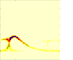
Figure 3: Time-dependent spectra of a monochromatic, isotropic hot spot emitter on an ISCO orbit with $a/M=0.5$ and inclination angle $i=75^{\circ}$. The four panels show spectrograms for systems of increasing optical depth $\tau_{\rm es}=[0,1,2,4]$. The logarithmic color scale shows the number of photons in each time/energy bin, normalized to the peak value for each panel.

The spectra in Figure 2 were created by integrating over the complete hot spot orbital period and over all observer inclination angles. However, during the Monte Carlo calculation, it is just as simple to bin all the photons according to their final values of $\theta$, $t_{\rm obs}$, and energy $-p_{t}$. The latitude bins are evenly spaced in $\cos\theta$ so that a comparable number of photons land in each zone. The energy bins are spaced logarithmically to include the high energy tail and also maintain high enough spectral resolution at lower energies. Assuming the hot spot is on a circular periodic orbit, the photons detected at any azimuthal position can be mapped into the appropriate bin in $t_{\rm obs}$, so that none are “wasted.”

An excellent way to see the effects of scattering on the hot spot light curves is by plotting time-dependent spectra of a monochromatic emitter, shown in Figure 3 for a range of optical depths and an inclination angle of $75^{\circ}$. The logarithmic color scale shows (#photons/s/cm²/keV/period), normalized to the peak intensity in each panel. At “0” phase, when the emitter is on the far side of the black hole, the spectrum shows two distinct lines, one blueshifted in the forward direction of hot spot motion, and one redshifted in the backward direction. As the hot spot comes around towards the observer, the directly beamed blueshifted line dominates, and then when the phase is $\sim 0.5$ and the hot spot is on the near side of the black hole, a single line dominates. This is due to the gravitational demagnification of the secondary images formed by photons that have to complete a full circle around the black hole to reach the observer. While these features would most likely be unresolvable for black hole binaries, they may well be observable in X-ray flares from Sgr A^∗ as well as other supermassive black holes (e.g. see bagan01 ).

In the subsequent panels, the spectrum is modified by the scattering of the hot spot photons in the surrounding corona. As in Section IV, the temperature and density profile of the corona is given by an ADAF model with $T_{e}(r_{\rm ISCO})=100$ keV. The four panels of Figure 3 show increasing values of $\tau_{\rm es}=[0,1,2,4]$. The effects of scattering on the spectra are really quite profound. As we described qualitatively in schni05 , the electron corona is like a cloud of fog surrounding a lighthouse, spreading out the delta-function beam in time and energy.

Unlike the simple model there, where each photon was assigned some positive time delay, the full Monte Carlo scattering calculation shows that some photons actually arrive earlier in time by taking a “shortcut” to the observer instead of waiting for the hot spot to come around and move towards the observer. And of course, the photons are also spread out in energy due to the inverse-Compton effects. As the optical depth increases, the well-defined curves in Figure 3a is smeared out into a nearly constant blur when $\tau_{\rm es}=4$, with a broad spectral peak as in Figure 2. Only a slight trace of the original coherent light curve remains, composed of roughly $1\%$ of the emitted photons that do not scatter before reaching the observer or get captured by the event horizon. When $\tau_{\rm es}>1$, multiple scattering become more common, so photon shortcuts become rarer, tending to spread the light curve preferentially to the right (delay in observer time), as seen in Figures 3c,d.

By integrating over broad energy bands such as those typically used in RXTE observations, we can increase our “signal” strength while sacrificing spectral resolution. For millisecond periods, there will still not be nearly enough photons to provide phase resolution, but these features may show up statistically in the power spectrum or bispectrum macca04 . Figure 4 shows a set of integrated light curves for a variety of optical depths. The black hole and hot spot parameters are as in Figure 3, here assuming a thermal hot spot emitter with temperature $T_{\rm hs}=1$ keV. As the optical depth to electron scattering increases, the rms amplitude of each light curve decreases as the photons get smoothed out in time. Similarly, due to the average time delay added to each photon by the increased path length, the relative location of each peak is shifted later in time.

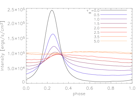
Figure 4: Energy-integrated light curves for a hot spot with orbital parameters as in Figure 3 and a range of coronal optical depths. The emitted spectrum is assumed to be thermal with a hot spot temperature $T_{\rm hs}=1$ keV, integrated over $0.5-30$ keV in the observer’s frame.

In all likelihood, the relative phase shifts would be nearly impossible to detect, regardless of the instrument sensitivity, since to do so would require measuring the light curve from a single coherent hot spot at two different optical depths. It is difficult to imagine a scenario where the coronal properties could change on such short time scales (yet it is possible that a fixed hot spot on the surface of an X-ray pulsar might actually be used for this technique). However, the higher harmonic peaks of the different light curves may in fact be measurable with the next-generation X-ray timing mission, or under extremely favorable conditions, even with RXTE.

While the absolute peak shifts for hot spot light curves at different optical depths would probably not be detectable, the relative shifts of simultaneous light curves in different energy bands may be observable, at least on a statistical level with a cross-correlation analysis. Since the average scattering event boosts photons to higher energy bands and also causes a net time delay due to the added geometric path, the light curves in higher energy bands should be delayed with respect to the lower energy light curves. A few of the typical energy bands used for RXTE observations are $(2-6)$, $(6-15)$, and $(15-30)$ keV. To fully cover the peak emission from a thermal hot spot at 1 keV, we expand the lowest energy band in our calculations to cover $(0.5-6)$ keV. The light curves in these three bands are plotted in Figure 5 for $i=75^{\circ}$. The low energy band resembles the unscattered light curve plus a roughly flat background, while the higher energy light curves show a much smaller modulation with a significant phase shift ($\sim 0.3$ periods) due to the additional photon path lengths.

Figure 5: Hot spot light curves in a few different RXTE energy bands (we have expanded the lowest energy band down to 0.5 keV to include the thermal emission of a hot spot at $T_{\rm hs}=1$ keV). The hot spot inclination is $75^{\circ}$ and the coronal properties are as in Figure 3. The optical depth to scattering is $\tau_{\rm es}=1.5$ in (a) and $2.5$ in (b). The higher energy light curves are made from photons that have experienced more scattering events, boosting their energy and delaying their arrival time.

VI IMPLICATIONS FOR QPO MODELS

The original motivation for the application of scattering to the hot spot model was to answer a few important questions raised by RXTE observations:

• The distinct lack of power in higher harmonics at integer multiples of the peak frequencies.

• The larger significance of high frequency QPO detections in the higher energy bands (6-30 keV) relative to the signal in the lower energy band (2-6 keV).

• The trend for these HFQPOs to exist predominantly in the Steep Power Law (SPL) spectral state of the black hole.

Beginning with the final point, it appears to be quite reasonable that the physical mechanism producing the power law region of the spectrum is the inverse-Compton scattering of cool, thermal photons off of hot coronal electrons. The steep power law suggests a small-to-moderate value for the Compton $y$ parameter, inferred from equation (10), in the range $0.5\lesssim y\lesssim 10$. From equation (8), this suggests either a small optical depth or a small electron temperature. To gain insight into which of these two options is more likely, we need to address the other two observational clues.

In schni05 , we first proposed the scattering model as an explanation for harmonic damping. With the more careful treatment in this paper, we include not only the temporal, but also the spatial effects of electron scattering. The photons originally beamed toward the observer are now scattered in the opposite direction, while the photons emitted away from the observer can now be scattered back to him. This smoothes out the light curve in time more effectively than the localized convolution functions used in schni05 . At the same time, the scattering is not completely isotropic [see eqn. (1)], so some modulation remains. Thus, to maintain a significant modulation in the observed light curve, we require a relatively small optical depth, reducing the smoothing effects of the scattering.

The fact that most HFQPOs appear more significantly in higher energy bands also points towards Compton scattering off hot electrons. However, as the calculations above show (see Fig. 5), with the basic thermal disk/hot spot model, the light curves actually have smaller amplitude fluctuations in the higher energy bands, as these scattered photons get smoothed out more in time. Furthermore, while the higher harmonic modes are successfully damped in the scattering geometry, so is the fundamental peak. Thus, in order to agree with observations, the hot spot overbrightness would need to be much higher than the values quoted in schni04 ; schni05 .

Based on these arguments alone, we find it unlikely that the HFQPOs are coming from a cool, thermal hot spot getting upscattered by a hot corona. From the photon continuum spectra of the SPL state, there appears to be a hot corona with $T_{e}\sim 100$ keV, but as Figure 5a shows, the lowest energy photons, which presumably do not scatter in the corona, have by far the greatest amplitude modulations. It is possible that the relative modulation would appear smaller due to the added flux from the rest of the cool, thermal disk, but much of this steady-state emission should also get scattered to higher energies, further damping the modulations in the $(6-30)$ keV bands.

The high luminosity of the SPL state (also called the Very High state) suggests that the thermal, slim disk geometry may not be appropriate here. Perhaps it is more likely that these cases correspond to an ADAF model, traditionally associated with very low or very high accretion rates naray94 . Since the ADAF model cannot radiate energy efficiently, the gas in the innermost regions will be much hotter than in the slim disk paradigm. Thus hot hot spots with $T_{\rm hs}\gtrsim 5$ keV could be forming inside a small ADAF coronal region, providing seed photons that are already in the higher energy bands, and are only moderately upscattered by the surrounding corona.

Future work will focus on exploring other corona geometries and applying the Monte Carlo scattering code to other QPO models in order to better understand the emission processes that describe the SPL spectral state.

- (1) F.K. Baganoff, et al., Nature 413, 45 (2001).
- (2) J.M. Bardeen, W.H. Press, & S.A. Teukolsky, ApJ 178, 347 (1972).
- (3) M. Gierlinsky, et al., MNRAS 288, 958 (1997).
- (4) M. Gilfanov, et al., ApJS 92, 411 (1994).
- (5) W. Heitler, The Quantum Theory of Radiation, (London: Oxford University Press) (1954).
- (6) T.J. Maccarone & J.D. Schnittman, MNRAS in press, preprint (astro-ph/0411266) (2005).
- (7) J.E. McClintock & R.A. Remillard, R. A., in Compact X-ray Sources, ed. W. H. G. Lewin & M. van del Klis (New York: Cambridge Univ. Press), preprint (astro-ph/0306213) (2004).
- (8) R. Narayan & I. Yi, ApJ 428, L13 (1994).
- (9) L.A. Pozdniakov, I.M. Sobol, & R.A. Sunyaev, Sov. Astron. 21, 708 (1977).
- (10) G.B. Rybicki & A.P. Lightman, Radiative Processes in Astrophysics, (New York: Wiley-Interscience) (1979).
- (11) J.D. Schnittman & E. Bertschinger, ApJ 606, 1098 (2004).
- (12) J.D. Schnittman, ApJ in press, preprint (astro-ph/0407179) (2005).
- (13) R.A. Sunyaev & J. Truemper, Nature 279, 506 (1979).
- (14) R.A. Sunyaev & L.G. Titarchuk, A&A 86, 121 (1980).
- (15) L.G. Titarchuk, ApJ 434, 570 (1994).