Contributed paper at the conference VAK-2004 ”Horizons of Universe”

held in Moscow, Russia June 3 - 10, 2004

We present a technique for the successive restoration of the branches of the one-dimensional strip brightness distribution across a quasar’s accretion disk via the analysis of observations of high magnification events in measured fluxes from the multiple quasar images produced by a gravitational lens. Hypothesizing these events to by associated with microlensing by a fold caustic, the branches of brightness distribution are searched for on compact sets of non-negative, monotonically non-increasing, convex downward functions. The results of numerical simulations show that the solution obtained is stable against random noise. Analysis of the light curves of high magnification events in the fluxes from components C and A of the gravitational lens QSO 2237+0305, observed by the OGLE and GLITP groups, has yielded the forms of the strip brightness distributions across the accretion disk of the lensed quasar. The resulting sizes of the accretion disk are in agreement with results obtained earlier via model-fitting. The form of the brightness distribution is consistent with the expected appearance of an accretion disk rotating around supermassive black hole.

1. Introduction

According to our current understanding, the main source of the energy of quasars and other active galactic nuclei (AGN) is the accretion onto a supermassive black hole. The properties of the accretion disk that is formed determine to an appreciable extent the observed characteristics of these objects [1]. One way to study accretion processes is via spectral analyses, including investigations of the X-ray lines profiles and the reverberation mapping or echo tomography of the disks [2]. Such studies have yielded most of the currently available information.

Another independent way to obtain information about the accretion processes is to investigate the spatial structure of the disk, which requires observations with very high angular resolution, exceeding a microsecond of arc. In spite of the seemingly unrealistic smallness of this value, a proposed space X-ray interferometer project [3] would, in fact, provide this resolution. However, a similar resolution can be obtained in the visible using observations of gravitational lens systems: intervening galaxies that give rise to multiple images of distant quasars. Microlesing by stars in the lens galaxy produces a random field of caustics, which can lead to a high magnification event (HME) in the measured fluxes from the images when a caustic crosses the accretion disk of the quasar [4,5]. The most probable type of microlensing occurs when a fold caustic intersects the disk, in which case the observed light curve contains information about the one-dimensional strip brightness distribution across the accretion disk in the direction of the local normal to the caustic. Restoration of this strip distribution from observational data involves solution an ill-posed inverse problem, and requires the use of special algorithms that are stable against random noise. This problem was first considered by Griegar et al. [6], who used the Tikhonov’s regularization method.

The more interesting problem of restoration of the radial brightness distribution in the locally co-moving frame of the accretion disk was first analyzed by Agol and Krolik [7], who also used the Tikhonov’s regularization method. This problem is significantly more difficult, and requires, in addition to the introduction of a number of free parameters to describe the microlensing geometry, the consideration of relativistic effects. For observations obtained in a single photometric band, it is not possible to take relativistic effects into account without a disk model that describes how the radiation intensity of a disk area element depends on direction and frequency. The attempt of Mineshige and Yonehara [8] to restore the radial brightness distribution in the accretion disk seen by an external distant observer was not successful in this sense, since their solution assumed circular symmetry, which will not be the case in the presence of relativistic effects. In spite of the possibility of deriving the radial brightness distribution in an accretion disk in a locally co-moving frame, the restoration of the strip brightness distribution in a frame of a distant observer remains an important problem. This is true because the form of the strip brightness distribution can be restored using minimum a priori information without knowledge of the caustic parameters, distances to the source and lens, or the relative velocity of the source and lens. There is no need to introduce any model constraints on the properties of the lensed source.

The gravitational lens QSO 2237+0305, which is also called Huchra’s lens or the Einstein cross, is the best know representative of this class of objects. Four images of a distant ($z_{s}=1.695$) quasar are created by the gravitational field of a fairly nearby ($z_{d}=0.0394$) galaxy that is lying nearby in the line of sight to the observer. As a result, the time delay between the light variations for different images is less than a day, and the characteristic duration of the HMEs should be several tens of days. Uncorrelated fluctuations in the fluxes from the different images that were probably associated with microlensing by stars in the lens galaxy were first detected by Irwin et al. [9] and used to estimate the size of the accretion disk [10,11]. Later, various groups of observers monitored this object in hopes of detecting the effects of microlinsing [12-15].

The most complete series of observations, obtained by the international OGLE group [16,17], demonstrated the presence of possible HMEs in components A (in 1998) and C (in Summer 1999). The observational data for these events were analyzed with the aim of deriving the size of the accretion disk, both using statistical methods [18,19] and via model-fitting of the brightness distribution for a circularly symmetric source [20,21].

Alcalde et al. [22] recently presented observations by the GLITP group that nicely supplement the data of the OGLE group in Autumn 1999; these display the HME in component A. Based on the hypothesis that this event was associated with microlensing by a fold caustic, these observations were analyzed by fitting both symmetric source models [23] and a model brightness distribution of the form expected for a standard geometrically thin and optically thick Newtonian accretion disk [24] surrounding a Schwarzschild black hole, allowing for the inclination of the plane of the disk to the line of sight [25]. In the latter case, it was possible to derive constraints on the mass of the black hole at the center of the quasar:$\ 10^{7}M_{\odot}<M<6{\times}10^{8}M_{\odot}$.

Together with many advantages, the model-fitting also has certain disadvantages. The main one is the possibility that model is inadequate to the real object. It is clear, for example, that the possibility that plane of the disk is inclined to the line of sight makes circularly symmetrical models potentially inadequate. Similarly, there is a good basis to suppose that there should be a Kerr black hole rotating at close to the maximal rotation rate at the center of a quasar [1]. In this case, the accretion disk is appreciable relativistic. The edge of the rotating disk that is approaching the observer will appear to be brighter than the receding edge, leading to a loss of symmetry in both radial brightness distribution and strip brightness distribution across the disk. Therefore, model-independent methods for the analyses of observational data based on the restoration of the brightness distribution are especially important.

The important censorious remark must be made relative to the use of the Tikhonov’s regularization method. Unlike the binary-lens case, in which caustics are isolated and their crossing by a source can be clearly fixed, microlensing by stars of a lens galaxy produces a random field of caustics in the source plane. The neighboring caustics also contribute to observed flux variations. Their influence can be minimized by analyzing only part of the light curve near its maximum. In this case, however, it becomes impossible to determine the initial flux level, relative to which the flux varies as additional images appear or disappear during the primary caustic crossing that led to the HME. This initial flux level cannot be derived directly from the light curve.

At first glance, it seems that this problem has a simple solutions - allowing the initial level to be a free parameter and estimating it by requiring the best fit to the observational data. However, this approach automatically makes it impossible to apply the Tikhonov’s regularization method used in [6-8] to restoration of the brightness distributions. It is known that the approximate solution of the ill-posed inverse problem yielded by this method is the smoothest function whose lensing curve agrees with the observational data within the errors [26,27]. Varying the initial level produces a family of strip brightness distribution. All functions of this family, including those having no physical meaning, will give the same goodness-of-fit to the observations. There is no criterion that can be used to select one of these function as the best approximate solution. In addition, the Tikhonov’s regularization method makes the minimum use of a priori information about the solution of the ill-posed problem, and is therefore not able to provide good stability of the solution at large noise level.

The purpose of our paper is the description of the new technique of the analysis of observational data by invoking additional a priori information consistent with the physics of the phenomenon, and results of its application to the analysis of the HMEs observations in components of the gravitational lens QSO 2237+0305. These results were published partially in the papers [28,29].

2. Method for restoration of strip brightness distribution across source

Let us suppose that the image of a quasar’s accretion disk is scanned by a fold caustic, which can be taken to have the form of a straight line due to the small angular size of the disk. Let $b(x,y)$ be the brightness distribution in the disk for a distant external observer in a Cartesian coordinate system $(x,y)$ in the plane of the sky, with the $x$ axis oriented perpendicular to the caustic and the coordinate origin coincident with the center of the disk. The observed lensing curve will then depend only on the one-dimensional strip brightness distribution $B(x)$, defined by expression

$$B(x)=\int_{-\infty}^{\infty}\int_{-\infty}^{\infty}b(\xi,y)\delta(\xi-x)\,d\xi dy,$$

where $\delta(x)$ is the Dirac delta function. When the caustic crossing leads to the appearance of additional images of the source accompanied by a sharp amplification of the flux, the HME light curve $I(x)$ is given by the convolution integral equation

$$I(x)=A(x)*B(x)=\int_{-\infty}^{\infty}A(x-\xi)B(\xi)\,d\xi,$$

whose kernel has the form [30-32]

$$A(x-\xi)=A_{0}+\frac{K}{\sqrt{x-\xi}}H(x-\xi),$$

where $H(x-\xi)$ is the Heavyside step function, which is equal to zero for negative and unity for non-negative values of its argument. The quantity $A_{0}$ in (3) depends on the initial flux level, which is produced by all the other images of the source and remains unchanged during the caustic crossing, and the factor $K$ characterizes the amplification of the caustic. The values of $A_{0}$ and $K$ are usually not known. When (3) is substituted into (2), we can see that $A_{0}$ determines the initial flux level $I_{0}$ , which as we said in the introduction, is a free parameter of the inverse problem. The absence of information about $K$ means that $B(x)$ can be restored only up to a constant factor. The second free parameter is the time when the caustic passes through the center of the disk $t_{0}$ , which determines the origin for the $x$ axis. If the projection of the tangential velocity of the caustic onto this axis is $V_{\perp}$, the time dependence of the spatial variable $x$ has the form $x=V_{\perp}(t-t_{0})$. As for the parameter $K$ from (3), the scanning velocity $V_{\perp}$ is, in general, unknown. Setting $K=1$ and $V_{\perp}=1$ and assuming $x=t-t_{0}$ , we can restore only the form of the strip brightness distribution $B(x)$ from observations of the HME.

Since the quasar accretion disk is appreciably relativistic, if the rotational axis is inclined to the line of sight, the brightness of an area element approaching the external observer should exceed the brightness of a receding area element [7]. Therefore, apart from cases where the caustic scan is directed along the rotational axis, $B(x)$ ceases to by an even function. We can now write the initial integral in (2) as a sum of two integrals taken along negative and non-negative intervals. Performing a substitution of variables in the first of these integrals, we obtain

$$I(x)=\int_{0}^{\infty}A(x+\xi)B(-\xi)\,d\xi+\int_{0}^{\infty}A(x-\xi)B(\xi)\,d\xi.$$

It can easily be seen that the properties of the kernel (3) imply that for $x\in(-\infty,0]$ the second integral in (4) vanishes. It follows that only the negative branch of the strip brightness distribution contributes to the formation of the negative branch of the lensing curve, whereas both branches affect the positive branch $I(x)$ when $x\in(0,\infty)$.

The analysis of the strip brightness distributions for relativistic accretion disks [28] shows that for optical and IR radiation outside the small region $\mid\xi\mid\leq\xi_{0}$, which makes a negligibly small contribution to the total flux, $B(-\xi)$ for $\xi\in(-\infty,-\xi_{0}]$ and $B(\xi)$ for $\xi\in[\xi_{0},\infty)$ are either non-negative, monotonically non-increasing or non-negative, monotonically non-increasing, convex downward functions. It is known that the sets of functions of these types are the compact sets. The search for the solution of an ill-posed problem on the compact set of functions gives the unique and stable result [26,27]. Thus, we can regard the branches of $B(\xi)$ as members of the compact set of these functions. This a priori information is qualitative and imposes no rigid model constraints on the form of the strip brightness distribution.

The values of free parameters $I_{0}$ and $t_{0}$ can be determined from the minimum residual corresponding to the restored function $B(x)$, which is usually found using the sum of the squared deviations, or the quantity $\chi^{2}_{N}$ . Since the set of functions on which the search for the solution is carried out is compact, this guarantees that the obtained profiles $B(x)$ and the values of the free parameters will approach their exact values as the errors in the estimate of the observed flux $I(x)$ approach zero [26,27]. The use of a large amount of a priori information about the possible form of the strip brightness distribution in accordance with the physics of phenomenon enables us to achieve a solution with a high degree of stability against the effects of random noise.

Given the above considerations, we have formulated the following algorithm for successive restoration of the branches of the strip brightness distribution assuming $K=1$,$\ V_{\perp}=1$ and $x=t-t_{0}$ .

Step 1. Specify the initial values of the free parameters $I_{0}$ and $t_{0}$ .

Step 2. On the negative branch of the lensing curve $I(x)$ for $x\in(-\infty,0]$, solve the inverse problem for the integral equation

$$I(x)=\int_{0}^{\infty}A(x+\xi)B(-\xi)\,d\xi$$

and find the negative branch $B(-\xi)$ for $\xi\in(-\infty,-\xi_{0}]$ on one of the compact sets of functions.

Step 3. Modify the positive branch of the lensing curve for $x\in(0,\infty)$ as follows:

$$\tilde{I}(x)=I(x)-\int_{0}^{\infty}A(x+\xi)B(-\xi)\,d\xi.$$

Step 4. Solve the inverse problem for the integral equation

$$\tilde{I}(x)=\int_{0}^{\infty}A(x-\xi)B(\xi)\,d\xi$$

for $x\in(0,\infty)$ and find the positive branch of $B(\xi)$ for $\xi\in[\xi_{0},\infty)$ on the same compact set of functions.

Step 5. Compute the value of the total residual function for both branches of the lensing curve.

Repeating the steps 1 - 5, we can easily find the global minimum of the residual function by exhausting all possible free parameter combinations. The values of parameters $I_{0}$ and $t_{0}$ and the two branches of the strip brightness distribution corresponding to this minimum yield the optimal approximate solution of the problem.

A similar technique for the successive restoration of the branches of $B(\xi)$ can be used when a caustic crossing involves the disappearance of source images, resulting in an abrupt flux decrease. In this case, the argument of the kernel (3) has the opposite sign. Therefore, only the positive branch of $B(\xi)$ contributes to positive branch $I(x)$, whereas both branches of the strip brightness distribution contribute to the formation of the negative branch $I(x)$.

We should note one other important circumstance, which has usually been neglected in the studies of the HMEs cited above. The main integral equation (2) has the singular kernel (3). When calculating such integrals, it is necessary to take special measures to ensure convergence of the corresponding integral sums. In particular, attempts to calculate the values $I(x_{i})$ on non-uniform grid $x_{i}$ when $B(\xi_{i})$ is specified on a uniform grid can lead to large errors in the results. General questions with regard to the application of numerical methods for singular integral equations are considered in [33]. A simple proof of a sufficient condition for the convergence of the integral sums for the specific case of (2) with the kernel (3) is presented in [34]. This condition consist of the special selection of grids forming a so-called canonical dissection of the integration interval. Both grids are uniform, and either $\xi_{i}=(x_{i}+x_{i+1})/2$ or an integer number of grid steps $\Delta\xi$ fit into the interval $\Delta x$, with the points $\xi_{i}$ being the centers of these intervals. Time span between measurements in the observed HMEs light curves are usually non-uniform. Therefore, the model light curves that are to be fit to the observations must first be calculated on a uniform grid, then interpolated to the moments of observations. When restore the brightness distribution, observed values $I(x_{i})$ must first be interpolated to the uniform grid.

3. Result of numerical simulations

It follows that our technique for restoration of the strip brightness distribution is model independent. However, it is reasonable to test the potential of this technique by applying it to a realistic model of a quasar accretion disk. The theory of disk accretion onto compact objects initially developed by Shakura and Sunyaev [24] was further refined to include relativistic effects by Novikov and Thorne [35], and Page and Thorne [36]. We have used this standard model of an accretion disk.

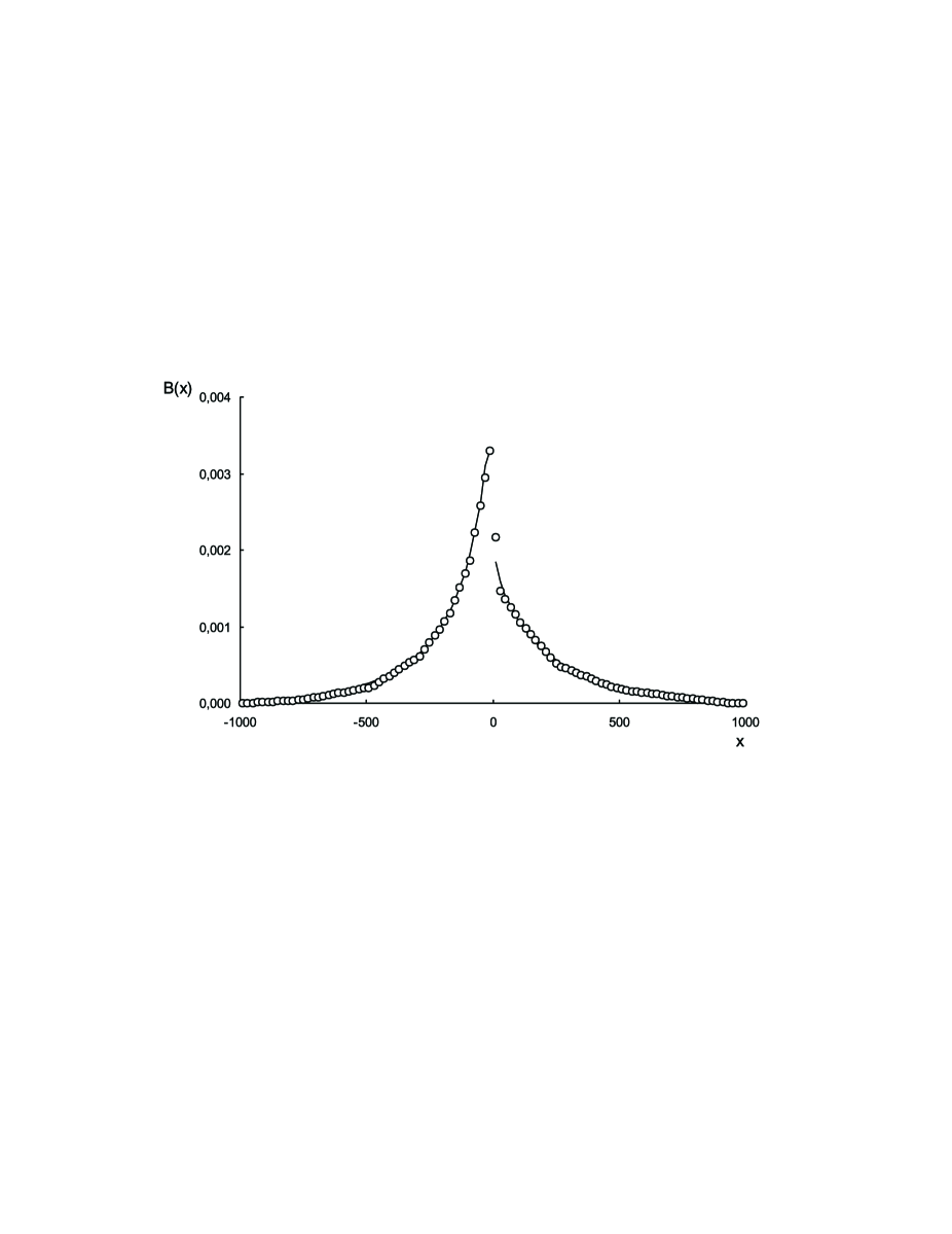
Figure 1: Branches of the strip brightness distribution for the model of a relativistic quasar’s accretion disk (solid line) and the strip brightness distribution samples restored in the numerical simulations (circles). The scale along the x axis is in units of the black hole gravitational radius $r_{g}=GM/c^{2}$ .

We considered the geometrically thin, optically thick accretion disk rotating in the prograde direction in the equatorial plane of a Kerr black hole with mass $M=10^{8}M_{\odot}$ , maximal normalized angular momentum $a=0.998$ [37] and luminosity close to the Eddington limit. The details of these calculations are given in the paper [28]. The solid line in Fig.1 shows the strip brightness distribution of our disk model $B(x)$ in the V photometric band for the angle between the rotational axis of the disk and the line of sight $i=45$. The rotation of the disk is counter-clockwise and $x$ axis is coincided with the major axis of the ellipse which is the projection of the disk onto the picture plane. The coordinate origin coincident with the center of the disk and the scale along the $x$ axis is in units of the gravitational radius $r_{g}=GM/c^{2}$, where $G$ is the gravitation constant and $c$ is the velocity of light. We set the total flux emitted by the visible surface of the disk equal to unity. The negative branch $B(x)$ in Fig.1, which correspond to the approaching edge of the disk, is clearly brighter than the receding side. Both branches - positive $B(x)$ and negative as the function $B(-x)$ can be approximated well by convex downward, monotonically non-increasing functions.

In our numerical simulations, we used for calculation the HME light curve the first version of canonical dissection, with $\xi_{i}=(x_{i}+x_{i+1})/2$, $\Delta\xi=\Delta x=20$, $\xi_{i}=-990+20(i-1)$ for $i=1,2,...M=100$ and $x_{i}=-1000+20(i-1)$ for $i=1,2,...N=101$ (both $\xi$ and $x$ in unit $r_{g}$ ). It be assumed that caustic crossing of the disk with $B(\xi)$, shown by solid line in Fig.1, is accompanied by a flux decrease. We added the noise in the form of a random Gaussian numbers with zero mean and a standard deviation equal to 1% of the maximal flux value to the initial data samples $I(x_{i})$. The resulting samples for the light curve $I_{o}(x_{i})$ for the values of the free parameters $I_{0}=0$ and $t_{0}=0$ are shown by circles in Fig.2.

We searched for the branches $B(\xi)$ and $B(-\xi)$ on the compact set of non-negative, monotonically non-increasing, convex downward functions for various $I_{0}$ and $t_{0}$ values using a modified version of the PTISR code written in FORTRAN [26,27]. To reduce the effect of roundoff errors, we transformed all real variables used in the PTISR and its auxiliary subroutines into double precision variables with 16 significant digits in their floating-point mantissas. We also used the additional a priori information that $B(\xi)$ is equal to zero at the ends of the domain of variation of the argument. This is equivalent to specifying the size of this interval, which required in the solution of any ill-posed problem. Estimating the size of the domain where $B(\xi)$ takes on nonzero values does not present difficulties in practice. Initially, a domain clearly exceeding probable values for this interval is adopted, and its size is then refined via a series of successive approximations.

It is convenient to adopt the quantity

$$\chi^{2}_{N}=\sum_{i=1}^{N}[(I_{o}(x_{i})-I_{c}(x_{i}))/\sigma_{i}]^{2},$$

for the residual, where $N$ is the number of data samples on the HME light curve $I_{o}(x_{i})$, $\sigma_{i}$ are the estimated standard errors of these samples, and $I_{c}(x_{i})$ are the fluxes corresponding to the restored strip brightness distribution. The residual had its minimum for the free parameters values $I_{0}=0.000\pm 0.001$ and $t_{0}=3.0\pm 2.0$ . The samples for the corresponding restored branches of the strip brightness distribution are shown by circles in Fig.1, and the light curve is shown by solid line in Fig.2. The minimum $\chi^{2}_{N}=50.2$ , whereas the value corresponding to a probability of 50% that the hypothesis in question should be adopted is $100.3$ for $N=101$ degrees of freedom. On the whole, the inferred free parameter values end strip brightness distribution branches are close to their initial specified values. Thus, the results of our numerical simulation show that the proposed technique is potentially a powerful tool.

4. Observational data for HMEs in components of

gravitational lens QSO 2237+0305

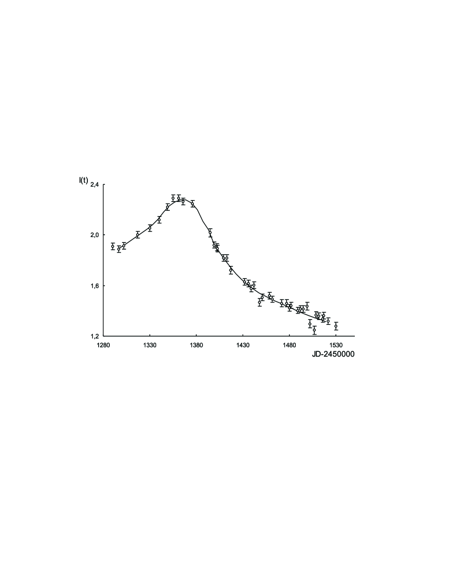
Figure 3: Samples of the HME light curve observed by the OGLE group in component C of the gravitational lens QSO 2237+0305 in V band (circles) and the light curve correspond to the restored strip brightness distribution (solid line).

The observational data of the OGLE group show that, in Summer of 1999, component C exhibited a characteristic flare, such as may occur during microlensing by a fold caustic accompanied by the disappearance of additional source images. We obtained the V magnitudes for the HME light curve and their errors via the Internet from the OGLE server and transformed these magnitudes into flux samples averaging them over each observing night and assuming that a unit level corresponds to $18^{m}.0$. These samples shown by circles in Fig.3 as a function of time expressed in modified Julian date JD - 2450000.0. The vertical line segments indicate intervals corresponding to two standard deviations $(\pm\sigma)$.

The HME in component A, observed in Autumn 1999, correspond to case when the caustic crossing leads to the appearance of additional images of the source accompanied by a sharp amplification of the flux. We obtained the V - band fluxes of component A (in millijansky, mJy) measured by the OGLE and GLITP (PSFphotII photometry) groups and their errors also via the Internet. The GLITP data, $I_{G}(t_{i})$, form a fairly dense series, but cover only the upper part oh the ascending branch and the maximum of the HME light curve. The OGLE data, $I_{O}(t_{i})$, were more sparse, but cover the lower part of the ascending branch of the curve well. Therefore, we decided to use both of these photometric series in our subsequent analysis.

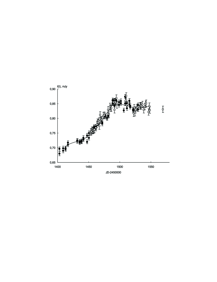
Figure 4: Samples of the HME light curve observed by the OGLE (filed circles) and GLITP (open circles) groups in component A of the gravitational lens QSO 2237+0305 in V band and the light curve correspond to the restored strip brightness distribution (solid line).

When the OGLE and GLITP photometric data plotted together, it is obvious that there is an offset between them, and that the $I_{O}(t_{i})$ values exceed the $I_{G}(t_{i})$ values measured at the same moments. Since this offset is not large, and the data obtained in each photometric system cover a fairly extensive time interval with appreciable flux variations, we decided to unify the data series by assuming a linear relation between them: $\ I_{O}(t_{i})=aI_{G}(t_{i})+b$ . The coefficients in this relation were determined from a least-squares fit with a linear interpolation of the $I_{G}(t_{i})$ values in the overlapping time interval, and were found to be $a=1.125$ and $b=-0.042$ . Figure 4 shows the flux measurements reduced to the OGLE photometric systems as a function of the modified Julian date, JD - 2450000.0 . The filled and open circles show the OGLE and GLITP observations, respectively. The vertical line segments indicate intervals corresponding to two standard deviations $(\pm\sigma)$. The flux values do not display systematic differences, and the unified series of observations is fairly uniform.

5. Results of restoration of strip brightness distributions

Since the singular nature of the main integral equation (2) requires the use of grids with canonical dissections, we again adopted the first version of such grids described above with $\Delta x=\Delta\xi$. We searched for the branches $B(\xi)$ and $B(-\xi)$ on the compact set of non-negative, monotonically non-increasing, convex downward functions for various $I_{0}$ and $t_{0}$ values. Adopting $K=1$,$\ V_{\perp}=1$ and $x=t-t_{0}$, we measure the distance $x$ and the variable of integration $\xi$ in units of time.

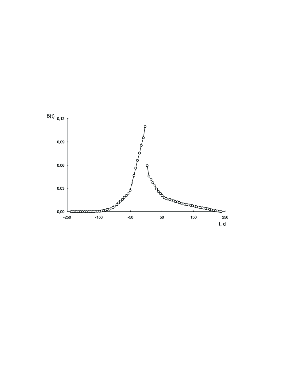
Figure 5: Branches of the strip brightness distribution across the quasar’s accretion disk restored from the analysis of observations of the HME in component C. The scale along the abscissa axis is in units of time (days).

The samples $I_{o}(x_{i})$ were computed for the observations of the HME in component C via a linear interpolation onto a uniform grid $x$ of $N=38$ values with a step $\Delta x=\Delta\xi=6^{d}.0$ in the interval $[t_{0}-96^{d},t_{0}+126^{d}]$. The search for the branches of the strip brightness distribution was carried out on the grid $\xi_{i}=-237^{d}.0+(i-1)\Delta\xi,i=1,2,...M=80$. The values of the free parameter that yielded the global minimum of the residual were $I_{0}=1.020\pm 0.005$ and $t_{0}=1392^{d}.3\pm 0^{d}.1$ . The minimum of the residual function is $\chi^{2}_{N}=22.6$, whereas the value corresponding to a probability of 50% that the hypothesis in question should be adopted is 37.3 for $N=38$ degrees of freedom. Figure 5 shows the restored branches of the strip brightness distribution. The corresponding light curve is shown by the solid line in Fig.3, and fits the observational data well.

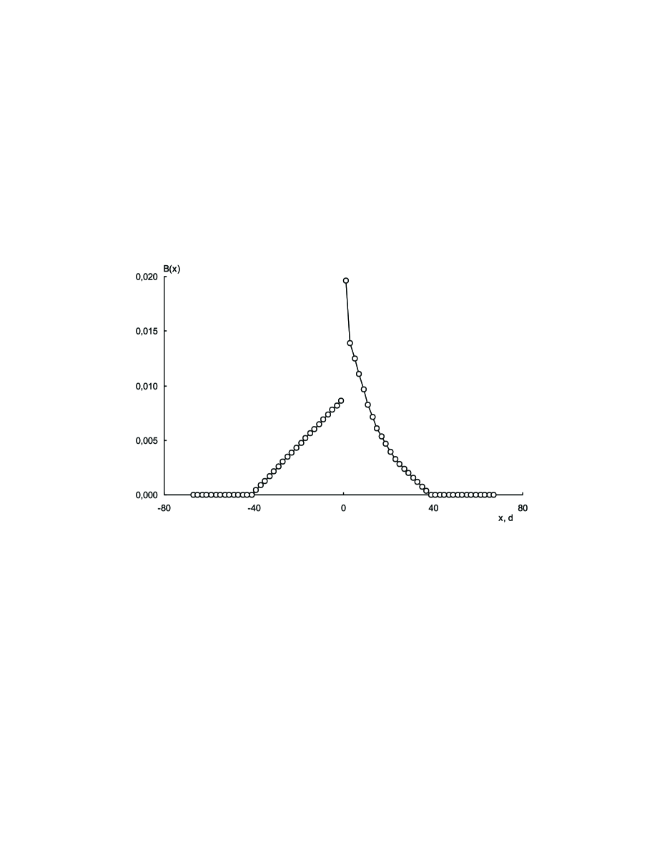
Figure 6: Branches of the strip brightness distribution across the quasar’s accretion disk restored from the analysis of observations of the HME in component A. The scale along the abscissa axis is in units of time (days).

The canonical dissections with $\Delta x=\Delta\xi=2^{d}.0$ was used for the analysis of the observations of the HME in component A. The light curve was interpolated onto a uniform grid $x_{i}$ of $N=69$ points in the interval $[t_{0}-68^{d},t_{0}+68^{d}]$. The search for the strip brightness distribution was carried out on a grid of $M=68$ points in the interval $[-67^{d},67^{d}]$. The best-fit values of the free parameters were $I_{0}=0.697\pm 0.001$ mJy and $t_{0}=1479^{d}.4\pm 0^{d}.1$. These are fairly close to the values obtained via model-fitting of the GLITP observations [23]. The values for the restored branches of the strip brightness distribution are shown by the circles in Fig.6 and the light curve corresponding to the derived brightness distribution by the solid curve in Fig.4. The minimum residual was $\chi^{2}_{N}=37.2$; the value corresponding to a 50% probability that the curve is agreement with the data for the case of $N=69$ degrees of freedom is 68.3 . Thus, the agreement with the observations is fairly good. This is confirmed in Fig.4, where we can see that the calculated light curve tracks the observed counts well. At the same time, the curve is not completely consistent with the expected shape of the lensing curve expected for a fold caustic. This is especially noticeable in the interval following the flux maximum, where a deviation from monotonic behavior is observed. This was also pointed out in connection with model-fitting of the brightness distribution [23]. It is possible that curvature of the caustic, nearness to a cusp, or the influence of other nearby caustics is manifest in this HME.

The presence of possible deviations from a simple model with a linear fold caustic is also reflected by the shape of the restored strip brightness distribution. We can see in Fig.6 that two branches differ appreciable. The shape of the positive branch is close to the expected strip brightness distribution for a relativistic accretion disk ( see Fig.1). while the negative branch forms a simple straight line segment. Nevertheless, the derived strip brightness distribution is in agreement with the results of fitting the GLITP data with a standard model for Newtonian accretion disk, whose radius in time units proved to be $39^{d}.6$ [23].

6. Estimations of sizes of accretion disk

As was already noted above, if the time for the intersection of the source by the caustic is known, the linear size of the source can be derived using the information about projection of the tangential velocity of the caustic onto the axis normal to the caustic, $V_{\perp}$. In addition, the time intersection of the accretion disk depends on the inclination of the plane of the disk to the line of sight and the direction of the motion of the caustic relative to the major axis of the ellipse corresponding to the projection of the disk onto the picture plane. Therefore, even $V_{\perp}$ is known very accurately, we can determine only a lower limit for a the linear size of the disk from the strip brightness distribution.

Let us project the spatial-velocity vectors of all the objects participating in the HME onto a plane perpendicular to the line of sight from the observer to the center of the accretion disk. We denote $\vec{V}_{s},\vec{V}_{d}$, and $\vec{V}_{o}$ to be the two-dimensional projected velocities of the source, gravitational lens, and observer, respectively. As was shown in [5], the two-dimensional vector of the projection of the velocity of the caustic onto this plane $\vec{V}$ can be written as

$$\vec{V}=\frac{\vec{V}_{s}}{1+z_{s}}-\frac{\vec{V}_{d}}{1+z_{d}}\frac{D_{s}}{D_{d}}+\frac{\vec{V}_{o}}{1+z_{d}}\frac{D_{ds}}{D_{d}}\ ,$$

where $z_{s}$ and $z_{d}$ are the redshifts of the quasar and the gravitational lens, and $D_{s},D_{d}$ , and $D_{ds}$ are the angular diameter distances between the observer and quasar, the observer and lens, and the lens and quasar, respectively. For the parameters of the gravitational lens QSO 2237+0305 ($z_{s}=1.695,z_{d}=0.0394$) and reasonable velocities for the motions involved, the second term in (5) is the determining one. Therefore, we can obtain for the velocity with which the source is scanned by the caustic

$$V_{\perp}\approx\frac{V_{\perp,d}}{1+z_{d}}\frac{D_{s}}{D_{d}}\ ,$$

where $V_{\perp,d}$ is the projection of $\vec{V}_{d}$ onto the local normal to caustic.

The precise value of $V_{\perp}$ is not known. A statistical analysis of the peculiar velocities of galaxies yielded the mean value 663 km/s, while the range of the projected velocity $V_{\perp,d}$ for 90% confidence interval was roughly $100\leq V_{\perp,d}\ (km/s)\leq 1000$ [25]. The distances $D_{d}$ and, especially, $D_{s}$ in (6) is depend on cosmological parameters. Taking into account possible variations of models of Universe from the usual ($\Omega_{0}=1$) to the model with a dominance of the vacuum energy consistent with modern observational data ($\Omega_{0}=0.3,\lambda_{0}=0.7$), the interval of possible caustic-scanning velocities $V_{\perp}$ becomes $765\leq V_{\perp}\ (km/s)\leq 10548$ [25].

If we formally adopt a value of the velocity in the middle of this interval, $V_{\perp}=5600\ km/s$, then we can estimated the sizes of the accretion disk. The intersection time for the profile of the strip brightness distribution from the HME in component C (see Fig.5) is roughly $300^{d}$, which corresponds to a linear size of $1.5\times 10^{16}$ cm, or $4.7\times 10^{-3}$ pc. This time from the HME in component A (see Fig.6) is $80^{d}$, which correspond a size $3.9\times 10^{15}$ cm, or $1.3\times 10^{-3}$ pc. The difference of the sizes is not very large. It is possible that this difference could be explained by either a difference of $V_{\perp}$, or by the different direction of the caustic’s motion relative to the major axis of the ellipse corresponding to the projection of the accretion disk onto the picture plane.

7. Conclusions

Our proposed technique for the successive restoration of the branches of the strip brightness distribution of a quasar accretion disk via analysis of observations of the HME makes it possible to take into account a large amount of a priori information that consistent with the physics of the phenomena. This ensures that the resulting solution is accurate and stable against a random noise. Both branches of the strip brightness distribution can be derived from the light curve without applying any rigid model constraints. These properties are confirmed by numerical simulations and results obtained by applying the technique to real observational data.

We have analyzed the HMEs in components C and A of the gravitational lens QSO 2237+0305 observed by the OGLE and GLITP groups using our model-independent technique. This analysis has yielded the estimations of the form of the strip brightness distribution across the accretion disk. The results for the HME in component C are consistent with the hypothesis that we have observed a scan of the source by a fold caustic. The form of the strip brightness distribution corresponds to our expectation for a relativistic accretion disk rotating around a supermassive black hole. In spite of a small value of residual $\chi^{2}_{N}$, the features in the light curve for the HME in component A and the restored strip brightness distribution suggest that the disk was not scanned by simple linear fold caustic. It is possible that curvature of the caustic, nearness to a cusp, or the influence of other nearby caustics is manifest in the details of the light curve for this HME.

The sizes of sources, measured in units of time, $300^{d}$ for the HME in component C and $80^{d}$ for the HME in component A, are consistent with the results of model-fitting. The crude estimates for the linear sizes are $1.5\times 10^{16}$ cm and $3.9\times 10^{15}$ cm, respectively. This difference could be due to a difference in either the scanning velocity, or the direction of the caustic’s motion relative to the major axis of the elliptical projection of the quasar’s accretion disk onto the picture plane.

8. Acknowledgements

The authors thank the OGLE and GLITP groups for the opportunity to obtain the observational material used in this study.

This work was partially supported by the Federal Science and Technology Program ”Astronomy”, the Russian Foundation for Basic Research (project code 02-02-17524), and the program ”Universities of Russia”.

References

1. J.H.Krolik, Active galactic nuclei (Princeton: Princeton University Press, 1999).

2. B.M.Peterson and K.Horne, Astron. Nachrichten. 325, 248 (2004)

3. N.White, Nature 407, 146 (2000).

4. B.Paczynski, Astrophys. J. 301, 503 (1986).

5. R.Kayser, S.Refsdal, and R.Stabell, Astron. and Astrophys. 166, 36 (1986).

6. B.Grieger, R.Kayser, and T.Schramm, Astron. and Astrophys. 252, 508 (1991).

7. E.Agol and J.Krolik, Astrophys. J. 524, 49 (1999).

8. S.Mineshige and A.Yonehara, Publ. Astron. Soc. Japan. 51, 497 (1999).

9. M.J.Irwin, R.L.Webster, P.C.Hewitt, et al., Astron. J. 98, 1989 (1989).

10. K.P.Rauch, and R.D.Blandford, Astrophys. J. 381, L39 (1991).

11. M.Jaroszynski, J.Wambsganss, and B.Paczynski, Astrophys. J. 396, L65 (1992).

12. R.T.Corrigan, M.J.Irwin, J.Arnaud, et al., Astron. J. 102, 34 (1991).

13. R.Ostensen, S.Refsdal, R.Stabell, et al., Astron. and Astrophys. 309, 590 (1996).

14. V.G.Vakulik, V.N.Dudinov, A.P.Zheleznyak, et al., Astron. Nachr. 318, 73 (1997).

15. R.W.Schmidt, T.Kundic, U.-L.Pen, et al., Astron. and Astrophys. 392, 773 (2002).

16. P.R.Wozniak, C.Alard, A.Udalski, et al., Astrophys. J. 529, 88 (2000).

17. P.R.Wozniak, A.Udalski, M.Szymanski, et al., Astrophys. J. 540, 65 (2000).

18. J.S.B.Wyithe, R.L.Webster, E.L.Turner, and D.J.Mortlock, Monthly Notices Roy. Astron. Soc. 315, 62 (2000).

19. J.S.B.Wyithe, R.L.Webster, and E.L.Turner, Monthly Notices Roy. Astron. Soc. 318, 1120 (2000).

20. V.N.Shalyapin, Astron. Lett. 27, 150 (2001).

21. A.Yonehara, Astrophys. J. 548, L127 (2001).

22. D.Alcalde, E.Mediavilla, O.Moreau, et al., Astrophys. J. 572, 729 (2002).

23. V.N.Shalyapin, L.J.Goicoechea, D.Alcalde, et al., Astrophys. J. 579, 127 (2002).

24. N.I.Shakura and R.A.Sunyaev, Astron. and Astrophys. 24, 337 (1973).

25. L.J.Goicoechea, D.Alcalde, E.Mediavilla, and A.Munoz, Astron. and Astrophys. 397, 517 (2003).

26. A.N.Tikhonov, A.V.Goncharsky, V.V.Stepanov, and A.G.Yagola, Regularizing algorithms and a priori information (Nauka, Moscow, 1983) [in Russian].

27. A.M.Cherepashchuk, A.V.Goncharsky, and A.G.Yagola, Ill-posed problems in astrophysics (Nauka, Moscow, 1985) [in Russian].

28. M.B.Bogdanov and A.M.Cherepashchuk, Astron. Rep. 46, 626 (2002).

29. M.B.Bogdanov and A.M.Cherepashchuk, Astron. Rep. 48, 261 (2004).

30. P.Schneider, J.Ehlers, and E.E.Falco, Gravitational lenses (Berlin: Springer, 1992).

31. A.F.Zakharov, Gravitational lenses and microlenses (Yanus-K, Moscow, 1997) [in Russian].

32. B.S.Gaudi and A.O.Petters, Astrophys. J. 574, 970 (2002).

33. S.M.Belotserkovsky and I.K.Lifanov, Numerical methods for singular integral equations and their applications to aerodynamics, elasticity theory, and electrodynamics (Nauka, Moscow, 1985) [in Russian].

34. M.B.Bogdanov, arXiv: astro-ph/0102031 (2001).

35. I.D.Novikov and K.S.Thorne, Black Holes (New York: Gordon and Breach, 1973). P.343.

36. D.N.Page and K.S.Thorne, Astrophys. J. 191, 499 (1974).

37. K.S.Thorne, Astrophys. J. 191, 507 (1974).

Figure 2: Samples for the model HME light curve with noise superimposed (circles) and the curve correspond to the restored strip brightness distribution (solid line). The units along x axis are the same as in Fig.1.