Full characterization of binary-lens event OGLE-2002-BLG-069 from PLANET observations

We analyze the photometric data obtained by PLANET and OGLE on the caustic-crossing binary-lens microlensing event OGLE-2002-BLG-069. Thanks to the excellent photometric and spectroscopic coverage of the event, we are able to constrain the lens model up to the known ambiguity between close and wide binary lenses. The detection of annual parallax in combination with measurements of extended-source effects allows us to determine the mass, distance and velocity of the lens components for the competing models. While the model involving a close binary lens leads to a Bulge-Disc lens scenario with a lens mass of $M=(0.51\pm 0.15)\leavevmode\nobreak\ M_{\odot}$ and distance of $D_{\rm{L}}=(2.9\pm 0.4)\leavevmode\nobreak\ {\rm{kpc}}$, the wide binary lens solution requires a rather implausible binary black-hole lens ($M\gtrsim 126\leavevmode\nobreak\ M_{\odot}$). Furthermore we compare current state-of-the-art numerical and empirical models for the surface brightness profile of the source, a G5III Bulge giant. We find that a linear limb-darkening model for the atmosphere of the source star is consistent with the data whereas a PHOENIX atmosphere model assuming LTE and with no free parameter does not match our observations.

1 Introduction

By exploiting the phenomenon of the bending of light from background source stars due to the gravitational field of intervening compact objects acting as lenses, Galactic microlensing provides an opportunity to infer the brightness profile of the source star, the mass and configuration of the lens, as well as the relative parallax and proper motion. In recent years there has been a remarkable increase in the power of microlensing survey alert systems like OGLE-III (Udalski 2003) and MOA (Bond et al. 2001). As a consequence, binary-lens microlensing events have become a unique and valuable tool to study, in unprecedented detail, members of the source and lens population within our Galaxy and in the Magellanic Clouds (Abe et al. 2003; Fields et al. 2003; An et al. 2002b; Albrow et al. 2001b, 2000a, 2000b, 1999a, 1999b, 1999c). The OGLE-2002-BLG-069 event is an ideal example for showing the current capabilities of microlensing follow-up observations.
The passage of a source star over a line-shaped (fold) caustic as created by a binary lens produces a characteristic peak in the light curve which depends on the stellar brightness profile. The data obtained for OGLE-2002-BLG-069 clearly reveal a pair of such passages consisting of an entry and subsequent caustic exit, where the number of images increases by two while the source is inside the caustic.
This binary-lens event is the first where both photometric and high-resolution spectroscopic data were taken over the whole course of the caustic exit. The previous attempts on EROS-2000-BLG-5 (Afonso et al. 2001) had good coverage but low spectral resolution (Albrow et al. 2001a), or a pair of spectra taken with high resolution but low signal-to-noise (Castro et al. 2001). Prior to this study, we presented a fold-caustic model of the OGLE-2002-BLG-069 photometric data comparing a linear law and a model derived from PHOENIX v2.6 synthetic spectra for the limb-darkening and analyzed variations in the $\@element{\mathrm{H}}\alpha$ line as observed in high-resolution UVES spectra taken over the course of the caustic passage (Cassan et al. 2004). A full account of the spectral observations in $\@element{\mathrm{H}}\alpha,\leavevmode\nobreak\ \@element{\mathrm{H}}\beta$, $\@element{\mathrm{CaII}}$, $\@element{\mathrm{Mg}}$ and other lines will be given in Beaulieu et al. (2005). Here, we concentrate on the photometric data alone in order to present the full binary-lens model.
For the majority of observed microlens events all information about lens mass, relative lens-source distance and proper motion is convolved into one single characteristic time scale. Binary-lens events however are especially sensitive to effects caused by finite source size and parallax, so that in combination with the determination of the angular source radius, these three lens quantities can be measured individually (Refsdal 1966; Gould 1992). This is only the second binary microlensing event, after EROS-BLG-2000-5 (An et al. 2002a), for which this has been achieved. Despite our high sampling rate and the small uncertainty of our photometric measurements, we still encounter the well known close/wide-binary ambiguity originating in the lens equation itself (Dominik 1999) and which may only be broken with additional astrometric measurements as proposed in Dominik (2001) and Gould & Han (2000).

2 OGLE-2002-BLG-069 photometry data

Alerted by the OGLE collaboration (Udalski 2003) on June 1 2002 about the ongoing Bulge microlensing OGLE 2002-BLG-069 event (R.A.=$17^{h}48^{m}1^{s}.0$ , decl.= $-21^{\circ}16^{\prime}9^{\prime\prime}.3$), the PLANET collaboration network began photometric observations on June 18, using 6 different telescopes, namely SAAO 1m (South Africa), Danish 1.54m (La Silla), ESO 2.2m (La Silla), Canopus 1m (Tasmania), Stromlo 50” (Australia) and Perth 1m (Australia). Data were taking in $I$- (UTas, Danish, SAAO, Perth), $R$- (La Silla) and $V$-bands (Stromlo). Since the $V$-band data set of Stromlo contains only 8 points, which is less than the number of parameters we fit, we do not use it in the modeling process.
The photometry reductions were done by point-spread-function (PSF) fitting using our own modified version of DoPHOT (Schechter et al. 1993), implemented as part of the PLANET reduction pipeline. The full raw data set including the public OGLE data (available from www.astrouw.edu.pl/$\sim$ogle/ogle3/ews/ews.html) consists of 675 points. Data that were obviously wrong according to the observational log books or for which the reduction software did not succeed in producing a proper photometric measurement have been eliminated. Moreover, PLANET data taken under reported seeing that was significantly above the typical value for the given site were removed according to the cut-offs listed in Table 1. Altogether about 2 % of the data were rejected, leaving us with a total of 651 points (Fig.1).

telescope	median seeing	seeing cut	number of
	(arcsec)	(arcsec)	points
ESO 2.2m	1.13	$\leq$ 2.5	150
Danish	1.62	$\leq$ 2.5	108
UTas	3.13	$\leq$ 3.6	58
SAAO	1.93	$\leq$ 2.6	153
Perth	2.43	$\leq$ 2.8	86

Table 1: Selection criteria for PLANET photometric dataset.

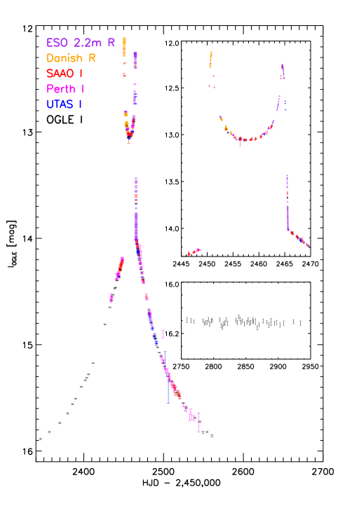
Figure 1: Complete photometric I- and R-band datasets of PLANET and OGLE, with PLANET calibrated to the OGLE filter. The upper inner panel shows a zoom of the caustic passages, while the lower panel displays the baseline measurements of OGLE made in the 2003 season, i.e. one year after the lensing event occurred.

Thanks to the favourable brightness at baseline ($I_{\rm{OGLE}}=16.15\pm 0.01$ mag) and low crowding of this event, the correlation between seeing and observed flux is negligible and does not yield a significant signature in the data, contrary to some previously analyzed events (e.g. Albrow et al. 2000b).

3 Binary-lens model

3.1 Parametrization and general approach

The art of binary-lens light curve modeling still poses significant challenges. A priori the parameters have a large dynamical range ( the mass ratio for instance can vary over several magnitudes) and the standard $\chi^{2}$ goodness-of-fit measure of the complicated high-dimensional parameter space is very sensitive to subtle changes in most of the parameters. Furthermore the parameter space contains both real ambiguous solutions and false numerical minima where parts of the $\chi^{2}$ surface are either flat or contain very irregular and rough regions, in which local optimizing codes, based on gradient search algorithms (Press et al. 1992), can get trapped. Another barrier is the treatment of extended-source effects, which are prominent when the source is resolved by caustic crossings. Given the large number of initial model parameters and the large number of data points, all suggested methods of calculate binary-lens curves of extended sources (Kayser & Schramm 1988; Dominik 1995; Wambsganss 1997; Dominik 1998a) are too time consuming to be used for the complete data set. Therefore we employ a strategy similar to that used by Albrow et al. (1999a). We treat the data obtained during the caustic passage(s) separately from the remainder of the light curve using the criteria given below.

For a caustic crossing binary-lens event a minimum of $7+2n$ parameters are required, namely $t_{0},u_{0},t_{\rm{E}},q,d,\alpha$, and $\rho_{\ast}$, plus $F_{\rm{S}}$ and $F_{\rm{B}}$ for each of the $n$ different observing sites (here $n=6$). Here $t_{0}$ denotes the time of closest approach to the center of mass of the binary, $u_{0}\geq 0$ the impact parameter at time $t_{0}$, $t_{E}$ is the time needed to cross the angular Einstein radius, which is defined as

$$\theta_{\rm{E}}=\sqrt{\frac{4GM}{c^{2}}\frac{D_{\rm{LS}}}{D_{\rm{L}}D_{\rm{S}}}}\;,$$ (1)

where $D_{\rm{L}},D_{\rm{S}}$ and $D_{\rm{LS}}$ are the observer-lens, observer-source, lens-source distances and $M$ the total mass of the binary lens. The lens is characterized by the mass ratio $q=m_{2}/m_{1}$ between the secondary and the primary and their angular separation $d\,\theta_{\mathrm{E}}$. The impact angle $\alpha$ is measured between the line from the secondary to the primary and the positive direction of source motion relative to the lens. The angular source size is given by $\rho_{\star}\,\theta_{\mathrm{E}}$. The flux of the unlensed source star is $F_{\rm{S}}$ and $F_{\rm{B}}$ is the flux contribution of any other unlensed sources (including the lens) within the aperture. For every observing site, $F_{\rm{B}}$ and $F_{\rm{S}}$ are determined independently to account for different background and flux characteristics of the individual telescopes/detectors. Modeling the parallax effect due to the orbital motion of the Earth requires 2 more parameters, the length $\pi_{\rm{E}}$ of the semi-major axis projected onto the sky plane and a rotation angle $\psi$, describing the relative orientation of the transverse motion of the source track to the ecliptic plane. The source surface brightness profile in this study is described by either a 1- or 2-parameter law so that the complete photometric model consists of up to 23 parameters.
Our initial search for the lens model involves only data outside the caustic-crossing region, where extended-source effects are negligible. Moreover, we also neglect parallax effects. We then scan the parameter space on a grid of fixed values of mass ratio $q$ and lens separation $d$, optimizing the remaining parameters $t_{0},u_{0},t_{\rm{E}}$ and $\alpha$ with the genetic algorithm Pikaia (Charbonneau 1995; Kubas et al. 2005) and subsequently with a gradient routine to obtain $\chi^{2}$-maps such as shown in Fig. 2, which give an overview of possible model solutions. The values of $F_{\rm{S}}$ and $F_{\rm{B}}$ are simultaneously computed by inexpensive linear fitting. To explore in more detail the minima that are found we conduct a search with Pikaia over a restricted range of $q$ and $d$ but this time allowing these parameters to be optimized as well and again use gradient based techniques for final refinement. The results from the fold-caustic-crossing modeling in combination with the point source fits are then used to generate magnification maps with the ray-shooting technique (Wambsganss 1997). These maps contain the full information on the lens-source system.
We note that in crowded fields the raw photometry errors given by the reduction process clearly underestimate the true errors (Wozniak 2000). To achieve a reduced $\chi^{2}$ of unity in our best fit model the photometric error bars would have to be rescaled by factors of 1.51 (SAAO), 1.92 (UTas), 1.34 (Danish), 1.16 (ESO 2.2m), 1.59 (Perth) and 2.3 (OGLE).

3.2 Preferred lens parameters

To exclude the data points which are affected by finite source effects we apply the argument given in Albrow et al. (1999a). There it was shown, that for times $\gtrsim 3\Delta t$ away from the fold caustic, where $\Delta t$ is the time in which the source radius crosses the caustic, the point source approximation is accurate enough for photometric errors of $\lesssim 1\%$. Based on the measured caustic crossing times (see section 4) we cut out data between $2450.0\leq$ HJD’ $\leq 2452.8$ and $2463.0\leq$ HJD’ $\leq 2466.0$, where $\mbox{HJD'}=\mbox{HJD}-2450000$. We then search for promising regions in parameter space on a grid of mass ratio $q$ and lens separation $d$, the two parameters that characterize the binary lens, with $q=0.01,0.05,0.10,0.15,...,1.00$ and $d=0.01,0.05,0.10,0.15,...,4.70$. The result is shown in Fig. 2.

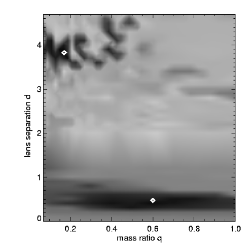
Figure 2: Gray-scale $\chi^{2}$ map of full grid in mass ratio q and lens separation d, with darker regions representing lower values of $\chi^{2}$. The irregularity of parameter space is reflected by the patchy appearance of the map, especially around the wide binary model in the upper left part of the plot. The best models are marked by the white diamonds at $q\sim$ 0.6,  $d\sim$ 0.5 (close binary) and at $q\sim$ 0.16, $d\sim$ 3.7 (wide binary).

While the apparent close binary solution around $q\sim$ 0.6 and $d\sim$ 0.5 seems to be well defined, the numerical routines converge poorly in the vicinity of the wide-binary solution, reflecting the intricacy of binary-lens parameter space. By bracketing apparently interesting subsets of the $(q,d)$ plane, our optimization algorithm identifies the best wide solution at $q\sim$ 0.16 and $d\sim$ 3.7.

Figure 3: The coordinates $(\tilde{x},\tilde{y})$ are chosen so that the right hand system $(\tilde{x},\tilde{y},\tilde{z})$ fulfils $\tilde{x}=z,\;\tilde{y}=y,\;\tilde{z}=-x$ for $\varphi=\chi=\psi=0$. The longitude $\varphi$ is measured from the perihelion $t_{p}$ towards the Earth’s motion and the latitude $\chi$ from the ecliptic plane towards ecliptic north.

3.3 Annual parallax

Close-binary-lens models that neglect the motion of the Earth around the Sun show a significant asymmetry in the residuals which disappears if parallax is taken into account. Adapting the convention in Dominik (1998b) and illustrated in Fig. 3 we introduce as a parameter the projected length $\pi_{\rm{E}}$ of the Earth’s semi-major axis in the sky plane, which is defined as

$$\pi_{\mathrm{E}}=\pi_{\mathrm{LS}}/\theta_{\mathrm{E}}=\frac{1\leavevmode\nobreak\ {{\rm{AU}}}}{\theta_{\mathrm{E}}}\,\left(\frac{1}{D_{\mathrm{L}}}-\frac{1}{D_{\mathrm{S}}}\right)\,,$$ (2)

where $\pi_{\mathrm{LS}}$ is the relative lens-source parallax. The second additional parameter is the angle $\psi$ describing the relative orientation of the source motion to the ecliptic. The heliocentric ecliptic coordinates $(\varphi,\chi)$ used for the parallax modeling are derived from the standard geocentric ecliptic coordinates $(\lambda,\beta)$ by applying $\chi=\beta$ and $\varphi=\lambda+\pi+\varphi_{\gamma}$, where $\varphi_{\gamma}$ is the angle of the vernal equinox measured from the perihelion.
In 2002 Earth reached the perihelion at $\sim$ 2277.1 HJD’ and the time of the vernal equinox was $\sim$ 2354.3 HJD’. This yields $\varphi=163.3^{\circ}$ and $\chi=2.1^{\circ}$ for OGLE-BLG-2002-069.

4 Source model

The data taken when the source transits the caustic show the corresponding characteristic shape. The caustic entry is not well sampled, because in the early stage of the event it was difficult to distinguish between a binary and a single lens, and the practically unpredictable rise of the light curve was rather short. On the other hand, the caustic exit has very good coverage thanks to our predictive online modeling. Hence, we focus our study on the caustic exit. We estimate that the exit occurred for ($2463.45\leq\mbox{HJD'}\leq 2467$) approximately. The corresponding subset of data comprises 95 points from ESO 2.2m, 21 points from SAAO and 17 points from UTas, giving a total of 133 points. We assume the source to move uniformly and neglect the curvature of the caustic as well as the variation of its strength on the scale of the source size. This approximation (which is justified in Sec. 5) allows us to increase computational efficiency significantly by using a fold-caustic-crossing model (e.g. Cassan et al. 2004). We recall that during a caustic crossing, the total magnification $A^{(s)}$ of the source is the sum of the magnifications of the two critical images and the three other images :

$$A^{(s)}=a_{\mathrm{crit}}\ G_{\mathrm{f}}\left(\frac{t_{\mathrm{f}}-t}{\Delta t}\ ;\ \xi^{(s)}\right)+a_{\mathrm{other}}\ \left[1+\omega(t-t_{\mathrm{f}})\right].$$ (3)

Here $\Delta t$ is the time needed for the radius of the source to cross the caustic, $t_{\mathrm{f}}$ is the date at which the limb exits the caustic and $G_{\mathrm{f}}$ is a characteristic function (Schneider & Wagoner 1987) depending on the surface brightness profile $\xi$. The blending parameters and the baseline magnitudes for each site are derived from the point-source model on the non-caustic-crossing part of the light curve ; they are held fixed in the following.
Limb-darkening is frequently characterized by a sum of power-laws:

$$\frac{\xi(\mu)}{\xi_{0}}=1-\sum\limits_{i}a_{i}(1-\mu^{i}),$$ (4)

where $\mu=\cos\,\vartheta$ is the cosine of the emergent angle of the light ray from the star, and $a_{i}\leavevmode\nobreak\ (i={1/2,1,3/2,2...}$) are the so-called limb darkening coefficients (LDC). We investigate the two most popular realizations : the linear ($a_{1}\neq 0$) and square root limb darkenings ($a_{1}\neq 0$ and $a_{1/2}\neq 0$). Performing a $\chi^{2}$ minimization on our fold-caustic data provides us with the parameters listed in Table 2 that best describe our photometric data. The value of $\chi^{2}/\mathrm{d.o.f.}$ tells us about the relative goodness of the fits among the studied models. Claret (2000) also introduced a 4-parameter law which fits the limb-darkening curves derived from spherical atmosphere models. However, as pointed out by Dominik (2004a), for coefficients beyond the linear law, the differences in the light curve are much smaller than the differences in the profiles, and it is not possible to find a unique set of coefficients given our data set. Finally, we also consider a PHOENIX atmosphere model that resulted from a spectroscopic analysis of the source star by Cassan et al. (2004), where corresponding broad-band brightness profiles for $\mathrm{R}$- and $\mathrm{I}$-band were computed.
In the upper panel of Fig. 4, the best model (with square-root limb darkening) is plotted with the data. The fit residuals obtained with the linear, square-root and PHOENIX limb darkening are displayed in the lower panels.

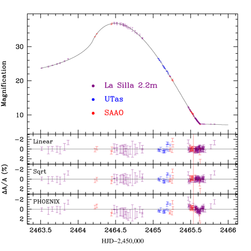
Figure 4: Data points and light curve obtained with square-root limb darkening (upper panel), and residuals coming from the linear, square-root and PHOENIX laws.

With free limb-darkening coefficients, even the linear law describes the data reasonably well, while the square-root law allows a better match. In contrast the parameter-free PHOENIX model computed assuming LTE fails. The residuals for the caustic-crossing region show systematic trends that are typical for an inappropriate limb-darkening profile, as discussed by Dominik (2004b). A new analysis taking into account NLTE effects will be done in a forthcoming paper.

Table 2: Limb-darkening coefficients (LDC) derived from the fit of OGLE-2002-BLG-069 during the caustic exit. Each set of LDC corresponds to the best fit obtained (no error rescaling here) by using the LDC as well as the fold-caustic model parameters as free parameters.

	Linear	Square root	PHOENIX
$t_{\mathrm{f}}$ (days)	$2465.624$	$2465.626$	$2465.636$
$\Delta t$ (days)	$0.71$	$0.72$	$0.72$
${\omega}$ (days-1)	$-0.10$	$-0.10$	$-0.11$
$a_{\mathrm{crit}}$	$19.98$	$20.03$	$19.85$
$a_{\mathrm{other}}$	$7.33$	$7.35$	$7.33$
$a_{1}$	$0.62$	$0.10$	-
$a_{1/2}$	-	$0.80$	-
$\chi^{2}/\mathrm{d.o.f.}$	$2.230$	$1.937$	$3.528$

In the following sections, we will use the square-root limb darkening to describe the source star.

5 A complete model

With the point-source model and the brightness profile of the source determined from the data in the caustic-crossing region, we can now derive a complete and consistent model of the lens, yielding its mass $M$, distance $D_{\rm{L}}$ and relative transverse velocity $v$. This is done by generating magnification maps with the ray-shooting method (Wambsganss 1997) for the best-fit values found for mass ratio $q$ and lens separation $d$ and then convolving these maps with the source profile modeled in section 4. The maps and the corresponding light curves derived from them, are shown in figures 5, 6, and 7.
These maps also serve as a check on the validity of the straight-fold-caustic approximation (see Sec. 4). We find that the effect of curvature of the caustic is negligible and does not influence the results of the stellar surface brightness modeling. Table 3 lists all fit parameters for the best close- and wide-binary solution. The quoted 1-$\sigma$ error bars correspond to projections of the hypersurfaces defined by $\Delta\chi^{2}=\chi^{2}-\chi^{2}_{\mathrm{min}}=1$ onto the parameter axes.

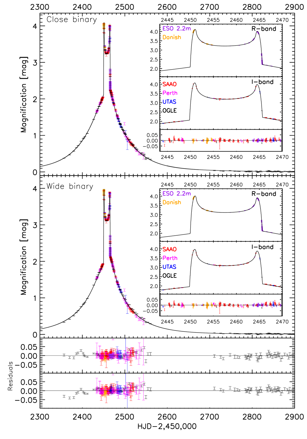
Figure 5: Lightcurves of close and wide binary-lens models and their residuals. Insets show a zoom of the caustic passages in the two different bands taken.

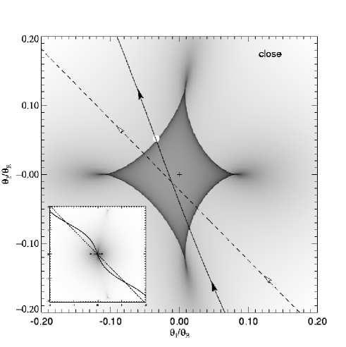
Figure 6: Magnification map and source trajectory for the close-binary model. The solid curve is the track of the source including annual parallactic motion and the dashed line represents the source motion (with direction indicated by the arrows) as seen from the Sun. The origin marked with the cross is the center of mass and the filled white circle indicates the source size. The grey-scale marks the magnification scale in the source plane, with dark regions corresponding to high magnification and bright regions referring to low magnification. The inset shows the full caustic topology, with the two filled black circles marking the positions of the binary lens components.

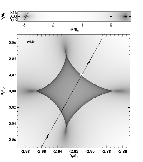
Figure 7: Magnification map and source trajectory for the wide-binary. The effect of parallax is negligible. The top panel shows the full caustic topology, where the lens positions are marked with the black filled circles and the center of mass by the cross. In the zoom around the secondary lens, lower panel, the filled white circle marks the source size, the arrows indicate the direction of source motion. As in Fig. 6 dark regions mark high magnification and bright regions represent low magnification areas.

5.1 Physical lens properties

The measured finite source size and the parallax effect yield two independent constraints for determining the lens mass $M$, its distance $D_{\rm{L}}$ and transverse velocity $v$. Assuming a luminous lens we can put upper limits on its mass using our knowledge of the absolute luminosity and distance of the source star. These were determined in Cassan et al. (2004) from spectroscopic measurements combined with the measured amount of blended light (which includes any light from the lens) inferred from the light curve modeling.
Fig. 8 plots the implied blend fraction $h=F_{\rm{B}}/(F_{\rm{S}}+F_{\rm{B}})$ if both components of the lens are main-sequence stars (from A0 to M9, Allen 1972) put at distances of $2,4,6$, and $9$ kpc along the line of sight to the lens in comparison with the blend fractions derived from OGLE data. If we assume the lens is the only source of the blended light, the inferred blend fraction from our best fit models gives an upper limit for the total lens mass of $\sim 2.5\leavevmode\nobreak\ {\rm{M}}_{\odot}$ for the close-binary and $\sim 0.8\leavevmode\nobreak\ {\rm{M}}_{\odot}$ for the wide-binary-lens model.

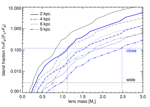
Figure 8: Assuming the lens to be composed of two main-sequence stars according to each of our models, the blend fraction $h=F_{\rm{B}}/(F_{\rm{S}}+F_{\rm{B}})$ for OGLE data (horizontal solid lines) yields upper limits (vertical dashed lines) on the total lens mass for the known brightness and distance of the source ($M_{V}=+0.9$, $(V-I)=0.95)$ and $D_{\rm{S}}=(9.4\pm 1.4)$ kpc from Cassan et al. (2004). While the close-binary model is compatible with lens masses up to $\sim 1.1-2.5\;{\rm{M}}_{\odot}$, the wide-binary model only allows lens masses up to $\sim 0.3-0.8\;{\rm{M}}_{\odot}$ for lens distances between 2-9 kpc (where the thin lines represent the wide binary lens and the thick lines the close binary lens).

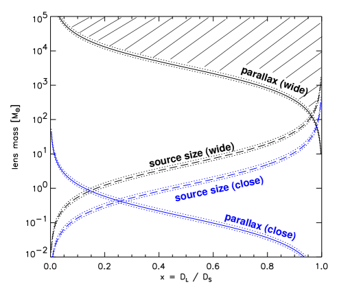
Figure 9: The independent constraints on the lens mass from the source size (dashed line) according to Eq. (6) and from parallax effects according to Eq. (7) (solid line) for the close and wide separation binary models as function of $x=D_{\rm{L}}/D_{\rm{S}}$. The dotted lines mark the uncertainty due to the error in the source distance measurement. While the close-binary constraints intersect at the plausible lens mass of $(0.51\pm 0.15)\leavevmode\nobreak\ {\rm{M}}_{\odot}$ implying a disc lens at $D_{\rm{L}}=(2.9\pm 0.4)\leavevmode\nobreak\ {\rm{kpc}}$, the wide binary favours a rather implausible scenario of a binary black hole of $M\gtrsim(126\pm 22)\leavevmode\nobreak\ M_{\odot}$ in the Bulge at $D_{\rm{L}}\gtrsim(9.0\pm 2.3)\leavevmode\nobreak\ {\rm{kpc}}$, with the hatched region marking the allowed parameter space for the wide-binary solution.

We use the source radius caustic crossing time $\Delta t$ from the straight-fold-caustic model, together with the lens geometry given by $(q,d)$ and time-scale $t_{\rm{E}}$ from the point source model, to derive the relative angular source size $\rho_{\ast}$, which expressed as a fraction of the angular Einstein radius reads

$$\rho_{\ast}=\frac{\Delta t}{t_{\rm{E}}}\;\rm{sin}\phi\;,$$ (5)

with $\phi$ being the angle between source track and caustic tangent. The source size parameter $\rho_{\ast}$ is refined by fitting on a grid of magnification maps convolved with different source sizes. So with the inferred physical source size of $R_{\ast}\simeq 10\leavevmode\nobreak\ R_{\odot}$ and source distance $D_{\rm{S}}=(9.4\pm 1.4)\;\rm{kpc}$ from the spectral measurements (Cassan et al. 2004) the constraint on the lens mass from extended-source effects can be inferred from

$$\frac{M(x)}{M_{\odot}}=\frac{{c^{2}}}{4GM_{\odot}D_{\rm{S}}}\frac{{R_{\ast}}^{2}}{{\rho_{\ast}}^{2}}\frac{x}{1-x}\;,$$ (6)

with $x=D_{\rm{L}}/D_{\rm{S}}$. The dependence of the lens mass upon annual parallax effects reads

$$\frac{M(x)}{M_{\odot}}=\frac{c^{2}}{4GM_{\odot}D_{\rm{S}}}\left(\frac{1\leavevmode\nobreak\ {\rm{AU}}}{\pi_{\rm{E}}}\right)^{2}\frac{1-x}{x}\leavevmode\nobreak\ \leavevmode\nobreak\ .$$ (7)

The curves arising from these two relations are plotted in Fig. 8 for our best fit parameters $\pi_{\rm{E}},\rho_{\ast}$ (see Table 3) of the wide and close binary-lens model. From this we obtain the following physical lens parameters,

$$M_{\rm{close}}=(0.51\pm 0.15)\leavevmode\nobreak\ M_{\odot}\;,\;{\rm{at}}\;D_{\rm{L}}=(2.9\pm 0.4)\leavevmode\nobreak\ \rm{kpc}\;$$ (8)

and

$$M_{\rm{wide}}\gtrsim(126\pm 22)\leavevmode\nobreak\ M_{\odot}\;,\;{\rm{at}}\;D_{\rm{L}}\gtrsim(9.0\pm 2.3)\leavevmode\nobreak\ \rm{kpc}\;.$$ (9)

The close-binary solution yields a Bulge-Disc lens scenario similar to that for EROS-BLG-2000-5 (An et al. 2002a), namely an M-dwarf binary system with a projected separation of $(4.5\pm 1.1)\;\rm{AU}$ located most likely just beyond the Orion arm of the Milky Way. The marginal detection of parallax effects in the wide-binary model however allows us to put lower limits on the mass and velocity of the lens, suggesting a rather implausible binary system consisting of two super-stellar massive black holes in the Galactic bulge with $v_{\rm{wide}}\gtrsim 129\leavevmode\nobreak\ \rm{km}\leavevmode\nobreak\ \rm{s}^{-1}$. We therefore reject the wide binary model and derive for the transverse velocity of the close binary model

$$v_{\rm{close}}=\frac{R_{\ast}}{t_{\rm{E}}(\frac{\pi_{\rm{E}}}{{1\leavevmode\nobreak\ \rm{AU}}}\;R_{\ast}+\rho_{\ast})}=(49.8\pm 2.7)\leavevmode\nobreak\ \rm{km}\leavevmode\nobreak\ \rm{s}^{-1}\;.$$ (10)

parameter	close	wide
$q$	$0.58^{+0.05}_{-0.02}$	$0.17^{+0.06}_{-0.02}$
$d$	$0.46^{+0.01}_{-0.02}$	$3.68^{+0.02}_{-0.02}$
$u_{0}$	$0.016^{+0.001}_{-0.003}$	$2.562^{+0.005}_{-0.002}$
$\alpha$ [deg]	$134.4^{+0.5}_{-0.5}$	$60.8^{+0.5}_{-0.5}$
$t_{\rm{E}}$ [days]	$104.5^{+1.0}_{-1.0}$	$286.5^{+3.0}_{-2.0}$
$t_{0}$	$2456.92^{+0.10}_{-0.10}$	$2825.32^{+0.12}_{-0.12}$
$\pi_{\rm{E}}$	$0.23^{+0.02}_{-0.02}$	$0.002^{+0.05}_{-0.02}$
$\psi$ [deg]	$258.551^{+12.2}_{-12.2}$	$189.0^{+10.5}_{-10.5}$
$\rho_{\ast}$	$0.0048^{+0.0005}_{-0.0005}$	$0.0023^{+0.0009}_{-0.0009}$
$h_{\rm{\tiny{OGLE}}}$	$0.10^{+0.02}_{-0.02}$	$0.00^{+0.03}_{-0.00}$
$\chi^{2}/{\rm d.o.f.}$	2029.8 / 631	2251.0 / 631

Table 3: Fit parameters of best close and wide-binary models with $1\sigma$ uncertainties. The $\chi^{2}$ values are based on the raw photometric errors. i.e. without rescaling factors.

6 Summary and Conclusions

While the number of observed galactic microlensing events has now reached an impressive count of over 2000 (with about 5 % of them being identified as binary-lens events), still very little is known about the physical properties of the lens population, since in general the information on mass, distance and velocity of the lens needs to be inferred from one single parameter, the event time scale $t_{\rm{E}}$. The present work is the second successful attempt (after An et al. 2002b) at putting strong constraints on lens and source properties in a microlensing event. This event involves a G5III cool giant in the Bulge at a distance of $D_{\rm{S}}=(9.4\pm 1.4)\;\rm{kpc}$ lensed by an M-dwarf binary system of total mass $M=(0.51\pm 0.15)\leavevmode\nobreak\ M_{\odot}$ located at $D_{\rm{L}}=(2.9\pm 0.4)\;\rm{kpc}$. These conclusions could only be achieved by the use of a network of telescopes to ensure a continues, dense and precise coverage of the event, whereas data obtained from a survey with mainly daily sampling are insufficient for achieving this goal (Jaroszyński et al. 2004). The parameter space exploration, for both lens and source properties, described here provides a template for our future analysis of binary-lens events with fold-caustic crossings.