Solar-like oscillations in the F9 V $\beta$ Virginis

Abstract

This paper presents the analysis of Doppler $p$-modes of the F9 V star $\beta$ Virginis obtained with the spectrograph Coralie in March 2003. Eleven nights of observations have made it possible to collect 1293 radial velocity measurements with a standard deviation of about 2.2 m s^-1. The power spectrum of the high precision velocity time series clearly presents several identifiable peaks between 0.7 and 2.4 mHz showing regularity with a large and small spacings of $\Delta\nu$ = 72.1 $\mu$Hz and $\delta\nu_{02}$ = 6.3 $\mu$Hz respectively. Thirty-one individual modes have been identified with amplitudes in the range 23 to 46 cm s^-1, i.e. with a signal to noise between 3 and 6.

, , ,

1 Introduction

The lack of observational constraints leads to serious uncertainties in the modeling of stellar interiors. The measurement and characterization of oscillation modes is an ideal tool to test models of stellar inner structure and theories of stellar evolution. Indeed, the five-minute oscillations in the Sun have led to a wealth of information about the solar interior. These results stimulated various attempts to detect a similar signal on other solar-like stars. Solar–like oscillation modes generate periodic motions of the stellar surface with periods in the range of 3–60 minutes but with extremely small amplitudes. Essentially, two methods exist to detect such a motion: photometry and Doppler spectroscopy. In photometry, the oscillation amplitudes of solar–like stars are within 2–30 ppm, while they are in the range of 10–150 cm s^-1 in radial velocity measurements. Photometric measurements made from the ground are strongly limited by scintillation noise. To reach the needed accuracy requires observations made from space. In contrast, Doppler ground–based measurements have recently shown their ability to detect oscillation modes in solar–like stars. These past years, the stabilized spectrographs developed for extra-solar planet detection achieved accuracies needed for solar-like oscillation detection by means of radial velocity measurements (?).

A primary target for the search for $p$-mode oscillations is the bright dwarf F9 $\beta$ Virginis (HR 4540, HD 102870, m_V = 3.61). Scaling from the solar case, $p$-modes are expected near $\nu_{\rm max}$ = 1.4 mHz with a large frequency spacing of about $\Delta\nu_{0}$ = 71 $\mu$Hz, and a maximal amplitude of A_osc = 65 cm s^-1 (?).

In this paper, we report Doppler observations of $\beta$ Vir made with the Coralie spectrograph, well known for the characterization of p–modes on the $\alpha$ Cen system (?, ?). These measurements enable the identification of thirty-one individual mode frequencies.

2 Observations and data reduction

$\beta$ Vir was observed over a campaign of eleven nights (2003 February 28 - March 10) with Coralie, the high-resolution fiber-fed echelle spectrograph mounted on the 1.2-m Swiss telescope at La Silla (ESO, Chile). During the stellar exposures, the spectrum of a thorium lamp carried by a second fiber is simultaneously recorded in order to monitor the spectrograph’s stability and thus to obtain high-precision velocity measurements. The wavelength coverage of the spectra is 3875-6820 Å, recorded on 68 orders. The dead-time between two exposures was improved from the usual 125 s to 85 s, by archiving the image during the following exposure. Exposure times of 120 s, thus cycles of 205 s, allowed us to obtain 1293 spectra, with a typical signal-to-noise ratio (S/N) in the range of 100–140 at 550 nm.

Figure 1: Radial-velocity measurements of $\beta$ Vir. The dispersion (which includes the noise and the oscillations) reaches 2.24 m s^-1. The upper pannel represents the photon noise uncertainties.

Table 1: Distribution and dispersion of Doppler measurements

Date	Nb spectra	Nb hours	$\sigma$ (m s-1)
2003/02/28	69	4.67	1.91
2003/03/01	91	6.06	2.35
2003/03/02	118	8.21	2.01
2003/03/03	137	8.55	2.25
2003/03/04	135	7.95	2.22
2003/03/05	142	8.37	2.33
2003/03/06	111	6.75	2.29
2003/03/07	132	8.24	2.60
2003/03/08	76	9.13	2.54
2003/03/09	146	8.64	2.12
2003/03/10	136	7.92	2.03

Radial velocities are computed for each night relative to the highest S/N spectrum obtained in the middle of the night by the use of the optimum-weight procedure (?, ?). This method requires a Doppler shift that remains small compared to the line-width (smaller than 100 m s^-1). Since the Earth’s motion can introduce a Doppler shift larger than 700 m s^-1 during a whole night, each spectrum is first corrected for the Earth’s motion before deriving the radial velocities. Subsequently, the mean for each night is subtracted. The rms scatter of the time series is 2.24 m s^-1 (see Fig. 1 and Table LABEL:tab:journal), which can be directly compared with the fundamental uncertainty due to photon noise. The uncertainties coming from the thorium spectrum used in the instrumental tracking are quite stable with a value of about 0.34 m s^-1. The quadratic sum of the stellar spectrum photon noise and this instrumental photon noise varies between 1.2 and 2.3 m s^-1.

3 Power spectrum analysis

3.1 Coralie measurements

Figure 2: Power spectrum of the Coralie radial velocity measurements of $\beta$ Vir. The window function is shown in the inset.

In order to compute the power spectrum of the velocity time series, we use the Lomb-Scargle modified algorithm (?, ?) with a weight being assigned to each point according its uncertainty estimate. The time scale gives a formal resolution of 1.14 $\mu$Hz. The Nyquist frequency (cut-off) is determined by the measurement cycle of 205 s and has a value of $\nu_{N}$ $\simeq$ 2.4 mHz. The resulting periodogram, shown in Fig. 2, exhibits a series of peaks centred at 1.4 mHz, exactly where the solar-like oscillations for this star are expected. Typically for such a power spectrum, the noise has two components:

• Towards the lowest frequencies, the power should scale inversely with frequency squared, as expected for instrumental instabilities. However, the computation of the radial velocities introduces a high pass filter. Indeed, the radial velocities were computed relative to one reference for each night and the average radial velocities of the night fixed to zero (see Sect. 2). This results in an attenuation of the very low frequencies which can be seen on Fig. 2.

• At high frequencies it is flat, indicative of the Poisson statistics of photon noise. As $p$-modes are present until a frequency of 2.4 mHz (see Sect. 3.2), we have to compute this noise at lower frequency than the oscillations. The noise was determinated per interval: it is decreasing until 530 $\mu$Hz (instrumental instabilities) and is increasing again from 690 $\mu$Hz due to the oscillation modes. We thus calculated the flat noise in the interval 530 – 690 $\mu$Hz which seems constant with a value of 0.0074 m² s^-2, namely 7.6 cm s^-1 in amplitude. With 1293 measurements, this high frequency noise corresponds to a velocity accuracy of $\sigma_{RV}\,=\,\sqrt{N\sigma_{\mathrm{pow}}/4}\,=\,1.55$ m s^-1.

The power spectrum presents an excess in the range 0.7–2.4 mHz (see also Sect. 3.2). Note that the filtering induced by the radial velocities computation does not influence the frequency of the peaks in the range 0.7–2.4 mHz, but could slightly change their amplitudes. The amplitude of the strongest peaks reaches 46 cm s^-1, corresponding to a signal to noise of 6 (in the amplitude spectrum).

3.2 Harps measurements

Figure 3: Power spectrum of the Harps radial velocity measurements of $\beta$ Vir (see Sect 3.2). The daily aliases are too high to allow any mode determination, however, we can see that $p$-modes are present in the range 0.7 – 2.4 mHz.

Some measurements were obtained with the spectrograph Harps installed on the 3.6-m telescope at La Silla Observatory (ESO, Chile) (?) in July 2004 in order to better determine the range of $p$-mode frequencies. 171 measurements were collected during 5 nights and the resulting power spectrum is shown in Fig. 3. Due to observations of only 40 minutes per night, these measurements cannot allow us to determine mode frequencies: the five first daily aliases (until 5 $\times$ 11.57 $\mu$Hz on each side) have an amplitude greater than 90% of the main mode: it is impossible to safely choose the right frequencies. However, due to a quicker observation cycle and thus to a higher Nyquist frequency, we can remark that oscillation modes are present in the range 0.7 – 2.4 mHz.

3.3 Search for a comb-like pattern

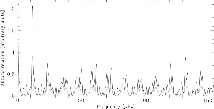
Figure 4: Autocorrelation of the power spectrum with a threshold of 0.07 m² s^-1. The gray line corresponds to the same autocorrelation but all peaks greater than the threshold have the same amplitude (not to favour only the highest peaks). The large spacing is estimated to be about 72 $\mu$Hz.

In solar-like stars, p-mode oscillations of low-degree are expected to produce a characteristic comb-like structure in the power spectrum with mode frequencies $\nu_{n,l}$ reasonably well approximated by the asymptotic relation (?):

$$\nu_{n,l} \approx \Delta\nu(n+\frac{l}{2}+\epsilon)-l(l+1)D_{0}\;.$$ (1)

Here, $D_{0}$, which is equal to $\frac{1}{6}\delta\nu_{02}$ if the asymptotic relation holds exactly, and $\epsilon$ are sensitive to the sound speed near the core and to the surface layers respectively. The quantum numbers $n$ and $l$ correspond to the radial order and the angular degree of the modes, and $\Delta\nu$ and $\delta\nu_{02}$ to the large and small spacings. To fit to this relation, an autocorrelation of the power spectrum is calculated and presented in Fig. 4. The threshold of the power spectrum (all frequencies with a smaller amplitude than this value has its amplitude fixed to zero) is chosen to 0.07 m² s^-1 corresponding to a signal to noise of 3.5 in amplitude, this process can diminish the noise. Each peak of the autocorrelation corresponds to a structure present in the power spectrum. The two strong peaks at low frequency near 11.6 and 23.1 $\mu$Hz correspond to the daily aliases. The strongest other peaks are situated near 60 $\pm$ 11.57 $\mu$Hz and 130 $\pm$ 11.57 $\mu$Hz which correspond respectively to one and two times the large spacing. We can thus deduce that the large spacing is near 72 $\mu$Hz, as peaks at 2 times a separation of 60 or 80 $\mu$Hz are not present, this is in accordance with theoretical predictions (see Sect. 1). Three peaks coexist near 72 $\mu$Hz, namely 70.5, 72 and 74 $\mu$Hz, but the most probable large spacing is situated at 72 $\mu$Hz: a high peak has the value of 2 times this spacing whereas only a low peak is present near 141 $\mu$Hz, and no peak at all near 148 $\mu$Hz. This large spacing will be in any case refined during the following step.

3.4 Mode identification

Table 2: Identification of extracted frequencies. The number of peaks due to noise is in agreement with the simulations described in Sect. 3.4, which predict 4.9 $\pm$ 4.3 noise peaks.

Frequency	Mode ID	S/N
$[\mu$Hz$]$
$720.1+11.6=731.7$	$\ell=1$	3.2
$814.6-11.6=803.0$	$\ell=1$	3.0
$920.9-11.6=909.3$	$\ell=0$	3.3
982.6	$\ell=0$	4.2
$1113.3+11.6=1124.9$	$\ell=0$	4.1
$1165.3-11.6=1153.7$	$\ell=1$	3.8
$1212.6+11.6=1224.2$	$\ell=1$	3.1
1258.7	$\ell=2$	3.3
1266.1	$\ell=0$	4.1
1291.7	noise	4.1
1298.7	$\ell=1$	4.6
$1329.1+11.6=1340.7$	$\ell=0$	3.9
$1382.2-11.6=1370.6$	$\ell=1$	4.6
$1391.8+11.6=1403.2$	$\ell=2$	3.0
$1421.2-11.6=1409.6$	$\ell=0$	6.1
$1430.9+11.6=1442.5$	$\ell=1$	3.9
1447.9	noise	3.3
1478.5	$\ell=2$	4.2
1479.9	$\ell=2$	4.5
$1527.8-11.6=1516.2$	$\ell=1$	4.5
1553.6	$\ell=2$	5.2
$1598.7-11.6=1587.1$	$\ell=1$	3.3
1624.1	$\ell=2$	4.0
1697.8	$\ell=2$	3.0
$1691.1+11.6=1702.7$	$\ell=0$	3.1
$1754.9+11.6=1766.5$	$\ell=2$	3.1
$1818.9-11.6=1807.3$	$\ell=1$	3.9
$1835.0+11.6=1846.6$	$\ell=0$	3.5
1875.2	$\ell=1$	3.6
$2147.0-11.6=2135.4$	$\ell=0$	4.1
2168.4	$\ell=1$	3.2
$2249.8-11.6=2238.2$	$\ell=1$	3.2
$2340.9+11.6=2352.5$	$\ell=0$	3.4

Figure 5: Top: Original power spectrum of $\beta$ Vir. Bottom: Cleaned power spectrum: all peaks listed in Table 2 have been removed. The dot-dashed, dotted and dashed lines indicate an amplitude of 5 $\sigma$, 4 $\sigma$ and 3 $\sigma$, respectively. Numerous peaks are still present below 3 $\sigma$, since no peaks have been cleaned below this threshold. These peaks can be due to $p$–mode oscillations and noise or have artificially been added by the extraction algorithm due to the finite lifetimes of the modes

Figure 6: Power spectrum of $\beta$ Vir with the thirty-one extracted frequencies indicated by dashed lines. The identification of each extracted frequency is given in Table 3.

The frequencies were extracted using an iterative algorithm, which identifies the highest peak between 700 and 2400 $\mu$Hz and subtracts it from the time series. Note that because of the stochastic nature of solar–like oscillations, a timestring of radial velocities cannot be expected to be perfectly reproduced by a sum of sinusoidal terms. Therefore, using an iterative clean algorithm to extract the frequencies can add additional peaks with small amplitudes due to the finite lifetimes of the modes that we do not know. Nevertheless, the iterative algorithm ensures that one peak and its aliases with an amplitude above a given threshold is only extracted once. To avoid extracting artificial peaks with small amplitudes added by the iterative algorithm, the choice of this threshold is important. In the case of $\beta$ Vir, we iterated the process until all peaks with an amplitude higher than 3 $\sigma$ in the amplitude spectrum were removed (see Fig. 5). Peaks with amplitudes below the 3$\sigma$ threshold were not considered since they were too strongly influenced by noise and by interactions between noise and daily aliases. This threshold, which ensures that the selected peaks have only a small chance to be due to noise, gave a total of twenty-three frequencies (see Table 2). Because of the daily alias of 11.57 $\mu$Hz introduced by the monosite observations, we cannot know a priori whether the frequency selected by the algorithm is the right one or an alias. We thus considered that the frequencies could be shifted by $\pm 11.57$ $\mu$Hz, and made echelle diagrams for different large spacings near 72 $\mu$Hz until every frequency could be identified as an $\ell=0$, $\ell=1$ or $\ell=2$ mode. In this way, we found an averaged large spacing of 72.1 $\mu$Hz.

To investigate how many peaks are expected to be due to noise, we have conducted simulations in which we analyzed noise spectra containing no signal. For this purpose, a velocity time series is built, using the observational time sampling and radial velocities randomly drawn by assuming a Gaussian noise (Monte–Carlo simulations). The amplitude spectrum of this series is then calculated and peaks with amplitude greater than 3, 4 and 5 $\sigma$ are counted; note that a peak and its aliases are only counted once. The whole procedure is repeated 1000 times to ensure the stability of the results. In this way, we find that the number of peaks due to noise with an amplitude larger than 3 $\sigma$ is 4.9 $\pm$ 4.3 in the range 0.7–2.4 mHz, for 4 $\sigma$, the number of peaks due to noise varies between 0 and 3 with a mean value of 0.0 and a standard deviation of 0.5. No peaks due to noise are expected with an amplitude larger than 5 $\sigma$.

Table 3: Oscillation frequencies (in $\mu$Hz) of $\beta$ Vir. The frequency resolution of the time series is 1.14 $\mu$Hz.

	$\ell$ = 0	$\ell$ = 1	$\ell$ = 2
n = 8		731.7
n = 9		803.0
n = 10
n = 11	909.3
n = 12	982.6
n = 13
n = 14	1124.9	1153.7
n = 15		1224.2	1258.7
n = 16	1266.1	1298.7
n = 17	1340.7	1370.6	1403.2
n = 18	1409.6	1442.5	1478.5 / 1479.9
n = 19		1516.2	1553.6
n = 20		1587.1	1624.1
n = 21			1697.8
n = 22	1702.7		1766.5
n = 23		1807.3
n = 24	1846.6	1875.2
n = 25
n = 26
n = 27
n = 28	2135.4	2168.4
n = 29		2238.2
n = 30
n = 31	2352.5
$\Delta\nu_{\ell}$	72.18 (0.09)	71.91 (0.15)	72.82 (0.30)

The echelle diagram showing the thirty-one identified modes is shown in Fig. 7. The frequencies of the modes are shown in Fig. 6 and are given in Table 3, with radial order of each oscillation mode deduced from the asymptotic relation (see Eq. 1) assuming that the parameter $\epsilon$ is near the solar value ($\epsilon_{\odot}\sim 1.5$). The average large spacing and the parameters $D_{0}$ and $\epsilon$ are thus deduced from a least-squares fit of this equation with the frequencies of Table 3. The average small spacing is here defined as $D_{0}\times 6$ (the perfect asymptotic case, with constant large and small separations):

$$\Delta\nu_{0}\,=\,72.07\,\pm\,0.10\;\mu Hz,\ \epsilon\,=\,1.59\,\pm\,0.03\;,$$

$$D_{0}\,=\,1.05\,\pm\,0.24\;\mu Hz,\ \langle\delta\nu_{02}\rangle\,=\,6.28\,\pm\,1.42\;\mu Hz.$$

The small spacing appears to decrease from 7.4 to 4.9 $\mu$Hz between 1260 and 1700 $\mu$Hz. $\beta$ Vir has a projected rotational velocity of about $v$ $\sin$ $i$ $\sim$ 4.3 km s^-1 (?). We can estimate its radius to $R$ = 1.66 $R_{\odot}$ from $L$ = 3.51 $L_{\odot}$ (Hipparcos data) and $T_{\rm eff}$ = 6140 ^∘ K (?). Assuming an uniform rotation, we determine the corresponding splitting of the modes to be at least 0.56 $\mu$Hz (for $\sin$ $i$ = 1). This splitting can increase the uncertainty of the mode frequencies. $\ell=1$ modes can thus be shifted by at least $\pm$0.56 $\mu$Hz, this effect is worse on $\ell=2$ modes (twice this value). Indeed, the dispersions of $\ell=2$ and $\ell=1$ modes are greater than for $\ell=0$ modes (see Fig. 7 and Table 3 with the larger errors on $\Delta\nu_{2}$ and $\Delta\nu_{1}$). Moreover, two high $\ell=2$ modes were determined with a same radial order (1478.5 and 1479.9 $\mu$Hz), this could be explained by such a splitting, implying an angle $i$ near 53^∘, however, with a high uncertainty.

Both $\ell=1$ modes at 731.7 and 803.0 $\mu$Hz could be shifted by 11.57 $\mu$Hz. They were fixed to their value in order to follow the slight curvature present for $\ell=0$ modes at low frequency. They have to be taken with some caution.

Figure 7: Echelle diagram of identified modes with a large separation of 72.1 $\mu$Hz. The modes $\ell$=2 ($\blacksquare$), $\ell$=0 ($\bullet$), and $\ell$=1 ($\blacktriangle$) are represented with a size proportional to their amplitude.

3.5 Oscillation amplitudes

Concerning the amplitudes of the modes, theoretical computations predict oscillation amplitudes near 50 cm s^-1 for a 1.25 $M_{\odot}$ star like $\beta$ Vir, with mode lifetimes of the order of several days to several tenth of days. (?). The amplitudes of the highest modes, in the range 32–46 cm s^-1, are then slightly lower than expected. The observations indicate that oscillation amplitudes are typically 1.5–2 times solar. This disagreement can be partly explained by the lifetimes of the modes. Indeed, the oscillation modes have finite lifetimes, because they are continuously damped. Thus, if the star is observed during a time longer than the lifetimes of the modes, the signal is weakened due to the damping of the modes and to their re–excitation with a random phase.

4 Conclusion

The radial velocity measurements of $\beta$ Vir, obtained over 11 nights, show a significant excess in the power spectrum between 0.7–2.4 mHz, centered around 1.4 mHz, with a maximal peak amplitude of 45 cm s^-1, revealing solar–like oscillations. Moreover, we presented the identification of thirty-one individual frequencies. Note that this identification is a little complicated by the presence of rotational splitting, as $\beta$ Vir rotates rapidly enough to see this effect. The signal-to-noise of our data is unfortunately not high enough to unambiguously determine this splitting. The oscillation modes present an average large spacing of 72.1 $\mu$Hz, and the small spacing appears to decrease from 7.4 to 4.9 $\mu$Hz between 1260 and 1700 $\mu$Hz, with an average of 6.3 $\mu$Hz. As the large spacing is related to $\sqrt{M/R^{3}}$ (?), the mass of $\beta$ Vir should be close to 1.3 M_⊙. Detailed theoretical models of $\beta$ Vir will be reported in a subsequent paper.

References

- [1]
- [2] [] Bouchy, F., Carrier, F., 2002. A&A, 390, 205 (2002A&A...390..205B)
- [3] [] Carrier, F., Bourban, G., 2003. A&A, 406, L23 (2003A&A...406L..23C)
- [4] [] Carrier, F., Bouchy, F., Eggenberger, P., 2003. Recent Research Developments in Astronomy & Astrophysics, 1, I, 219, Research Signpost, India, ISBN 81-271-0002-1
- [5] [] Carrier, F., Bouchy, F., Kienzle, F., et al., 2001. A&A, 378, 142 (2001A&A...378..142C)
- [6] [] Connes, P., 1985. Ap&SS, 110, 211 (1985Ap&SS.110..211C)
- [7] [] Glebocki, R., Stawikowski, A., 2000. AcA, 50, 509 (2000AcA....50..509G)
- [8] [] Gray, R.O., Graham, P.W., Hoyt, S.R., 2001. AJ, 121, 2159 (2001AJ....121.2159G)
- [9] [] Houdek, G., Balmforth, N.J., Christensen–Dalsgaard, J., Gough, D.O., 1999. A&A, 351, 582 (1999A&A...351..582H)
- [10] [] Kjeldsen, H., Bedding, T.R., 1995. A&A, 293, 87 (1995A&A...293...87K)
- [11] [] Lomb, N.R., 1976. Ap&SS, 39, 447 (1976Ap&SS..39..447L)
- [12] [] Pepe, F., Mayor, M., Rupprecht, G., et al., 2002. The Messenger, 110, 9 (2002Msngr.110....9P)
- [13] [] Scargle, J.D., 1982. ApJ, 263, 835 (1982ApJ...263..835S)
- [14] [] Tassoul, M., 1980. ApJS, 43, 469 (1980ApJS...43..469T)