The Spectral Variability of Pulsating Stars: PG 1159-035

Abstract

With 10m class telescopes as well as with time-tagging detectors on board of HST and FUSE, the analysis of time-resolved spectra for pulsating white dwarfs becomes feasible. We present simulated time-resolved spectra for the hot pulsating white dwarf PG 1159-035 and compare these models with observational data of the 516 s mode based on HST-STIS spectroscopy. A determination of the pulsation mode by the spectral variability of PG 1159-035 seems to be impossible for the moment.

Institut für Astrophysik, Universität Göttingen, Friedrich-Hund-Platz 1, D-37077 Göttingen, Germany

Institut für Astronomie und Astrophysik, Universität Tübingen, Sand 1, D-72076 Tübingen, Germany

1. Introduction

Analyses of stellar oscillations are important tools for probing stellar structure and evolution and hence for analyses of white dwarfs as well. Variable white dwarfs are non-radial g-mode-pulsators whose pulsation modes can be described in terms of spherical harmonics with parameters $l$ and $m$. PG 1159-035 is the prototype for hot pulsating H-deficient white dwarf stars at the transition stage to the white dwarf sequence. The response of stellar atmospheres to pulsations can be seen in wavelength-dependent flux variations. We calculate these wavelength-dependent flux variations for modes with different $l$ and compare them with observational data based on HST-STIS spectra. The goal is to get an independent method for analyses of pulsation properties and the determination of pulsation modes as a supplement to photometric analyses (e.g. Winget et al. 1991; Kawaler & Bradley 1994).

In this paper, we describe our first approach towards the spectral analysis of the pulsating white dwarf PG 1159-035. We begin in Section 2 with a description of the model properties on which our analysis is based. In Section 3, we present calculations of chromatic amplitudes for different pulsation modes and compare these with observational data in Section 4. We present our conclusions in Section 5.

2. Spectral Analysis of PG 1159-035

Our analysis is based on theoretical spectra which are calculated with a NLTE model atmosphere program (Werner & Dreizler 1999; Dreizler 2003; Werner et al. 2003) using detailed H-He-C-O model atoms (Werner et al. 2004). Our model grid ranges from T_eff=137000-143000 K (in steps of 250 K) for $\log{g}=7.0$ and $\log{g}=6.8-7.2$ (in steps of 0.1 dex) for T_eff=140000 K, respectively. These values are distributed around the parameters T_eff=140000 K and $\log{g}=7.0$ derived in earlier analyses (Werner et al. 1991; Dreizler & Heber 1998).

Figure 1 shows a normalized model spectrum for T_eff=140 kK and $\log{g}=7.0$ as well as flux variations relative to this model caused by variations in temperature and surface gravity, respectively.

Figure 1.: Flux variation relative to the best fit model with T_eff=140 kK and $\log{g}=7.0$. The left plot shows flux variations for several temperatures and fixed $\log{g}=7.0$. The right plot shows flux variations for several values of $\log{g}$ and a fixed temperature of T_eff=140 kK (upper panel) as well as a model of the normalized flux for T_eff=140 kK and $\log{g}=7.0$ (lower panel). All spectra are convolved with a 1.5 Å Gaussian.

3. Chromatic Amplitudes

According to Robinson et al. (1982, 1995) we calculate the wavelength-dependent flux variations between 200 Å and 7000 Å by

$$F_{\lambda} \propto I_{0\lambda}\int{h_{\lambda}(\mu)\;\mu\;d\mu}$$

$$\Delta F_{\lambda} \propto I_{0\lambda}\left(\frac{1}{I_{0\lambda}}\frac{\partial I_{0\lambda}}{\partial T}\right)\int{h_{\lambda}(\mu)\;P_{l}(\mu)\;\mu\;d\mu}$$

where $P_{l}(\mu)$ is the Legendre polynomial of degree $l$ (all models with $m$=0) and the integrals are evaluated between $\mu=0$ and $\mu=1$. We derive a limb darkening $h_{\lambda}$ from nine angle values of $\mu$ between $\mu=0$ and $\mu=1$ for each wavelength in each spectrum and replace the derivative $(\partial I_{0\lambda}/\partial T)$ by a difference quotient $\Delta I_{0\lambda}/\Delta T$ computed with models of $T_{\rm eff}$=139750 K and $T_{\rm eff}$=140250 K for each wavelength.

Figure 2 shows our results of calculated chromatic amplitudes $\Delta F_{\lambda}/F_{\lambda}$ using the best model with parameters T_eff=140000 K, $\log{g}=7.0$ for pulsation modes with $l$=1-3 ($m$=0).

Unfortunately, our models show almost no difference between pulsation modes with $l$=1 and $l$=2 in nearly the whole wavelength range, especially for wavelengths between 1100 Å  and 1800 Å.

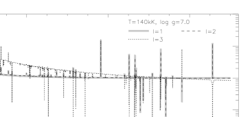
Figure 2.: Chromatic amplitudes $\Delta F_{\lambda}/F_{\lambda}$ calculated for T_eff=140000 K and $\log{g}=7.0$ and for pulsation modes with $l$=1-3 and wavelengths ranging from 200-7000 Å; chromatic amplitudes are normalized at 5500 Å and are convolved with a 1.5 Å Gaussian.

4. Observation

The observational time-resolved spectra of PG 1159-035 were obtained during Cycle 10 with the HST-STIS. The observations were obtained with the G140L grating and a 52x0.2 slit in time-tagged mode. The 20 orbits are grouped into seven blocks of about 40 min exposure time. Afterwards, the 20 orbits are split into 955 blocks of about 50 s during data reduction with IRAF SDSDAS routines. The observed chromatic amplitudes were obtained by binning the spectra by 20 Å  and fitting sine functions with periods fixed to the modes determined from WET observations (Winget et al. 1991). Observed chromatic amplitudes shown in Figure 3 are obtained from the most prominent pulsation mode with a period of P=516.040 s. For comparison, Figure 3 shows our calculated models for pulsation modes with $l$=1-3, as well. Models are normalized at 1700 Å and the observations are normalized at the mean value of chromatic amplitudes for 1660 Å, 1680 Å, and 1700 Å in order to remove systematic deviations between the models and the observational data.

Figure 3 doesn’t allow the determination of the pulsation mode of the 516 s period: although the observation roughly matches the slope of the $l$=1 and $l$=2 mode, the difference between these models are too small and the fluctuation of the observational data around the models is too high for further analyses.

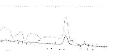
Figure 3.: Chromatic amplitudes as in Figure 2 compared with the 516 s mode of PG 1159-035 obtained from HST-STIS spectroscopy. The models are convolved with a 20 Å Gaussian in order to match the observational binning.

5. Summary and Conclusions

We have calculated the chromatic amplitudes for pulsation modes with $l$=1-3 to analyze the spectral variability of the hot pulsating white dwarf PG 1159-035. Our models show almost no difference between modes with $l$=1 and $l$=2 in the UV and optical wavelength range. For the moment therefore, it seems to be impossible to determine pulsation modes of GW Vir pulsators by their spectral variability.

There are two obvious means of improving our results: we can expand the wavelength range of our observational data to shorter wavelengths, e.g. with FUSE data; and - from a theoretical point of view - we will try to improve our models by surface-resolved flux synthesis.

Acknowledgments.

T. Stahn would like to thank the organizers of the workshop for financial support.

Observations were made with NASA/ESA Hubble Space Telescope, obtained from the data archive at the Space Telescope Institute.

References

- Dreizler (2003) Dreizler, S. 2003, in ASP Conf. Ser. 288: Stellar Atmosphere Modeling, ed. I. Hubeny, D. Mihalas, & K.Werner, 69
- Dreizler & Heber (1998) Dreizler, S. & Heber, U. 1998, A&A, 334, 618
- Kawaler & Bradley (1994) Kawaler, S. D. & Bradley, P. A. 1994, ApJ, 427, 415
- Robinson et al. (1982) Robinson, E. L., Kepler, S. O., & Nather, R. E. 1982, ApJ, 259, 219
- Robinson et al. (1995) Robinson, E. L., Mailloux, T. M., Zhang, E., et al. 1995, ApJ, 438, 908
- Werner & Dreizler (1999) Werner, K. & Dreizler, S. 1999, in Computational Astrophysics, ed. H. Riffert & K. Werner, Journal of Computational and Applied Mathematics, Vol. 109, 65
- Werner et al. (1991) Werner, K., Heber, U., & Hunger, K. 1991, A&A, 244, 437
- Werner et al. (2003) Werner, K., Deetjen, J. L., Dreizler, S., et al. 2003, in ASP Conf. Ser. 288: Stellar Atmosphere Modeling, ed. I. Hubeny, D. Mihalas, & K.Werner, 31
- Werner et al. (2004) Werner, K., Rauch, T., Barstow, M. A., & Kruk, J. W. 2004, A&A, 421, 1169
- Winget et al. (1991) Winget, D. E., Nather, R. E., Clemens, J. C., et al. 1991, ApJ, 378, 326