Coronal properties of G-type stars
in different evolutionary phases

We report on the analysis of XMM-Newton observations of three G-type stars in very different evolutionary phases: the weak-lined T Tauri star HD 283572, the Zero Age Main Sequence star EK Dra and the Hertzsprung-gap giant star 31 Com. They all have high X-ray luminosity ($\sim 10^{31}$ erg s^-1 for HD 283572 and 31 Com and $\sim 10^{30}$ erg s^-1 for EK Dra). We compare the Emission Measure Distributions ($EMD$s) of these active coronal sources, derived from high-resolution XMM-Newton grating spectra, as well as the pattern of elemental abundances vs. First Ionization Potential (FIP). We also perform time-resolved spectroscopy of a flare detected by XMM from EK Dra. We interpret the observed $EMD$s as the result of the emission of ensembles of magnetically confined loop-like structures with different apex temperatures. Our analysis indicates that the coronae of HD 283572 and 31 Com are very similar in terms of dominant coronal magnetic structures, in spite of differences in the evolutionary phase, surface gravity and metallicity. In the case of EK Dra the distribution appears to be slightly flatter than in the previous two cases, although the peak temperature is similar.

1 Introduction

During the last decade, the analysis of high-resolution X-ray spectra of late-type stars, obtained with EUVE, XMM-Newton and Chandra (e.g. Monsignori Fossi et al., 1995; Schmitt et al., 1996; Güdel et al., 1997; Griffiths & Jordan, 1998; Laming & Drake, 1999; Sanz-Forcada et al., 2002; Argiroffi et al., 2003), revealed that the thermal structure of coronal plasmas is better described by a continous Emission Measure Distribution, $EMD$, rather than by the combination of a few isothermal components usually employed to fit low- and medium-resolution spectra. Since the coronal plasma is optically thin, the $EMD$ of the whole stellar corona can be viewed as the sum of the emission measure distributions of all the loop-like structures where the plasma is magnetically confined; therefore, it can be used to derive information about the properties of the coronal structures and the loop populations (Peres et al., 2001). In particular, the studies mentioned above have indicated that the coronae of intermediate and high activity stars appear to be more isothermal than coronae of solar-type stars, and that the bulk of the plasma emission measure is around $\log T\sim 6.6$ for stars of intermediate activity and up to $\log T\sim 7$ for very active stars. The latter result is consistent with the one previously obtained from the analyses of Einstein and ROSAT data, i.e. that there is a good correlation between the effective coronal temperature and the X-ray emission level (see, for example, Schmitt et al., 1990; Preibisch, 1997).

The observation that in active stars a considerable amount of plasma steadily resides at very high temperatures, which are achieved on the Sun only during flaring events, led to the hypothesis that a superposition of unresolved flares may heat the plasma causing an enhanced quasi-quiescent coronal emission level. Following this idea, Güdel (1997) showed that the time-averaged $EMD$ resulting from hydrodynamic simulations of a statistical set of flares, distributed in total energy as a power law, could be made quite similar to the $EMD$ of stars of different activity level (and age). In particular, he obtained distributions with two peaks and a minimum around 10 MK; the amount of the hottest plasma (at $\sim 12-30$ MK) decreases with decreasing $L_{\rm X}$ (or, equivalently, with increasing age) and, at the same time, the first peak moves towards lower temperatures.

A qualitatively different scenario for the evolution of the $EMD$ with activity has been proposed by J. Drake (see Fig. 2 in the review by Bowyer et al., 2000): the distribution increases monotonically from the minimum, which occurs at $\log T$ between $\sim 5$ and $6$, up to the peak at coronal temperatures; the location of the peak shifts towards higher and higher temperatures (up to $\log T\sim 7$ in the most active stars) for increasing X-ray activity level. Along with the shift of the peak, the steepness of the ascending part of the distribution increases.

In the pictures sketched above, the shape of the $EMD$ changes with the stellar activity level; however, it is not yet understood which stellar parameters (luminosity, surface flux, surface gravity, evolutionary phase, or others) have a major role in determining the physical characteristics of the dominant coronal structures and, hence, the properties of the whole Emission Measure Distribution.

In order to investigate this issue, we have examined the cases of three G-type stars, in different evolutionary phases: the Pre-Main Sequence star HD 283572, the Zero-Age Main Sequence star EK Draconis (HD 129333) and the Hertzsprung-gap giant star 31 Com (HD 111812). Here we report on the analyses of recent XMM-Newton observations of these bright targets, characterized by similar and relatively high X-ray luminosities ($L_{\rm X}\sim 10^{30}$ erg s^-1 for EK Dra, and $L_{\rm X}\sim 10^{31}$ erg s^-1 for HD 283572 and 31 Com) with respect to the Sun. Previous analyses (e.g. Güdel et al., 1997; Ayres et al., 1998; Favata et al., 1998) showed that the characteristic coronal temperatures of the stars of our sample lie around $10^{7}$ K; the EPIC and RGS detectors on board XMM are very sensitive to this temperature regime, allowing us to get rather accurate and reliable information about the plasma Emission Measure Distributions of these stars.

The analysis of the XMM observation of 31 Com was reported in Scelsi et al. (2004), while the reconstruction of the $EMD$ of HD 283572 using a high-resolution spectrum is presented here for the first time. For ease of comparison with these two sources, we have also re-analyzed the XMM observation of EK Dra using the same method employed for 31 Com and HD 283572, thus ensuring homogeneity of the results; note however that independent analyses of the same XMM observation of EK Dra have been published since 2002 (e.g. Güdel et al., 2002; Telleschi et al., 2003) and more recently and comprehensively by Telleschi et al. (2004) in the context of a study of solar analogs at different ages. The latter work is complementary to our present study because it considers stars having similar mass, size and gravity, but largely different $L_{\rm X}$ and coronal temperature.

This paper is organized as follows: we describe the three targets in Sect. 2 and we present the observations in Sect. 3. In Sect. 4 we describe the data reduction and the methods used for the analyses of EPIC and RGS spectra. The results are shown in Sect. 5 and discussed in Sect. 6.

2 The sample

In Fig. 1 we plot the positions of the sample stars in the H-R diagram, to show their respective evolutionary phases. We used visual magnitudes, $B-V$ color indexes and distances measured by $Hipparcos$; we assumed negligible optical extinction in the cases of EK Dra and 31 Com, coherent with the low interstellar absorption used in the analysis of their X-ray spectra (Sect. 5), while we used a visual extinction $A_{V}=0.57$ (Strom et al., 1989) and $E_{B-V}\sim A_{V}/3$ for HD 283572.

Figure 1: Positions of HD 283572, EK Dra and 31 Com in the H-R diagram. We have superimposed pre-main-sequence (dashed lines) and post-main-sequence (solid lines) tracks for the mass values reported in the plot. The evolutionary models are those of Ventura et al. (1998a, b), except for the 2 M_⊙ pre-M.S. track, for which we have used the model of Siess et al. (2000). All tracks are calculated for solar photospheric abundances.

Table 1: Stellar parameters. Distances are measured by $Hipparcos$; $L_{\rm x}$ ($0.3-8$ keV) are derived in this work from $3-T$ models; gravities are determined from the corresponding $M$ and $R$, and surface fluxes from the corresponding $L_{\rm X}$ and $R$. In the last column, the references for $L_{\rm bol}$ are indicated in the entries.

	$M/M_{\odot}$	$R/R_{\odot}$	Spectral	$P_{\rm rot}$	$v\sin i$	$d$	$L_{\rm x}$	$g/g_{\odot}$	$F_{\rm x}$	$L_{\rm x}/L_{\rm bol}$
			type	[d]	[Km s-1]	[pc]	[$10^{30}$ erg s-1]		[$10^{6}$ erg s-1 cm-2]
HD 283572	1.8$\,{}^{a}$	2.7$\,{}^{b}$; 4.1$\,{}^{a}$	G2	1.55$\,{}^{a}$	78$\,{}^{a}$	128	$\sim 9$	0.25; 0.12	20; 9	$5\times\,10^{-4}\,{}^{c}$
EK Dra	1.1$\,{}^{d}$	0.95$\,{}^{d}$	G1.5V	2.75$\,{}^{d}$	17.3$\,{}^{e}$	34	$\sim 1$	1.2$\,{}^{f}$	18	$3\times\,10^{-4}\,{}^{g}$
31 Com	3$\,{}^{h}$	9.3$\,{}^{h}$	G0III	$<7.2\,^{i}$	66.5$\,{}^{j}$	94	$\sim 7$	0.035	1.3	$3\times\,10^{-5}\,{}^{h}$
a Strassmeier & Rice (1998a).
b Walter et al. (1987) and the $Hipparcos$ measurement of $d$.
c Walter et al. (1988) and the $Hipparcos$ measurement of $d$.
d Guinan et al. (2003).
e Strassmeier & Rice (1998b).
f Also consistent with the estimate by Strassmeier & Rice (1998b).
g Redfield et al. (2003).
h Pizzolato et al. (2000).
i From $P_{\rm rot}$ and $v\sin i$.
j de Medeiros & Mayor (1999).

The latter star is a member of the Taurus-Auriga star forming region and its age is estimated to be $\sim 2\times 10^{6}$ yr (Walter et al., 1988). HD 283572 shows no sign of accretion from a circumstellar disk, which characterizes the earlier stage of classical T Tauri stars; the decoupling from the disk allowed this star to spin up cosiderably, due to its contraction, up to several tens of km s^-1 ($v\sin i=78$ km s^-1, see Table 1), probably with a consequently enhanced dynamo action and a very high X-ray luminosity ($L_{\rm X}\sim 10^{31}$ erg s^-1). From Fig. 1 we deduce that HD 283572 will be an A-type star during its main sequence phase, and we estimate a mass between $\sim 1.5$ and $\sim 2$ M_⊙, in agreement with the estimate of $1.8\pm 0.2$ M_⊙ by Strassmeier & Rice (1998a). The radius of HD 283572 has been derived by Walter et al. (1987) through the Barnes-Evans relation, $R\sim 3.3$ R_⊙ at an assumed distance of 160 pc, which becomes 2.7 R_⊙ at the new distance of 128 pc measured by $Hipparcos$; more recently, Strassmeier & Rice (1998a) combined photometric measurements, rotational broadening and Doppler imaging technique to determine the radius of HD 283572 in the range $3.1-4.7$ R_⊙, with a best value of 4.1 R_⊙. Due to the uncertainties of these estimates, we decided to consider both of them. We anticipate that our main results are only weakly affected by the choice of one of these values.

EK Dra is a G1.5-type star with mass and radius about equal to the solar values. It has just arrived on the main sequence, thus representing an analog of the young Sun. Because of its age ($\sim 7\times 10^{7}$ yr, Soderblom & Clements, 1987), it suffered little magnetic braking and its short rotational period ($\sim 2.7$ days, Guinan et al., 2003) makes it a bright X-ray source ($L_{\rm X}\sim 10^{30}$ erg s^-1).

The more massive ($M\sim 3$ M_⊙) giant star 31 Com (age $\sim 4\times 10^{8}$ yr, Friel & Boesgaard, 1992) has already evolved out of the main sequence and now it is crossing the Hertzsprung-gap. The position of 31 Com in the H-R diagram and the evolutionary models indicate a spectral type late-B/early-A on the main sequence; therefore, this star has developed a convective subphotospheric layer and a dynamo only in its current post-main sequence evolutionary phase (Pizzolato et al., 2000). The X-ray luminosity is $\sim 7\times 10^{30}$ erg s^-1.

The stellar parameters of the three targets, with the relevant references, are summarized in Table 1. For HD 283572 we report both estimates, mentioned above, of the stellar radius and the corresponding values of gravity and surface X-ray flux.

HD 283572, EK Dra and 31 Com were chosen because their stellar parameters offer the possibility to get useful insight into their coronal properties from the comparison of their $EMD$. Note, in particular, that while the X-ray luminosity of 31 Com and HD 283572 are about equal and larger than that of EK Dra by about an order of magnitude, EK Dra and HD 283572 are the stars with the highest surface fluxes, whose values exceed significantly that of 31 Com, by about one order of magnitude. Note also that the different evolutionary phases imply different stellar internal structures; moreover, these targets have quite different gravities, implying different pressure scale heights and possible changes in the properties of the dominant coronal loops.

Finally, the rapidly rotating stars HD 283572 and 31 Com are putative single sources: this avoids difficulties in the interpretation of the results, due both to the uncertain origin of the emission, in case of multiple components, and to the possibility of an enhanced activity as found, for example, in tidally-locked RS CVn systems. On the contrary, EK Dra has a distant companion (Duquennoy et al., 1991), whose mass is likely between 0.37 M_⊙ and 0.45 M_⊙ (Güdel et al., 1995a). Güdel et al. (1995b) found that the X-ray and radio emissions are modulated with the rotational period, strongly suggesting that the coronal emission comes predominantly from the G star. If we assume that the secondary star has $M\sim 0.4$ M_⊙ and age $\sim 70$ Myr, and has a saturated corona (the worst case), its X-ray luminosity would be $\sim 10^{29}$ erg s^-1, so we might expect contamination of the X-ray emission of the G star from the companion at most at $\sim 10$ % level.

3 Observations

The observations of HD 283572, EK Dra and 31 Com were performed with XMM-Newton respectively on September, 5, 2000 (PI: R. Pallavicini), on December, 30, 2000 (PI: A. Brinkman) and on January 9, 2001 (PI: Ph. Gondoin). The non-dispersive CCD cameras (EPIC MOS and EPIC pn, Turner et al., 2001; Strüder et al., 2001), lying in the focal plane of the X-ray telescopes, have spectral resolution $R=E/\Delta E\sim 5-50$ in the range $0.1-10$ keV, while the two reflection grating spectrometers (RGS, den Herder et al., 2001) provide resolution $R\sim 70-500$ in the wavelength range $5-38$ Å ($0.32-2.5$ keV).

For the present study, we considered only the EPIC pn and RGS data; in Table 2 we report details on the instrument configurations and on the observations.

At the time of these observations, both CCD 7 of RGS1 and CCD 4 of RGS2 were not operating. These CCDs correspond to the spectral regions containing the He–like triplets of neon and oxygen, respectively. Note also that the RGS1 spectrum of HD 283572 is entirely missing, due to instrument setup problems in the early phase of XMM-Newton observations; hence we have no information on the O vii triplet for this source.

Table 2: Log of the XMM-Newton observations.

	Exposure time (ks)			EPIC pn	Q.E. Exposurea (ks)				Count-rateb (s-1)
	pn	RGS1	RGS2	Mode/Filter	pn	RGS1	RGS2		pn	RGS1	RGS2
HD 283572	41.1	0	48.7	Full Frame/Medium	41.1	0	47.4		2.20	0	0.15
EK Dra	46.9	51.7	50.2	Large Window/Thick	38.5	44.9	43.6		2.20	0.16	0.22
31 Com	33.5	41.7	40.5	Full Frame/Thick	32.2	39.6	38.5		1.45	0.11	0.16
a Exposure time for the analysis of the quiescent emission (Q.E.), i.e. excluding the time intervals affected by proton flares,
occurred in the cases of HD 283572 and 31 Com, and by the source flare in the case of EK Dra (see Sect. 4.1).
b Mean count-rate in the $1.2-62$ Å ($0.2-10$ keV) band for pn and in the $5-38$ Å ($0.32-2.5$ keV) band for RGS (1st order
spectrum) relevant to the Q.E. Exposure.

4 Data analysis

We used SAS version 5.3.3, together with the calibration files available at the time of the analysis (June 2002), to reduce the data of HD 283572 and 31 Com; the data of EK Dra were reduced with SAS version 5.4 and the analysis was performed in September 2003. We generated all pn responses with the SAS rmfgen and arfgen tasks.

Good Time Intervals were selected by excluding those time intervals showing the presence of presumable proton flares in the background light curve extracted from CCD 9 of the RGS, following den Herder (2002): we cut the intervals where the count-rate exceeds 0.1 cts s^-1 for 31 Com and 1.6 cts s^-1 in the case of HD 283572 (whose observation is contaminated by high level of background), while we did not exclude any interval in the case of EK Dra.

In order to obtain X-ray light curves and spectra, we extracted the events from a circular region ($\sim 50^{\prime\prime}$ radius) within CCD 4 for HD 283572, while we used annular regions ($\sim 7.5^{\prime\prime}-50^{\prime\prime}$ radii) for 31 Com and EK Dra, because the relevant data were affected by pile-up. In all cases, background photons were extracted from the rest of CCD 4, excluding the sources and their out-of-time events.

4.1 Light curves

Figure 2 shows the pn background-subtracted light curves of the sources, with a 200 s time binning. The light curve of 31 Com is the only one that is consistent with the hypothesis of a constant emission (see Sect. 3.1 in Scelsi et al., 2004).

Figure 2: Background-subtracted pn light curves of HD 283572 (upper), EK Dra (middle) and 31 Com (lower), in the $0.2-10$ keV band and with time bins of 200 s. The vertical lines in the light curve of EK Dra mark the time interval of the flare, excluded from the analysis of the quiescent emission.

In the case of HD 283572, there is evidence of variability of the emission, on a time-scale of the order of 30 ks, which is not a typical flare event. The reduced $\chi^{2}_{\rm r}$ is 5.9 ($229\ d.o.f.$) in the null hypothesis of a constant emission; the variability amplitude, calculated as 0.5 [max(rate)-min(rate)]/mean(rate), is $\sim 20\%$. There is a less pronounced variability on a time-scale of $\sim 10$ ks. From Tables 1 and 2, we note that the duration of the observation is about one third of the stellar rotational period, hence a large fraction of the stellar surface was visible during the pointing; this suggests that at least part of the variability is due to an inhomogeneous distributiuon of active regions over the stellar surface.

The light curve of EK Dra clearly shows the presence of a flare; the vertical lines in the figure mark the start and the end of the flare, obtained as the minimum and maximum times where the hardness-ratio, $HR=(H-S)/(H+S)$, systematically exceeds by more than 1 $\sigma$ the average $HR$ value calculated from time intervals before and after the flare. We excluded the time interval of the flare from the emission measure analysis (Sect. 4.3), since we want to study the thermal properties of the quiescent corona, and we analyzed the flare separately. The quiescent emission of EK Dra is still variable, yielding a reduced $\chi^{2}_{\rm r}=6.2$ ($190\ d.o.f.$) against the null hypothesis of a constant source; the variability is on a time-scale of $\sim 15$ ks and its amplitude (calculated as above) is $\sim 16\%$.

4.2 EPIC pn spectra

Figure 3: EPIC pn spectra of HD 283572, EK Dra and 31 Com with their best-fit model spectra (the parameters of the models are listed in Table 3). The spectra of 31 Com and HD 283572, with their relevant best-fit models, have been shifted by -0.5 and +0.5 dex for clarity.

We have performed global fitting of the EPIC pn spectra (Fig. 3) with the aim of deriving, from multi-component thermal models, the initial guess of the continuum level for the line measurements in the RGS spectra. Moreover, the abundances of some elements (Si, S, Ar, Ca) can be better determined from pn spectra, rather than from RGS spectra, thanks to the wider spectral range of the former – which includes the strong K-shell lines of the relevant H–like and He–like ions – and to the higher photon counting statistics.

We analyzed these spectra with XSPEC v11.2 and we found that an absorbed, optically-thin plasma with three isothermal components provides an acceptable description of each of them (see results in Sect. 5.1). The models are based on the Astrophysical Plasma Emission Database (APED/ATOMDB V1.2) and have variable abundances; we adopted the criterion of leaving free to vary only the abundances of those elements (O, Ne, Mg, Si, S, Fe, Ni, in some cases Ca and Ar) with strong and clearly detectable line complexes in EPIC spectra. The abundances of the other elements were tied to that of iron, their best-fit values being poorly constrained when left free to vary.

We eventually used the high-energy tail of the pn spectrum also to check the high-temperature tail of the emission measure distributions, as described in the next section and in Appendix A.

Finally, we performed time-resolved spectroscopy of the pn data of EK Dra during the flare, to get information on the properties (in particular the size) of the flaring loop, employing the method by Reale et al. (1997). This analysis and its results are reported in Appendix B.

4.3 Emission Measure Reconstruction

The approach we adopted for the line-based analysis of the RGS spectra of each star is discussed in detail in Scelsi et al. (2004) together with a study of its accuracy; here we limit ourselves to report the main points of our iterative method.

We employed the software package PINTofALE (Kashyap & Drake, 2000) and, in part, also XSPEC, and used the APED/ATOMDB V1.2 database which includes the Mazzotta et al. (1998) ionization equilibrium.

We first rebinned and co-added the background-subtracted RGS1 and RGS2 spectra for the identification of the strongest emission lines and the measurement of their fluxes. In this latter step, we adopted a Lorentzian line profile and we assumed initially the continuum level evaluated from the 3-T model best fitting the pn spectrum, because the wide line wings make it impossible to determine the true source continuum below $\sim 17$ Å directly from the RGS data, in particular in the $\sim 10-17$ Å range, where the spectrum is dominated by many strong overlapping lines. Then, with the aim to reconstruct the Emission Measure Distribution ($EMD$) vs. Temperature, we selected a set of lines, among the identified ones, with reliable flux measurements and theoretical emissivities. Most of them are blended with other lines, so the measured spectral feature is actually the sum of the contributions of a number of atomic transitions; accordingly, we evaluated the ”effective emissivity” of each line blend as the sum of the emissivities of the lines which mostly contribute to that spectral feature. Moreover, we carefully selected only iron lines not blended with lines of other elements, because the procedure we employed (see below) uses these iron lines in the first step of the $EMD$ analysis, and estimates of the abundances of the other elements are not yet available at this step.

We performed the $EMD$ reconstruction with the Markov-Chain Monte Carlo (MCMC) method by Kashyap & Drake (1998). This method yields a volume emission measure distribution, $EM(T_{k})=dem(T_{k})\,\Delta\log T$, and related statistical uncertainties $\Delta EM(T_{k})$, where $dem(T)=n_{\rm e}^{2}\,{\rm d}V/{\rm d}\log T$ is the differential emission measure of an optically thin plasma and $\Delta\log T=0.1$ is a constant bin size; the method also provides estimates of element abundances, relative to iron, with their statistical uncertainties. The iron abundance is estimated by scaling the emission measure distribution assuming different metallicities and by comparing the synthetic spectrum with the observed one at $\lambda>20$ Å in the RGS spectrum (this is a spectral region free of strong overlapping emission lines). Finally, we checked the solution obtained with the MCMC by comparing (i) the line fluxes predicted from our solution with the measured ones and (ii) the pn model spectrum, based on the reconstructed $EMD$, with the observed pn spectrum at $E>2$ keV. These checks are illustrated respectively in Fig. 6 and in Appendix A, taking the case of EK Dra as an example (similar results were obtained for the other two stars). In particular, the correct prediction of the O vii-viii line fluxes allowed us to check the reliability of the amount of plasma in the low-temperature tail of the $EMD$; analogously, the correct prediction of the Fe xxiii-xxiv line fluxes and of the high-energy tail of the pn spectrum are important tests for the reliability of the amount of plasma in the high-temperature tail of the $EMD$.

We also checked the consistency between the continuum level assumed for flux measurements and the continuum predicted by the $EMD$. In fact, since our method is iterative, the continuum assumed for flux measurements in the RGS range is adjusted at each iteration for consistency with the $EMD$, and it may become different from that predicted by the $3-T$ model best-fitting the pn spectrum, which is adopted as initial guess. Therefore, this procedure ensures that possible cross-calibration offsets between pn and RGS do not affect the final $EMD$.

5 Results

5.1 3-T models

Table 3: Best-fit models of the EPIC pn data (in the $0.3-8$ keV band), with 90% statistical confidence ranges computed for one interesting parameter at a time; nominal errors on $T_{i}$ and $EM_{i}$ are at the 10% level. Element abundances are relative to the solar ones (Grevesse et al., 1992). Mean temperatures are calculated as $<T>=\sum_{i=1}^{3}EM_{i}\,T_{i}/\sum_{i=1}^{3}EM_{i}$. Abundances and hydrogen column densities without errors were fixed as explained in the text.

	HD 283572	EK Dra	31 Com
$\log T_{1,2,3}\,({\rm K})$	6.64, 7.04, 7.43	6.58, 6.94, 7.33	6.44, 6.92, 7.28
$\log EM_{1,2,3}\,({\rm cm}^{-3})$	53.5, 53.5, 53.7	52.5, 52.4, 52.3	52.6, 53.1, 53.0
$\log<T>\,({\rm K})$	7.21	6.99	7.06
C	0.37	0.57	0.38
N	0.37	0.42	1.54
O	$0.236\,\pm\,0.014$	$0.346\,\pm\,0.015$	$0.58\,\pm\,0.03$
Ne	$0.46\,\pm\,0.03$	$0.83\,\pm\,0.04$	$2.35\,\pm\,0.14$
Mg	$0.32\,\pm\,0.05$	$0.86\,\pm\,0.06$	$1.95\,\pm\,0.13$
Si	$0.25\,\pm\,0.04$	$0.59\,\pm\,0.06$	$1.23\,\pm\,0.11$
S	$0.26\,\pm\,0.09$	$0.15\,\pm\,0.10$	$0.58\,\pm\,0.20$
Ar	0.37	$0.82\,\pm\,0.22$	1.54
Ca	$1.8\,\pm\,0.3$	0.83	1.54
Fe	$0.37\,\pm\,0.01$	$0.83\,\pm\,0.01$	$1.54\,\pm\,0.02$
Ni	$1.52\,\pm\,0.11$	$1.80\,\pm\,0.20$	$4.1\,\pm\,0.3$
$N_{\rm H}\,({\rm cm}^{-2})$	$(8.7\,\pm\,0.4)\times 10^{20}$	$3\times 10^{18}$	$10^{18}$
$\chi^{2}_{\nu}/{\rm d.o.f.}$	1.1/688	1.26/411	1.1/367

Figure 4: Co-added RGS spectra of HD 283572 (upper), EK Dra (middle) and 31 Com (lower) with the identification of the most prominent lines; the bin size is 0.02 Å.

Figure 3 shows the pn spectra with their relevant 3-T models, obtained by fitting the data in the $0.3-8$ keV range. The best-fit parameters of the models are listed in Table 3.

The presence of the Fe xxv 6.7 keV emission line in all these spectra is indicative of hot coronae, as expected from earlier works and confirmed by our analysis. Note the large best-fit EM values of the hottest components for all stars, comparable to the EMs of the cooler components; in particular, the hottest plasma dominates the corona of HD 283572, as also confirmed by the analysis of $Chandra$ spectra (Audard et al., 2004).

The line complexes of Mg xi-xii ($\sim 1.3-1.5$ keV), Si xiii-xiv ($\sim 1.8-2.1$ keV) and S xv ($\sim 2.5$ keV), as well as the large bump between 0.6 and 1 keV due to the Fe xvii-xxiv, Ni xix-xx and Ne ix-x lines allowed us to constrain the abundances of Mg, Si, S, Fe, Ne and Ni. These complexes are less evident in the spectrum of HD 283572, as a consequence of the significantly lower metallicity with respect to the other two stars; instead, the Ca xix line complex ($\sim 3.9$ keV) is most prominent in the spectrum of this star (Fig. 3) and the estimated abundance of this element is higher than for the other two cases. Note also that we were able to constrain the Ar abundance for EK Dra, thanks to the clearly visible lines of Ar xvii at $\sim 3.1$ keV. In the other two cases we linked the abundances of Ca and/or Ar to that of Fe assuming the same ratios as in the solar corona (Grevesse et al., 1992). Moreover, we used the results of the $EMD$ analyses to fix the coronal C/Fe abundance ratio for EK Dra and 31 Com to respectively 0.7 and 0.25 solar, and the N/Fe ratio for EK Dra to 0.5 solar.

Finally, we could not constrain the interstellar absorption in the directions of EK Dra and 31 Com with the fitting procedure, so we fixed them at the relatively low values of $3\times 10^{18}$ cm^-2 and $10^{18}$ cm^-2 measured, respectively, by Güdel et al. (1997) and Piskunov et al. (1997). On the contrary, the spectrum of HD 283572 is significantly absorbed, as expected from the location of this star in the Taurus-Auriga star forming region. The hydrogen column density we derived from the fit is compatible with $A_{V}$ and consistent with previous results obtained by fitting ASCA, ROSAT, $Einstein$ and SAX data (Favata et al., 1998).

5.2 Emission Measure Distributions and abundances

The rebinned and co-added RGS spectra (Fig. 4) show emission lines from Fe xvii-xxiv, Ne ix-x, O viii and Ni xix-xx ions in all cases, while O vii, Mg xi-xii and Si xiii-xiv emission lines are visible only for EK Dra and 31 Com, and the N vii line in the case of EK Dra only. Actually, we could not identify any line outside the wavelength range $10-20$ Å in the spectrum of HD 283572, because of contamination from high background and lack of the RGS1 spectrum altogether. The reconstruction of the $EMD$ of EK Dra and 31 Com was based on about 40 lines, while we used 25 lines in the case of HD 283572 as a consequence of the lower quality of its spectrum.

Figure 5: Distributions of emission measure derived from RGS data. Values without error bars are not statistically constrained by the MCMC algorithm. Note the different ordinate scale in the plot of EK Dra with respect to those of HD 283572 and 31 Com.

The derived $EMD$s are plotted in Fig. 5; note that the algorithm we used is not able to constrain statistically the values of the emission measure in all the temperature bins. We show in Fig. 6 the observed-to-predicted fluxes for the case of EK Dra, which is representative of the spread of these ratios obtained in our analyses, and in Fig. 7 we compare the observed spectra and the model spectra generated with the solutions ($EMD$ and abundances) found in this work. The elemental abundances are shown in Table 4; we estimated the iron abundances (relative to the solar value) of HD 283572, EK Dra and 31 Com at $0.7\pm 0.2$, $1.2\pm 0.2$ and $1.4\pm 0.2$, respectively. Table 5 reports the ratios $R=f/i$ and $G=(f+i)/r$ relative to the O vii triplet, and the estimates of electron temperatures, densities and pressures, averaged over the region where the triplet forms, using the theoretical curves by Smith et al. (2001).

In Fig. 8 we show the element-to-iron abundance ratios for the three stars, ordering the elements for increasing First Ionization Potential (FIP). Whenever both EPIC pn- and RGS-based estimates were available, we always report the latter in the plot, because we consider the values derived with the RGS the most accurate. It is worth noting that, despite widely differing methods employed to derive elemental abundances, we obtained consistency between the pn- and RGS-derived abundance ratios, except for Ne in the case of 31 Com (the value indicated by the pn is two times larger than the RGS one) and for Ni in the case of EK Dra and HD 283572 (the values obtained with the pn are larger than the RGS ones by factors of 2 and 4 respectively).

Figure 6: Comparison between observed fluxes and the fluxes predicted with the $EMD$ model, for lines used in the EM reconstruction of EK Dra; Fe: open diamonds, Ne: triangles, Mg: open squares, Si: filled diamond, Ni: filled circle, O: filled squares, N: asterisk, C: open circle.

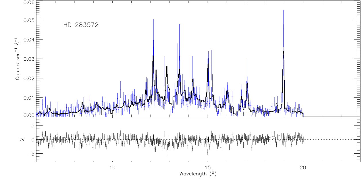
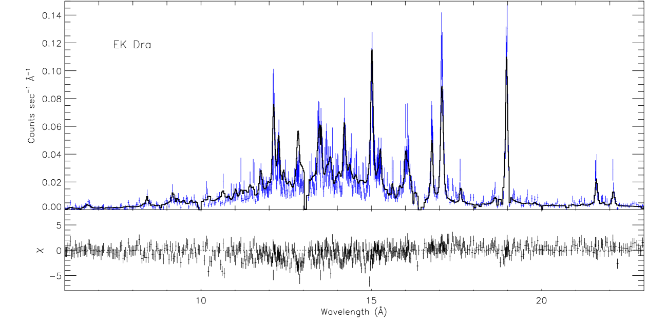
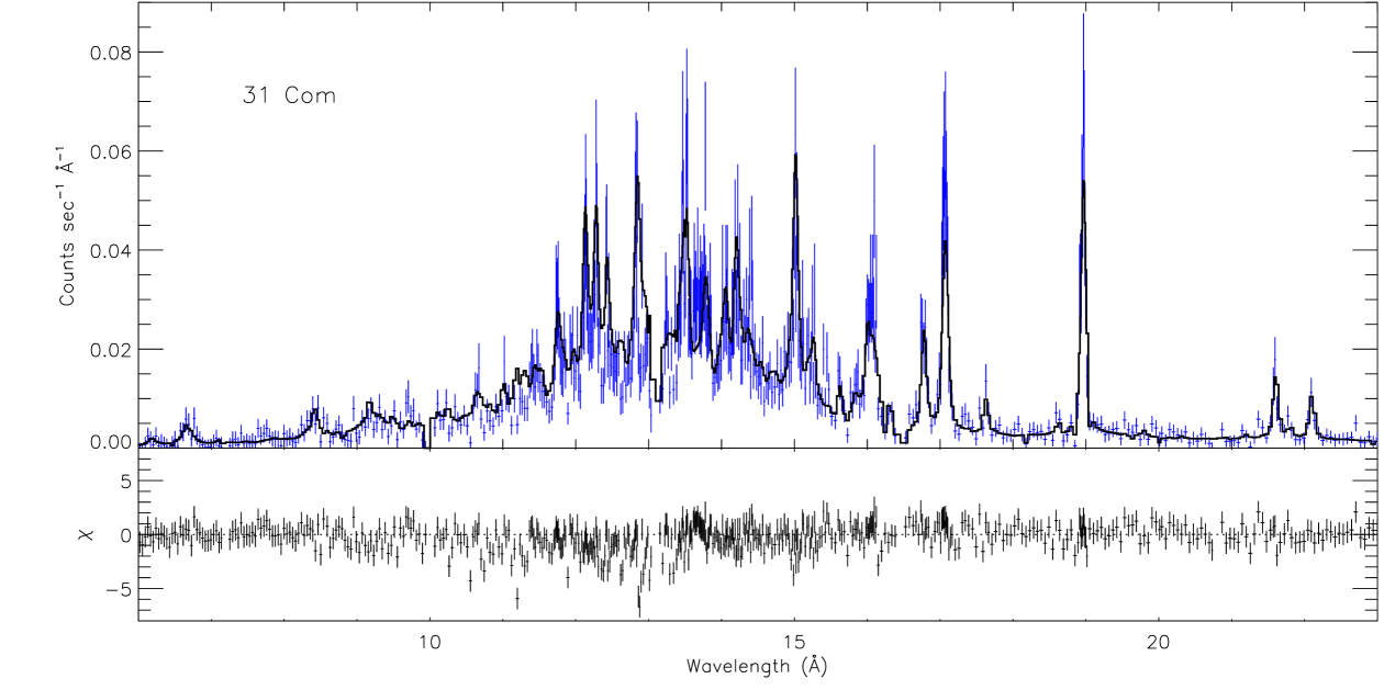
Figure 7: Model spectra compared to the original RGS spectra.

Table 4: Ratios between elemental and iron coronal abundances, relative to the solar photospheric ratios (Grevesse et al., 1992), derived from RGS data; errors are at 68% confidence level. For completeness, we also report the absolute iron abundance. The pn-derived values are shown for purpose of comparison. For each star, the number of lines used for the $EMD$ reconstruction is reported (the number of lines of a given element is shown in parenthesis near the relevant (RGS) abundance value).

	HD 283572		EK Dra		31 Com
	RGS	pn	RGS	pn	RGS	pn
C/Fe			$0.69_{-0.08}^{+0.28}$ (1)		$0.24_{-0.07}^{+0.22}$ (1)
N/Fe			$0.52_{-0.16}^{+0.4}$ (1)
O/Fe	$0.6_{-0.2}^{+0.4}$ (2)	$0.64\,\pm\,0.04$	$0.50_{-0.07}^{+0.04}$ (3)	$0.42\,\pm\,0.02$	$0.49_{-0.08}^{+0.15}$ (2)	$0.38\,\pm\,0.02$
Ne/Fe	$1.2_{-0.3}^{+0.23}$ (2)	$1.24\,\pm\,0.09$	$1.00_{-0.23}^{+0.21}$ (3)	$1.00\,\pm\,0.05$	$0.78_{-0.3}^{+0.13}$ (2)	$1.53\,\pm\,0.09$
Mg/Fe		$0.86\,\pm\,0.14$	$0.88_{-0.13}^{+0.6}$ (2)	$1.04\,\pm\,0.07$	$1.0_{-0.3}^{+0.4}$ (2)	$1.27\,\pm\,0.08$
Si/Fe		$0.68\,\pm\,0.11$	$0.7_{-0.4}^{+0.5}$ (1)	$0.71\,\pm\,0.07$	$0.9_{-0.3}^{+0.9}$ (1)	$0.80\,\pm\,0.07$
Ni/Fe	$1.2_{-0.6}^{+1.0}$ (2)	$4.1\,\pm\,0.3$	$0.9_{-0.3}^{+1.0}$ (1)	$2.17\,\pm\,0.24$	$3.5_{-0.7}^{+2.1}$ (6)	$2.7\,\pm\,0.2$
Fe	$0.7\,\pm\,0.2$ (19)	$0.37\,\pm\,0.01$	$1.2\,\pm\,0.2$ (24)	$0.83\,\pm\,0.01$	$1.4\,\pm\,0.2$ (27)	$1.54\,\pm\,0.02$
total lines	25		36		41

Figure 8: Element-to-iron abundance ratios, relative to the solar photospheric values (Grevesse et al., 1992), for HD 283572 (squares), EK Dra (triangles) and 31 Com (diamonds). The elements are ordered by increasing FIP.

The patterns of abundances vs. FIP are similar in the cases of 31 Com and HD 283572, with an initial decrease (with respect to solar photospheric values) down to a minimum around carbon, followed by increasing abundances for elements with higher FIP ($>11$ eV). This pattern is also similar to what was found for the young active star AB Dor by Sanz-Forcada et al. (2003), but it is less evident in the case of EK Dra. Note that 31 Com and EK Dra have iron abundances differing from that of HD 283572 by about a factor of 2, hence the pattern of abundances vs. FIP appears to be almost independent of the global coronal metallicity.

Table 5: Pressure estimates with O vii.

	$R$	$n_{e}$ (range)	$G$	$T$	$P$ (range)
		($10^{10}$ cm-3)		($10^{6}$ K)	(dyn cm-2)
EK Dra	$3.0\pm 1.7$	$1$ ($<7$)	$0.93\pm 0.25$	$1.5^{+2.0}_{-0.5}$	4 ($<70$)
31 Com	$2.0\pm 1.4$	$3$ ($0.6-20$)	$0.94\pm 0.36$	$1.5^{+2.5}_{-0.7}$	13 ($1.5-220$)

6 Discussion

XMM-Newton data allowed us to derive the plasma emission measure distributions for our three targets and their coronal elemental abundances; in particular, the $EMD$ of HD 283572 has been derived here for the first time using a high-resolution spectrum. Our results are sufficiently well determined and homogeneous for the purpose of a detailed comparison of the coronal properties of the selected stars. We recall that these stars are in different evolutionary stages, but share the characteristic of being active (high X-ray luminosity) G-type stars. Our analysis has confirmed that the three stars have very hot coronae, with similar average temperatures ($\sim 11-12$ MK for EK Dra and 31 Com, and $\sim 16$ MK for HD 283572).

A remarkable result of this work is the close similarity of the emission measure distributions of HD 283572 and 31 Com, which have similar $L_{\rm X}$ as well. Both distributions have a well-defined peak at $T_{\rm p}=10^{7}$ K and, in the range $\log T\sim 6.5-7$, they are proportional to $\sim T^{5}$, where the exponent of the power law has a formal confidence interval between $\sim 3.4$ and $\sim 6.6$; there are also indications of a significant amount of plasma at temperatures hotter than $T_{\rm p}$ (up to $\log T\sim 7.6$) and, at least in the case of 31 Com, in the range $\log T\sim 6-6.2$. We recall that we are not able to statistically constrain the emission measure in all the temperature bins, and hence to get information on the exact shape of the distributions below $\log T\sim 6.5$ and above $\log T\sim 7.3$, yet the presence in both stars of a non-negligible amount of plasma up to $\log T\sim 7.6$ has been verified, as described in Sect. 4.3, through the correct prediction of the Fe xxiii-xxiv line fluxes and by comparison with the high-energy tail of the observed EPIC spectra (App. A), while the correct prediction of the O vii-viii lines allowed us to verify the presence of cool plasma down to $\log T\sim 6$ in the $EMD$ of 31 Com (the O vii line is not available in the spectrum of HD 283572). Note, also, that the shape of the constrained part of the distribution of 31 Com and the presence of significant emission measure at $\log T\sim 6-6.2$ suggest that a minimum in the $EMD$ of this star occurs around $\log T\sim 6.4-6.5$, while some caution is needed for the case of HD 283572.

The $EMD$ of EK Dra is, on average, about one order of magnitude lower than the two previous ones. The distribution has a maximum at $\log T=6.9$, with a more gradual decrease towards higher $T$ than in the two previous cases. Using ASCA/EUVE data, Güdel et al. (1997) derived for EK Dra an $EMD$ essentially bimodal, with two significant peaks near 7 MK and 18 MK. While we also find little plasma at temperatures below $\sim 3$ MK and our value of $T_{\rm p}$ ($\sim 8$ MK) is roughly consistent with their first peak, we do not find either a deep minimum around 10 MK or strong evidence for a second maximum at 18 MK.

It is not straightforward to derive a low-$T$ slope for this distribution, essentially due to the secondary peak at $\log T=6.5$. If we exclude this temperature bin, on the grounds that it belongs to a cooler population of coronal structures (see below), a fitting in the range $\log T=6.6-6.9$, yields a slope of $5.3\pm 1.7$: this is compatible, within errors, with the slopes derived for HD 283572 and 31 Com. Instead, if we consider the secondary peak as a fluctuation produced by the emission measure analysis, the slope in the range $\log T=6.5-6.9$ turns out to be $3.0\pm 1.2$. To address the issue of the $EMD$ slope, we have investigated if a solution smoother than the one presented in Fig. 5 can give a good description of the observed line fluxes as well. Assuming a distribution with its ascending part ($\log T<6.9$) proportional to $T^{3}$ and with the high-temperature tail ($\log T>6.9$) decreasing as $T^{-\beta}$, we searched for the minimum $\chi^{2}$ on the subset of the iron lines, by varing the exponent $\beta$ and a global renormalization factor. The minimum $\chi^{2}$ is obtained for $\beta=1.3$ (the relevant $EMD$ is shown in Fig. 9 together with the reconstructed one), and the observed fluxes for all the selected lines are quite acceptably reproduced (Fig. 10, to be compared with Fig. 6). Note also that we used, for this test, the relative element abundances reported in Table 4. However this solution over-predicts the O viii 18.97 Å/O vii 21.60 Å line ratio: while the observed ratio of line counts is $R_{\rm O,obs}=10.0\pm 1.7$ (1 $\sigma$ error), the ratio predicted by the smooth solution is $R_{\rm O}\sim 16$, against $R_{\rm O}=10.6$ predicted by the MCMC solution. This line ratio does not depend on the oxygen abundance, but it is especially sensitive to the shape of the distribution at low temperatures ($\log T<6.8$), hence its predicted value could be lowered by a small enhancement of the emission measure at $\log T=6.0-6.3$ without affecting significantly the fluxes of the iron lines. Interestingly, our smooth solution is similar to that found recently by Telleschi et al. (2004) using the same XMM data, but a different inversion method. Thus, we are not able to get strong constraints on the low-$T$ slope of the $EMD$ of EK Dra and further investigation is needed.

Figure 9: Emission measure distribution of EK Dra reconstructed in this work using RGS data and the MCMC algorithm (solid line) and the smoothed solution whose shape is proportional to $T^{3}$ for $T<10^{7}$ K and to $T^{-1.3}$ for $T>10^{7}$ K (dashed line).

Figure 10: Comparison between observed fluxes and the fluxes predicted with the smoothed $EMD$ (dashed line in Fig. 9), for lines used in the EMD analysis of EK Dra; Fe: open diamonds, Ne: triangles, Mg: open squares, Si: filled diamond, Ni: filled circle, O: filled squares, N: asterisk, C: open circle.

We want to interpret the shape of the bulk of the emission measure distributions, around $10^{7}$ K, in terms of loop structures. First, we note that, at this high coronal temperature, the pressure scale height $H_{\rm p}$ in each of the three stars is of the order of the corresponding radius (Table 6). We assume that the structures responsible for the observed emission of each star have characteristic sizes smaller than the relevant pressure scale height. In fact, for 31 Com we showed in Scelsi et al. (2004) that loop heigths larger than the stellar radius would be hardly compatible with the absence of variability in the emission of this star, because of the very low filling factor implied by this solution; in Appendix B we analyze the flare on EK Dra and conclude that the height of the flaring loop, which likely belongs to the family of structures dominating the X-ray emission, is a few $10^{10}$ cm; finally, Favata et al. (2001) analyzed a flare on HD 283572 and showed that the size of the involved structure is $\sim 0.3\,R_{*}$. Under this hypothesis, the pressure is approximately uniform inside each loop, implying that the emission measure distribution of a single loop depends only on its maximum temperature $T_{\rm max}$ (Maggio & Peres, 1996), with a functional form $EM(T)\propto T^{\alpha}$ for $T<T_{\rm max}$, with $\alpha=3/2$ in the case of loops with constant cross-section and uniform heating. Considering that the $EMD$ of the whole stellar corona is the sum of the $EM(T)$ of individual loops, the total $EMD$ would be proportional to $T^{\alpha}$ for $T<{\rm min}\{T_{\rm max}\}$; hence, following the approach by Peres et al. (2001), we interpret the constrained part of the $EMD$s of HD 283572 and 31 Com as due to a population of loops, each of them having $EM(T)\propto T^{5}$, since the $EMD$s of these stars are approximatively power-laws (with exponent $\sim 5$) in the temperature range mentioned above. Consequently, the simplest interpretation we derive from the comparison of the emission measure distributions of HD 283572 and 31 Com (Fig. 5, see also Fig. 11 below) is that the coronae of these stars are very similar in terms of dominant coronal structures, in spite of their different evolutionary phases and gravities, as well as coronal abundances. Since this latter parameter plays an important role in the energy balance through the radiative losses, we might expect that different abundances result in different temperature and density profiles along a loop, and hence in different coronal $EMD$s; however, this is not the case in these two stars. Moreover, we stress that HD 283572 and 31 Com show similar $EMD$s in spite of the difference in X-ray surface flux by about one order of magnitude. In conclusion, we infer that all the above parameters have only a minor role in determining the properties of the $EMD$ of these stars, which instead appear to be mainly determined by the high and nearly identical X-ray luminosity.

The high index ($\sim 5$) of the power law which best approximates the ascending part of the $EMD$s of these stars also suggests that the dominant coronal loops of very bright sources (with $L_{\rm X}\sim 10^{31}$ erg s^-1) may have different properties to the solar ones. In such stars, the physical processes that lead to emission measure distributions significantly steeper than those observed in low-luminosity stars, such as the Sun or $\alpha$ Cen (Drake et al., 1997), still remain to be understood; as discussed in Scelsi et al. (2004), a possible interpretation of such steep slopes, which should also characterize the $EM(T)$ of the single structures (see above), is that the heating of the coronal loops is located mainly at their footpoints (Testa & Peres, 2003; Testa et al., 2004). Another possibility are expanding loops, although quite extreme expansion factors are needed (Schrijver et al., 1989); also, both effects might be at work.

The interpretation of the $EMD$ of EK Dra is more uncertain. If we assume that the distribution reconstructed in this work and shown in Fig. 5 is a good approximation of the actual $EMD$ of this star, then a family of hot loops with $EM(T)\propto T^{5}$ appears to be responsible for the bulk of the distribution around $10^{7}$ K, while the emission measure at $\log T<6.6$ may be due to a cooler family of loops whose properties we are not able to investigate with the available data, because of the limited information on the low-temperature plasma; otherwise, if a smoother distribution applies ($EMD\propto T^{3}$, Fig. 9), the structures dominating this corona might have a less steep profile of the emission measure vs. temperature with respect to the cases of HD 283572 and 31 Com, yet steeper than the $T^{3/2}$ slope characterizing uniformly-heated loops with constant cross-section.

Table 6: Stellar radii and pressure scale heigths calculated for $T\sim 10^{7}$ K.

	$R$	$H_{\rm p}$
	(cm)	(cm)
HD 283572	$\sim 3\times 10^{11}$	$\sim 3\times 10^{11}$
EK Dra	$6.6\times 10^{10}$	$4\times 10^{10}$
31 Com	$6.5\times 10^{11}$	$10^{12}$

In Fig. 11, the $EMD$s of the three studied stars are shown together with the emission measure distribution of the Sun (Peres et al., 2000) and $ξ$ Bootis (Laming & Drake, 1999), the latter being a G-type star of intermediate activity, with $L_{\rm X}\sim 10^{29}$ erg s^-1. While the $EMD$ of the Sun peaks at $T_{\rm p}\sim 10^{6.2}$ K, with an ascending part ($\log T\sim 5.7-6.2$) proportional to $T^{3/2}$, and shows no significant amount of plasma at temperatures above $\sim 10^{6.7}$ K, the $EMD$ of $\xi$ Bootis is intermediate between those of the Sun and our active stars, in terms both of $T_{\rm p}$ and of the overall amount of emitting plasma, as well as with regard to the steepness of the $EMD$ preceding its peak. Actually, $\xi$ Bootis is a double star (G8+K4V), but the X-ray emission is thought to be dominated by the primary G8 (Schmitt, 1997), and we have included it in this picture because it is one of the very few stars of intermediate activity whose $EMD$ has been reconstructed from high-resolution spectra.

Figure 11: Emission measure distributions of the coronal plasma of the quiet Sun (Peres et al., 2000, from $Yohkoh$/SXT data), $\xi$ Bootis (Laming & Drake, 1999, from ASCA/EUVE data), EK Dra, 31 Com and HD 283572 (this work). For each of the three active stars, only the constrained part of the $EMD$ is shown.

The comparison shown in Fig. 11 between the $EMD$s of stars with increasing luminosity, going from the quiet Sun to HD 283572, suggests a transition in the steepness of the distribution, which, in turn, may reflect changes of the properties of the dominant coronal loops. Fig. 11 is in agreement with the hypothesis of increasing steepness with increasing $L_{\rm X}$ reported in Bowyer et al. (2000); on the other hand, their picture is not reflected completely by our results which do not indicate, at coronal temperatures, a monotonic increase of the $EMD$ up to its peak, at least in the cases of the bright star 31 Com and possibly also of HD 283572; in fact, the XMM data available for these two stars suggest the presence of plasma at $T\sim 10^{6}$ K and a minimum of the $EMD$ around $T\sim 10^{6.5}$ K.

Finally, it is important to note that the sample is still limited, and new observations are required to have a more complete scenario, as well as to study in greater detail the ”cool” and ”hot” tails of the emission measure distributions of very active stars. In this respect, the recent work by Telleschi et al. (2004) provides complementary results which may help to bridge the gap between solar-type stars and stars with very high activity levels.

Appendix A Checking the high temperature tail of the $EMD$s

As stated at the end of Sect. 4.3, we checked the reliability of the hot tails of the $EMD$s, not constrained by the MCMC method, by comparing the model spectrum with the high-energy ($E>2$ keV) pn spectrum, which is more sensitive to very hot plasma (it contains, in particular, the complex around 6.7 keV largely dominated by Fe xxv and several spectral regions dominated by the bremsstrahlung continuum). This comparison is shown in Fig. 12 for the case of EK Dra, similar results have been obtained for HD 283572 and 31 Com. In this plot, the solid line is the pn model spectrum derived from the reconstructed $EMD$, whose hottest part is reported (with the solid line) in the inset. In the high-energy tail of the spectrum ($2-8$ keV) the model fits well the data ($\chi^{2}_{\nu}\sim 0.98$, 88 $d.o.f.$), indicating reliability of the presence of a sizeable amount of plasma in the high-temperature tail of the $EMD$. We have also examined both the cases of a flatter hot tail with a total emission measure twice as large as the previous case (approximatively proportional to $T^{-3/2}$, shown by the dashed line in the inset), and of a tail which decreases as $T^{-6}$ (dotted line), with a total emission measure four-fold lower than the first case. The corresponding model spectra give a poor fit to the data ($\chi^{2}_{\nu}\sim 4$ and 1.4, respectively, consider that $P(\chi^{2}_{\nu}>1.4)\sim 0.8\%$).

Figure 12: EPIC pn spectrum of EK Dra (crosses) and the model spectrum derived from the reconstructed $EMD$ (solid line); the dashed line is the model spectrum obtained in the case of a distribution equal to the reconstructed one up to $\log T=7.3$, but with a flatter hot tail drawn with the dashed line in the inset; the model spectrum shown with the dotted line, instead, is relevant to a steeper decrease of the hot tail.

Appendix B Analysis of the flare on EK Dra

The flare observed on EK Dra (Fig. 2) has a duration of $\sim 10$ ks and is characterized by a rather wide ($\sim 3$ ks) peak at $\sim 2$ cts/s, subtracting the mean count rate of the quiescent phase, and a secondary maximum at $\sim 0.5$ cts/s which follows the initial decay phase. For the analysis of this flare, we performed time-resolved spectroscopy of the EPIC pn data and employed the approach by Reale et al. (1997) to derive the size of the flaring loop, assuming that the impulsively heated plasma was confined in a single structure. We refer to that paper for a detailed explanation of this method, and to Reale et al. (2004) for its application to a flare (on Proxima Centauri) observed by XMM-Newton.

Table 7: Best-fit values of temperature, emission measure and metallicity (with 90% confidence errors) relevant to the thermal component of the model describing the flaring plasma; for each segment, the (approximated) number of counts in the pn spectrum is also reported.

		variable $z$				fixed $z$
Segment	counts	$T_{\rm obs}$	$EM$	$z$		$T_{\rm obs}$	$EM$
		($10^{7}$ K)	($10^{52}$ cm-3)			($10^{7}$ K)	($10^{52}$ cm-3)
r	3600	$4.2^{+1.6}_{-1.0}$	$4.6^{+1.6}_{-1.5}$	$1(<2.9)$		$4.2^{+1.3}_{-0.9}$	$4.9^{+0.3}_{-0.6}$
p1	4800	$3.3^{+0.7}_{-0.6}$	$9.3^{+1.9}_{-1.8}$	$0.5^{+0.7}_{-0.4}$		$3.4^{+0.5}_{-0.4}$	$8.5^{+0.6}_{-0.5}$
p2${}^{\,{\bf a}}$	4700	$1.86^{+0.4}_{-0.25}$	$10.0^{+1.9}_{-1.8}$	$0.30^{+0.26}_{-0.17}$		$2.2^{+0.25}_{-0.3}$	$7.4^{+0.6}_{-0.5}$
d1	4000	$1.43^{+1.6}_{-0.23}$	$6.5^{+1.9}_{-1.7}$	$0.27^{+0.27}_{-0.15}$		$1.68^{+0.20}_{-0.25}$	$4.2^{+0.4}_{-0.7}$
d2	4100	$1.8^{+0.5}_{-0.3}$	$3.1\pm 0.5$	$0.27^{\,{\bf b}}$		$2.0^{+0.6}_{-0.3}$	$2.1^{+0.4}_{-0.4}$
p3	4800	$2.4^{+1.4}_{-0.8}$	$2.4^{+1.1}_{-1.3}$	$0.48(<2.8)$		$2.5^{+1.1}_{-0.6}$	$2.0^{+0.3}_{-0.3}$
a The agreement between data and model in the case of fixed $z$ is not good ($P(\chi>\chi_{\rm obs})=0.6\%$).
b Fixed to the value of segment d1.

Figure 13: The upper panel shows the light curve of the flare on EK Dra, in the $0.3-10$ keV band of the EPIC pn, obtained by subtracting the average quiescent emission from the total light curve in Fig. 2. The vertical lines mark the phases of the flare. The middle and the lower panels show the time evolution of the temperature and the emission measure, respectively. Filled symbols are relevant to the model with variable global metallicity, open symbols to the model with $z=0.83$ solar.

We divided the observation during the flare into 6 segments (Fig. 13), so as to have $\sim 4000-5000$ counts in the pn spectrum of each of them. These spectra were fitted in XSPEC using, as a model, the fixed 3-T model in Table 3, describing the quiescent emission, plus a fourth component, which gives the temperature and the emission measure of the flaring plasma. We made the fittings both using a variable global metallicity ($z$) and fixing it to the quiescent value ($z=0.83$ solar). The results of the fittings are reported in Table 7 and the evolutions with time of the temperature and the emission measure are shown in the middle and lower panels of Fig. 13.

Unfortunately, the results of our analysis for this specific event are affected by several uncertainties, hence the loop size we obtain is to be taken with caution.

The half-length $L$ of the loop is a function of the $e-$folding time of the light curve, $\tau_{\rm LC}$, of the maximum temperature of the flaring plasma, $T_{\rm obs,max}$, and of the slope $\zeta$ of the trajectory (during the decay) in the density-temperature diagram. To derive $\tau_{\rm LC}$ we need the light curve of the flare alone, which is the total light curve minus the quiescent emission; yet, in our case, the latter component is comparable to the flaring one and it is not constant, as already shown in Sect. 4.1. We approximated the quiescent emission with its constant mean value in order to obtain the light curve of the flare, shown in the upper panel of Fig. 13. This curve is not characterized by a well-defined peak followed by an exponential decay, therefore it is not possible to derive an accurate $e-$folding time from it. We estimated $\tau_{\rm LC}$ by evaluating the time, after the peak, when the count-rate has fallen down to $1/e$ times the maximum value and we obtained $\tau_{\rm LC}\sim 4000$ s.

Another difficulty arises from the second maximum of the flare, which ”breaks” the decaying phase. Since the statistic is not very high for such a kind of time-resolved spectral analysis, we were able to derive the trajectory in the $n_{\rm e}-T$ diagram during the decay and its slope only from two points (segments $d1$ and $d2$). The slope $\zeta$ is estimated to be $\sim 1.2$ using the results of the fittings with variable $z$, and $\sim 1$ in the second case; these values indicate that sustained heating was present during the decay of the flare.

The maximum observed temperature was evaluated to be $T_{\rm obs}\sim 4.2\times 10^{7}$ K in both cases (segment $r$ in Table 7); we conclude that the size of the flaring loop is of the order of a few $10^{10}$ cm, i.e. substantially smaller than the stellar radius.

Finally, we derived the average temperature $T_{\rm eq}$ of the flaring plasma at equilibrium, i.e. after the flare has totally decayed and the loop returned to its quiescent conditions, by fitting the temperature values of segments $r$, $p1$, $p2$ and $d1$ with the function $T=A\,{\rm e}^{-t/\tau}\,+T_{\rm eq}$. Although the errors are rather large, we obtained a minimum of $\chi^{2}$ for $T_{\rm eq}=6\times 10^{6}$ K, in the case of variable $z$, and $T_{\rm eq}=5\times 10^{6}$ K, in the case of fixed $z$; from these two values we obtain (see Eq. 4 in Reale et al., 2004) the maximum temperature of the loop in quiescent conditions (reached at its apex): $T_{\rm max,eq}=8.4\times 10^{6}$ K and $T_{\rm max,eq}=6.8\times 10^{6}$ K, respectively. These estimates are around the peak temperature of the $EMD$ of EK Dra and may indicate that the loop where the flare occurred belonged to the family of loops contributing to the bulk of the X-ray emission of this star.

References

- Argiroffi et al. (2003) Argiroffi, C., Maggio, A., & Peres, G. 2003, A&A, 404, 1033
- Audard et al. (2004) Audard, M., Skinner, S. L., Smith, K. W., Güdel, M., & Pallavicini, R. 2004, in 13th Cool Stars Workshop, in press
- Ayres et al. (1998) Ayres, T. R., Simon, T., Stern, R. A., et al. 1998, ApJ, 496, 428
- Bowyer et al. (2000) Bowyer, S., Drake, J. J., & Vennes, S. 2000, ARA&A, 38, 231
- de Medeiros & Mayor (1999) de Medeiros, J. R. & Mayor, M. 1999, A&AS, 139, 433
- den Herder (2002) den Herder, J. W. 2002, RGS-SRON-RP-CAL-01/006, 306
- den Herder et al. (2001) den Herder, J. W., Brinkman, A. C., Kahn, S. M., et al. 2001, A&A, 365, L7
- Drake et al. (1997) Drake, J. J., Laming, J. M., & Widing, K. G. 1997, ApJ, 478, 403
- Duquennoy et al. (1991) Duquennoy, A., Mayor, M., & Halbwachs, J.-L. 1991, A&AS, 88, 281
- Favata et al. (2001) Favata, F., Micela, G., & Reale, F. 2001, A&A, 375, 485
- Favata et al. (1998) Favata, F., Micela, G., & Sciortino, S. 1998, A&A, 337, 413
- Friel & Boesgaard (1992) Friel, E. D. & Boesgaard, A. M. 1992, ApJ, 387, 170
- Güdel (1997) Güdel, M. 1997, ApJ, 480, L121
- Güdel et al. (2002) Güdel, M., Audard, M., Sres, A., et al. 2002, in ASP Conf. Ser. 277: Stellar Coronae in the Chandra and XMM-NEWTON Era, 497
- Güdel et al. (1997) Güdel, M., Guinan, E. F., Mewe, R., Kaastra, J. S., & Skinner, S. L. 1997, ApJ, 479, 416
- Güdel et al. (1995a) Güdel, M., Schmitt, J. H. M. M., & Benz, A. O. 1995a, A&A, 302, 775
- Güdel et al. (1995b) Güdel, M., Schmitt, J. H. M. M., Benz, A. O., & Elias, N. M. 1995b, A&A, 301, 201
- Grevesse et al. (1992) Grevesse, N., Noels, A., & Sauval, A. J. 1992, in Coronal Streamers, Coronal Loops, and Coronal and Solar Wind Composition, 305–308
- Griffiths & Jordan (1998) Griffiths, N. W. & Jordan, C. 1998, ApJ, 497, 883
- Guinan et al. (2003) Guinan, E. F., Ribas, I., & Harper, G. M. 2003, ApJ, 594, 561
- Kashyap & Drake (1998) Kashyap, V. & Drake, J. J. 1998, ApJ, 503, 450
- Kashyap & Drake (2000) Kashyap, V. L. & Drake, J. J. 2000, AAS/High Energy Astrophysics Division, 32, 0
- Laming & Drake (1999) Laming, J. M. & Drake, J. J. 1999, ApJ, 516, 324
- Maggio & Peres (1996) Maggio, A. & Peres, G. 1996, A&A, 306, 563
- Mazzotta et al. (1998) Mazzotta, P., Mazzitelli, G., Colafrancesco, S., & Vittorio, N. 1998, A&AS, 133, 403
- Monsignori Fossi et al. (1995) Monsignori Fossi, B. C., Landini, M., Fruscione, A., & Dupuis, J. 1995, ApJ, 449, 376
- Pallavicini et al. (1990) Pallavicini, R., Tagliaferri, G., & Stella, L. 1990, A&A, 228, 403
- Peres et al. (2001) Peres, G., Orlando, S., Reale, F., & Rosner, R. 2001, ApJ, 563, 1045
- Peres et al. (2000) Peres, G., Orlando, S., Reale, F., Rosner, R., & Hudson, H. 2000, ApJ, 528, 537
- Piskunov et al. (1997) Piskunov, N., Wood, B. E., Linsky, J. L., Dempsey, R. C., & Ayres, T. R. 1997, ApJ, 474, 315
- Pizzolato et al. (2000) Pizzolato, N., Maggio, A., & Sciortino, S. 2000, A&A, 361, 614
- Poletto et al. (1988) Poletto, G., Pallavicini, R., & Kopp, R. A. 1988, A&A, 201, 93
- Preibisch (1997) Preibisch, T. 1997, A&A, 320, 525
- Reale et al. (1997) Reale, F., Betta, R., Peres, G., Serio, S., & McTiernan, J. 1997, A&A, 325, 782
- Reale et al. (2004) Reale, F., Güdel, M., Peres, G., & Audard, M. 2004, A&A, 416, 733
- Redfield et al. (2003) Redfield, S., Ayres, T. R., Linsky, J. L., et al. 2003, ApJ, 585, 993
- Sanz-Forcada et al. (2002) Sanz-Forcada, J., Brickhouse, N. S., & Dupree, A. K. 2002, ApJ, 570, 799
- Sanz-Forcada et al. (2003) Sanz-Forcada, J., Maggio, A., & Micela, G. 2003, A&A, 408, 1087
- Scelsi et al. (2004) Scelsi, L., Maggio, A., Peres, G., & Gondoin, P. 2004, A&A, 413, 643
- Schmitt (1997) Schmitt, J. H. M. M. 1997, A&A, 318, 215
- Schmitt et al. (1990) Schmitt, J. H. M. M., Collura, A., Sciortino, S., et al. 1990, ApJ, 365, 704
- Schmitt et al. (1996) Schmitt, J. H. M. M., Drake, J. J., Stern, R. A., & Haisch, B. M. 1996, ApJ, 457, 882
- Schrijver et al. (1989) Schrijver, C. J., Lemen, J. R., & Mewe, R. 1989, ApJ, 341, 484
- Siess et al. (2000) Siess, L., Dufour, E., & Forestini, M. 2000, A&A, 358, 593
- Smith et al. (2001) Smith, R. K., Brickhouse, N. S., Liedahl, D. A., & Raymond, J. C. 2001, ApJ, 556, L91
- Soderblom & Clements (1987) Soderblom, D. R. & Clements, S. D. 1987, AJ, 93, 920
- Strüder et al. (2001) Strüder, L., Briel, U., Dennerl, K., et al. 2001, A&A, 365, L18
- Strassmeier & Rice (1998a) Strassmeier, K. G. & Rice, J. B. 1998a, A&A, 339, 497
- Strassmeier & Rice (1998b) —. 1998b, A&A, 330, 685
- Strom et al. (1989) Strom, K. M., Strom, S. E., Edwards, S., Cabrit, S., & Skrutskie, M. F. 1989, AJ, 97, 1451
- Telleschi et al. (2004) Telleschi, A., Güdel, M., Briggs, K., et al. 2004, ApJ, in press
- Telleschi et al. (2003) Telleschi, A., Guedel, M., Audard, M., et al. 2003, in IAU Symposium
- Testa & Peres (2003) Testa, P. & Peres, G. 2003, AAS/Solar Physics Division Meeting, 34,
- Testa et al. (2004) Testa, P., Peres, G., & Reale, F. 2004, ApJ, submitted
- Turner et al. (2001) Turner, M. J. L., Abbey, A., Arnaud, M., et al. 2001, A&A, 365, L27
- Ventura et al. (1998a) Ventura, P., Zeppieri, A., Mazzitelli, I., & D’Antona, F. 1998a, A&A, 334, 953
- Ventura et al. (1998b) —. 1998b, A&A, 331, 1011
- Walter et al. (1987) Walter, F. M., Brown, A., Linsky, J. L., et al. 1987, ApJ, 314, 297
- Walter et al. (1988) Walter, F. M., Brown, A., Mathieu, R. D., Myers, P. C., & Vrba, F. J. 1988, AJ, 96, 297