Molecular freeze-out as a tracer of the thermal and dynamical evolution of pre- and protostellar cores

Radiative transfer models of multi-transition observations are used to determine molecular abundances as functions of position in pre- and protostellar cores. The data require a “drop” abundance profile with radius, with high abundances in the outermost regions probed by low excitation 3 mm lines, and much lower abundances at intermediate zones probed by higher frequency lines. The results are illustrated by detailed analysis of CO and HCO⁺ lines for a subset of objects. We propose a scenario in which the molecules are frozen out in a region of the envelope where the temperature is low enough ($\lesssim 40$ K) to prevent immediate desorption, but where the density is high enough ($>$10⁴–10⁵ cm^-3) that the freeze-out timescales are shorter than the lifetime of the core. The size of the freeze-out zone is thereby a record of the thermal and dynamical evolution of the cores. Fits to CO data for a sample of 16 objects indicate that the size of the freeze-out zone decreases significantly between Class 0 and I objects, explaining the variations in, for example, CO abundances with envelope masses. However, the corresponding timescales are $10^{5\pm 0.5}$ years, with no significant difference between Class 0 and I objects. These timescales suggest that the dense pre-stellar phase with heavy depletions lasts only a short time, of order $10^{5}$ yr, in agreement with recent chemical-dynamical models.

1 Introduction

The environments of the youngest pre- and protostellar objects are characterized by large amounts of cold gas and dust. The chemistry in these early stages is affected to a large degree by freeze-out of molecules onto dust grains (e.g., Bergin & Langer, 1997) and is closely related to the thermal evolution of the cores. An important question is how the pre- and protostellar stages are linked and what their respective timescales are. In the pre-stellar stages the thermal balance is dominated by the external radiation field, which, except in special cases, does not heat the material to temperatures higher than $\approx 15$ K (e.g., Evans et al., 2001). At such low temperatures most molecules gradually freeze out, with very short timescales in the innermost dense regions and increasing timescales toward the exterior where they may become longer than the age of the core (e.g., Caselli et al., 1999).

In the protostellar stages, in contrast, the thermal balance is dominated by the heating from the central newly formed protostar, introducing a steep temperature gradient toward the core center. Radiative transfer modeling of the dust continuum emission shows that the characteristic temperatures can rise to a few hundred K in the innermost regions (e.g., Shirley et al., 2002; Jørgensen et al., 2002). Still, significant depletions are observed also in these stages, e.g., for CO, indicating that a substantial fraction of the envelope material remains at low temperatures (e.g., Blake et al., 1995; Ceccarelli et al., 2001). In a large survey of pre- and protostellar objects, Jørgensen et al. (2002, 2004b) found a strong correlation between the abundances of CO (and related species such as HCO⁺) and envelope mass.

The timescales for freeze-out and evaporation depend sensitively on density and temperature. The availability of accurate physical structures from dust continuum data thus provides an opportunity to constrain the timescales independently using only chemistry. Currently, the ages of pre- and protostellar objects are determined almost exclusively from statistics, such as the number counts of cores with and without associated far-infrared (IRAS) sources (e.g., Lee & Myers, 1999; Jessop & Ward-Thompson, 2000), resulting in a large spread in pre-stellar ages from $\sim$10⁵ to a few$\times 10^{6}$ yr. Our semi-empirical procedure for constraining the chemistry and its assumptions are summarized in Fig. 1 of Doty et al. (2004), and consists in the simplest case of fitting a constant abundance to the data, as used in Jørgensen et al. (2002, 2004b). In those papers, it was also realized that constant abundance models provide poor fits to the lowest excitation lines of species such as CO and HCO⁺, leading to the proposal of a “drop” abundance profile with a specific freeze-out region over part of the envelope. Such “drop” profiles were also found to best reproduce the interferometer data of H₂CO in two sources (Schöier et al., 2004). In this paper, we further explore and quantify the “drop” abundance profiles for the full set of 16 objects and relate the size and location of the depletion zones to pre- and protostellar evolution. This semi-empirical study forms an important complement to full chemo-hydrodynamical models which follow the chemistry in time as the matter collapses to form a central star (e.g., Rawlings et al., 1992; Lee et al., 2004).

2 Model

The main assumption in our analysis is that the chemical structure in the protostellar stages is controlled by thermal desorption processes. Although other non-thermal processes such as cosmic-ray induced desorption play a role for weakly-bound species like CO, they cannot prevent freeze-out in the densest and coldest gas (e.g., Shen et al., 2004). Similarly, photodesorption can keep molecules off the grains, but this only involves the outermost regions up to an $A_{V}\approx 2$ (Bergin et al., 1995). These effects are expected to be secondary to the abundance structure resulting from the freeze-out and thermal evaporation of CO. Finally, outflows and shocks may be important in regulating the abundance structures, but the narrow line-widths for optically thin species such as C¹⁸O and H¹³CO⁺ suggest that they probe predominantly the quiescent bulk envelope material. Our analysis focusses on the chemistry in the outer envelope on 500–10,000 AU scales, and does not consider the additional abundance jumps in the innermost region ($<$100 AU) at $T>100$ K where all ices evaporate.

Following Rodgers & Charnley (2003), the thermal desorption rate $\xi$ and the freeze-out rate $\lambda$ can be written as:

$$\xi({\rm M}) \propto\,\,\exp\left(-\frac{E_{\rm b}({\rm M})}{kT_{\rm d}}\right)$$ (1)

$$\lambda({\rm M}) =4.55\times 10^{-18}\left(\frac{T_{\rm g}}{m({\rm M})}\right)^{0.5}n_{\rm H}\qquad[{\rm s}^{-1}]$$ (2)

where $T_{\rm d}$ and $T_{\rm g}$ are the dust and gas temperatures, respectively, $m({\rm M})$ the molecular weight, and $n_{\rm H}$ the total hydrogen density. $E_{\rm b}({\rm M})$ is the binding energy of the molecule depending on the ice mantle composition, for which we adopt the values tabulated by Aikawa et al. (1997) ($E_{\rm b}$=960 K for CO). The CO desorption temperatures of 30 K or higher inferred from the observational data (Jørgensen et al., 2002) suggest that not all CO is bound in a pure CO ice matrix but that at least some of it is in a mixture with H₂O where the binding energy may increase to $\approx$1200 K (Collings et al., 2003). The pre-exponential factor in Eq. (1) depends on whether “zeroth” or “first” order desorption kinetics are considered. In astrochemical models first-order kinetics are commonly used, which is appropriate for the desorption of (sub-)monolayer quantities of an adsorbate from a solid surface. For a thick layer of pure CO, a zeroeth-order formulation of the desorption process is more appropriate, however (see discussion in Collings et al., 2003). Our calculations adopt a first-order formulation with a pre-exponential factor of 10¹³ but this is not expected to change our main conclusions since the exponent stays the same and dominates the temperature behavior.

Fig. 1 shows the desorption and freeze-out timescales of CO, defined as $1/\xi({\rm M})$ and $1/\lambda({\rm M})$, respectively, as functions of depth for two protostars from the sample of Jørgensen et al. (2002), NGC 1333-IRAS2 and TMR1. These objects are classified as Class 0 and I, and have significantly different envelope masses of 1.7 and 0.12 M_⊙, respectively. Their temperatures and densities have been constrained from submillimeter continuum data and vary strongly with radius. Figure 1 shows that freeze-out can – for a given age – only occur for a restricted region of density and temperature in the envelope. At high temperatures $T>T_{\rm ev}$ the molecule evaporates whereas at low densities $n<n_{\rm de}$ the freeze-out timescale is too long. Due to the exponential dependence in Eq. (1), the thermal desorption proceeds very rapidly as soon as the temperature is higher than $T_{\rm ev}$. In contrast, the freeze-out timescale varies more slowly with depth in the envelope, due to the inverse dependence on density.

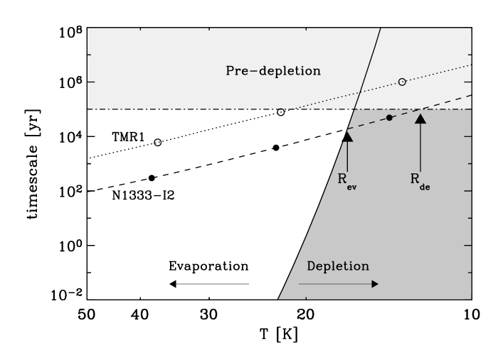
Figure 1: Comparison between CO desorption and freeze-out timescales as functions of temperature and density. The solid line indicates the desorption timescale while the dotted and dashed lines indicate the (density and temperature dependent) freeze-out timescales for TMR1 and N1333-I2, respectively. Depletion occurs where the curves for the freeze-out timescale intersect the dark colored region, in this example for an assumed age of 10⁵ years (dash-dotted line). Freeze-out timescales corresponding to H₂ densities of 1$\times 10^{5}$, 1$\times 10^{6}$ and 1$\times 10^{7}$ cm^-3 for NGC 1333-IRAS2 and 1$\times 10^{4}$, 1$\times 10^{5}$ and 1$\times 10^{6}$ cm^-3 for TMR1 have been indicated by the filled and open circles, respectively.

In order to quantify this scenario, a “drop” abundance structure is introduced as a trial profile, with a depleted abundance $X_{\rm D}$ where $T\leq T_{\rm ev}$ and $n\geq n_{\rm de}$, and an undepleted abundance $X_{0}$ where $T\geq T_{\rm ev}$ or $n\leq n_{\rm de}$. Whereas $T_{\rm ev}$ is in principle a well-defined quantity depending primarily on the ice mantle properties, $n_{\rm de}$ depends on the lifetime of the core compared to the depletion timescale (induced in the pre- and protostellar stages) and the dynamical evolution of the core at earlier stages, including replenishment of undepleted material through infall from larger radii. This may move undepleted envelope material to smaller radii, or higher densities, increasing the derived value of $n_{\rm de}$. On the other hand, within the standard inside-out collapse model (Shu, 1977) the infall radii for these very early stages are so small that the bulk of the envelope is not yet infalling, including the material near the depletion radius where $n=n_{\rm de}$.

For this discussion we only assume step functions at $T_{\rm ev}$ and $n_{\rm de}$, which are thus free parameters together with $X_{0}$ and $X_{\rm D}$. With these assumptions the full Monte Carlo line radiative transfer is performed as described in Jørgensen et al. (2002) and Schöier et al. (2002) using the code of Hogerheijde & van der Tak (2000). We adopt the molecular data summarized in the Leiden Atomic and Molecular Database (Schöier et al., 2005). Single-dish data on CO and HCO⁺ taken from Jørgensen et al. (2002, 2004b) are fitted initially for four objects at different stages of evolution, leaving all 4 parameters free in the modeling of the CO data. The abundance of HCO⁺ is expected to reflect the freeze-out of CO as illustrated by chemical models (e.g., Bergin & Langer, 1997; Lee et al., 2004), but the HCO⁺ lines have higher critical densities and therefore provide an independent probe. Lee et al. modeled the chemical and physical evolution of a collapsing core through its pre- and protostellar stages and found similar “drop profiles” for the CO abundances and closely related species. For the HCO⁺ fits, $T_{\rm ev}$ and $n_{\rm de}$ are therefore taken from the fits to the CO data, giving low values of the $\chi^{2}$-estimator. With $n_{\rm de}$ constrained from fits to the observed CO lines, Eq. (2) then gives the depletion timescale $t_{\rm de}=1/\lambda$ for a source with a given temperature and density profile. Subsequently, the CO data for the entire sample of 16 sources have been fitted, keeping only $X_{\rm D}$ and $n_{\rm de}$ as free parameters.

The pre-stellar cores require a special discussion because they do not have a central source of heating so that there is only a single freeze-out radius $R_{\rm de}$ corresponding to density $n_{\rm de}$. The precise value of $n_{\rm de}$ depends in this case on the adopted physical structure and abundance profile. As an example of the uncertainties, our best-fit models for L1544 are compared with other recent work by Bacmann et al. (2002), Tafalla et al. (2002) and Lee et al. (2003) in Fig. 2, which shows the best fit physical structures together with the derived CO abundance structures. There are some differences in the adopted underlying density profiles and derived parameters. For example, Tafalla et al. (2002) use an exponentially decreasing CO abundance structure toward the center $X(r)=X_{0}\exp(-n(r)/n_{0})$ with $n_{0}=5.5\times 10^{4}$ cm^-3. The origin of the difference between their $n_{0}$ and the lower $n_{\rm de}$ of $1.5\times 10^{4}$ cm^-3 derived using step functions of the CO abundance (Lee et al., 2003, this paper) stems from (i) the slightly lower density profile derived by Evans et al. (2001) and used by Lee et al. and in this paper; (ii) the higher (undepleted) CO abundance in the outer region of the core from Lee et al. and this paper, and (iii) the fact that CO disappears completely in the models of Tafalla et al. at radii less than $\sim 5000$ AU. Lee et al. test different abundance profile types and find that a step function with a characteristic density marked with the vertical arrow in Fig. 2 provides the best fit. Bacmann et al. (2002) derive only an average abundance toward the center of the core with a density profile with a less dense inner flattened region, and therefore do not give constraints on $n_{\rm de}$. Taking this difference in the underlying density profiles into account their average (or constant) CO abundance of 7$\times 10^{-6}$ is in good agreement with the constant abundance of 5$\times 10^{-6}$ for L1544 derived by Jørgensen et al. (2002).

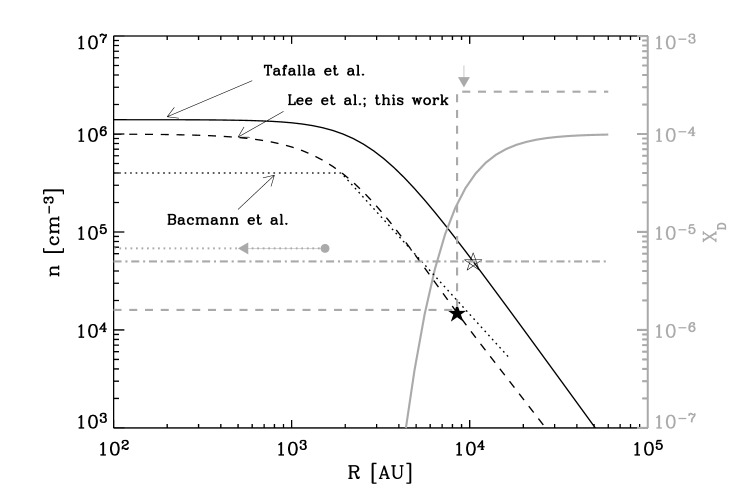
Figure 2: Comparison between the density (black) and CO abundance profiles (grey) from Bacmann et al. (2002) (dotted lines), Tafalla et al. (2002) (solid lines), Lee et al. (2003) and this paper (dashed lines) for the pre-stellar core L1544. The dashed-dotted line indicates the constant abundance from Jørgensen et al. (2002). The freeze-out radius at which a significant drop in the CO abundance occurs in the step-function model of Lee et al. (2003) is indicated by the vertical arrow. The open and solid stars indicate the values of $n_{0}$ (Tafalla et al., 2002) and $n_{\rm de}$ (this work), respectively. See text for details.

3 Results

The best fit parameters to the CO and HCO⁺ data for the 4 sources are listed in Table 1 and illustrated in Fig. 4–5. For the class I object, TMR1, the data are found to be consistent with a model without a depletion zone. For CO, $X_{0}$ is found to be 2.7$\times 10^{-4}$ consistent with the direct measurement of the CO abundance relative to H₂ by Lacy et al. (1994) in a warm cloud in which CO is not frozen out. This is also the expected value based on the results of Jørgensen et al. (2002) who found a maximum constant CO abundance of $\sim$2$\times 10^{-4}$. Van der Tak et al. (2000) found a similar maximum constant abundance for a sample of high-mass YSOs. In the context of the drop abundance model presented in this paper, this constant abundance applies to sources such as TMR1, where the drop region is so small that the abundance profile can be assumed to be essentially constant.

Table 1: Best fit parameters for CO and HCO⁺ lines for the protostars N1333-I2, L723, TMR1 and the pre-stellar core L1544.

	N1333-I2	L723	TMR1	L1544
$T_{\rm ev}$ [K]	$\gtrsim\leavevmode\nobreak\ 35$	40	$\ldots$	$\ldots$
$n_{\rm de}$ [$10^{4}$ cm-3]	7	4	$\ldots$	1.5
CO:
$X_{0}$ [$10^{-4}$]	2.7	2.7	2.7	2.7
$X_{\rm D}$ [$10^{-4}$]	$<$0.14	0.14	$\ldots$	0.02
$\chi^{2}$ / $N$	4.4 / 7	2.4 / 6	0.75 / 6	4.2 / 4
HCO+:
$X_{0}$ [$10^{-8}$]	1.8	$<$2.0	2.7b	–
$X_{\rm D}$ [$10^{-8}$]	0.26	0.35	$\ldots$	–
$\chi^{2}$ / $N$	4.1 / 5	1.8 / 3	2.1b / 2	–
$t_{\rm de}$ [$10^{5}$ yrs]a	2	3	$\lesssim$ 1c	8

Notes: The abundances have been derived from observations of the optically thin isotopic species, C¹⁸O, C¹⁷O and H¹³CO⁺ assuming the standard isotopic ratios adopted in Jørgensen et al. (2004b). ^aDepletion timescale corresponding to the derived $n_{\rm de}$ using Eq. (2). ^bModel including excitation through collisions with electrons at densities $\leq 3\times 10^{4}$ cm^-3. ^c1$\sigma$ limit assuming $T_{\rm ev}$ of 35 K.

For the class 0 objects, in contrast, the constant abundances found by Jørgensen et al. (2002) are about an order of magnitude lower, indicating that the region of CO depletion (the drop zone) is large for these objects. These are also the objects where the intensities of the low excitation $J=1-0$ transitions are underestimated unless the drop abundance structure is introduced. This is clearly illustrated in Fig. 3 which shows the best fit to the C¹⁸O lines for NGC 1333-IRAS2 with a constant abundance model from Jørgensen et al. (2002) and the drop model from this paper. A similar plot illustrating the fits for L723 can be found in Fig. 7 of Jørgensen et al. (2004b). Fig. 4 illustrates the confidence levels for the various parameters for NGC 1333-IRAS2. It is seen that $T_{\rm ev}$ only has a lower limit and $X_{\rm D}$ only an upper limit: for $T_{\rm ev}$ higher than 35–40 K the innermost region with high CO abundances has a very low filling factor in the single-dish beam and therefore only contributes a small fraction to the beam-averaged column densities. The best fit value of $X_{\rm 0}$ is again 2.5–3$\times 10^{-4}$.

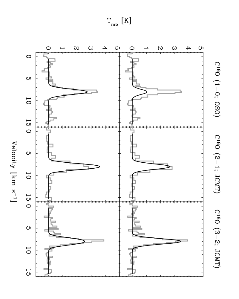
Figure 3: Fitted C¹⁸O line-profiles for NGC 1333-IRAS2. Upper panels: constant fractional abundance [¹²CO] of 2.4$\times 10^{-5}$ from Jørgensen et al. (2002). Lower panel: best fit drop abundance model with $X_{0}=2.7\times 10^{-4}$ and $X_{\rm D}=1.4\times 10^{-5}$ from this paper. The calibrational uncertainty for each observed spectrum is about 20%.

For all sources listed in Table 1 except TMR1, $X_{\rm D}$ is found to be typically an order of magnitude lower than $X_{0}$ for both CO and HCO⁺. The CO evaporation temperatures $T_{\rm ev}$ are all found to be $\geq 35$ K, consistent with the results of Jørgensen et al. (2002), whereas the values of $X_{\rm 0}$ are all of order 2–3$\times 10^{-4}$ with a 10–20% statistical uncertainty.

The derived CO abundance profile depends somewhat on the adopted outer radius and any contribution from the surrounding cloud to the lowest excitation lines. However, the same drop abundance profiles are also necessary to reproduce higher angular resolution interferometer data, where contributions from the larger scale cloud are resolved out, as well as to model transitions with higher critical densities of H₂CO and HCO⁺ which are not excited in the surrounding cloud (Schöier et al., 2004; Jørgensen, 2004, and Table 1).

Given the success of these models, the C¹⁸O and C¹⁷O lines for the entire sample of Jørgensen et al. (2002) have been fitted to infer the CO abundance structure and the depletion time scales. Based on the results for the above 4 sources, it seems reasonable to take the undepleted abundance $X_{0}$ fixed at $2.7\times 10^{-4}$ and the evaporation temperature $T_{\rm ev}$ at 35 K to reduce the number of free parameters. We stress that uncertainties in the underlying physical model such as due to the uncertain dust properties (see discussion in Jørgensen et al., 2002) and other factors may result in systematic uncertainties by factors of 2–3 in the derived absolute abundances and values of $n_{\rm de}$ and $t_{\rm de}$ (see also above example on L1544). However, the conclusion that a drop abundance profile provides a much better fit than a constant abundance profile is not affected by these uncertainties. Also, since all sources are analyzed in the same way, the relative values and inferred trends should be more reliable.

The fitted $n_{\rm de}$ and $X_{\rm D}$, together with the $\chi^{2}$ value and derived $t_{\rm de}$ are given in Table 2. For each source, all lines could be well fitted ($\chi^{2}_{\rm red}\leq 2$) using depletion densities $n_{\rm de}=$1$\times 10^{4}$–6$\times 10^{5}$ cm^-3 ($10^{5\pm 0.4}$ cm^-3) corresponding to depletion timescales of $2\times 10^{4}$–$8\times 10^{5}$ years ($10^{5\pm 0.5}$ years). No significant difference in timescales between Class 0 and I objects is found. For the objects with the least massive envelopes ($M\lesssim 0.1\leavevmode\nobreak\ M_{\odot}$) where photodesorption could become an issue, the derived $t_{\rm de}$ is a lower limit to the actual depletion timescale. In general, however, the depletion radius is located further in the envelope than the radius where $A_{\rm V}=2$ for our objects.

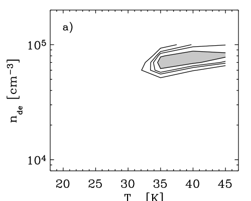
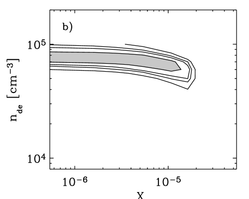
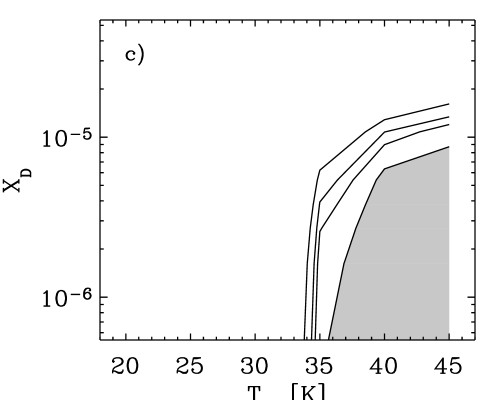
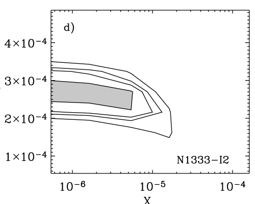
Figure 4: $\chi^{2}$ confidence plots for fits to the CO lines toward NGC 1333-IRAS2. In each plot the grey area marks the 1$\sigma$ confidence region and the subsequent line contours the 2$\sigma$, 3$\sigma$ and 4$\sigma$ confidence regions.

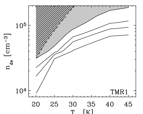
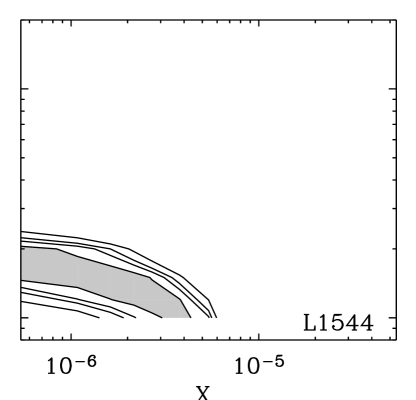
Figure 5: As Fig. 4 but for TMR1 (left) and L1544 (right). In the left panel the dashed region indicates constant abundance models (i.e., models where the radius corresponding to $n_{\rm de}$ is located closer to the central source than the radius corresponding to $T_{\rm ev}$).

Table 2: Values of $n_{\rm d}$ and $X_{\rm D}$ constrained from the CO lines for each individual source in the sample, together with the total $\chi^{2}$, number of fitted lines and derived $t_{\rm de}$.

Source	$n_{\rm de}$	$X_{\rm D}$	$\chi^{2}$ / $N$	$t_{\rm de}$
	[cm-3]			[yr]
L1448-I2	4.8$\times 10^{5}$	3.0$\times 10^{-7}$	4.2 / 4	3$\times 10^{4}$
L1448-C	6.0$\times 10^{4}$	2.0$\times 10^{-5}$	10.7 / 7	2$\times 10^{5}$
N1333-I2	7.0$\times 10^{4}$	1.4$\times 10^{-5}$	4.4 / 7	2$\times 10^{5}$
N1333-I4A	6.0$\times 10^{5}$	2.0$\times 10^{-7}$	11.2 / 7	2$\times 10^{4}$
N1333-I4B	1.7$\times 10^{5}$	4.3$\times 10^{-6}$	9.5 / 7	7$\times 10^{4}$
L1527	1.4$\times 10^{5}$	2.7$\times 10^{-5}$	9.2 / 7	1$\times 10^{5}$
VLA1623a	–	–	–	–
L483b	1.5$\times 10^{5}$	5.0$\times 10^{-6}$	1.5 / 3	9$\times 10^{4}$
L723	4.0$\times 10^{4}$	1.4$\times 10^{-5}$	2.4 / 6	3$\times 10^{5}$
L1157	$<$2.3$\times 10^{5}$	–	–	$>$5$\times 10^{4}$
CB244	1.3$\times 10^{5}$	1.6$\times 10^{-5}$	3.8 / 5	1$\times 10^{5}$
L1489	7.0$\times 10^{4}$	1.0$\times 10^{-5}$	8.1 / 6	1$\times 10^{5}$
TMR1	$\gtrsim$1.0$\times 10^{5}$	–	0.75 / 6	$\lesssim$8$\times 10^{4}$
L1544	1.5$\times 10^{4}$	1.6$\times 10^{-6}$	4.2 / 4	8$\times 10^{5}$
L1689B	$\gtrsim$1.0$\times 10^{4}$	$\lesssim$5$\times 10^{-5}$	0.16 / 3	$\lesssim$1$\times 10^{6}$
IRAS16293c	1.0$\times 10^{5}$	–	–	1$\times 10^{5}$

^aFor VLA1623 the 1–0 line observations are significantly underestimated even for a high constant abundance. This likely reflects the dense ridge of material in which this source is located, which also affects the higher excitation lines (see also discussion in Jørgensen et al., 2002). ^bFrom fits to single-dish and interferometric C¹⁸O observations (Jørgensen, 2004). ^cFrom fits to H₂CO interferometer data (Schöier et al., 2004). The CO isotopic lines for IRAS 16293-2422 are consistent with a constant abundance throughout the envelope but do not rule out a drop in abundance.

4 Discussion

The fact that the drop abundance profiles provide better fits than constant abundance profiles for all sources and molecules studied shows that this structure provides a good representation of the dominant chemistry in protostellar envelopes, with other chemical effects being of secondary importance. To illustrate the dependence on envelope mass, Fig. 6 compares the radii corresponding to $T_{\rm ev}$ and $n_{\rm de}$ for varying envelope masses for a (typical) 3 $L_{\odot}$ central source. For an object with a large envelope mass like NGC 1333-IRAS2 (1.7 $M_{\odot}$), the depletion zone is a few thousand AU, a substantial fraction of the entire envelope. For an object with a small envelope mass like TMR1 (0.1 $M_{\odot}$), the freeze-out radius moves inwards and the size of the depleted region becomes vanishingly small. This indicates that the trend of increasing (constant) abundances with decreasing envelope mass for these species (Jørgensen et al., 2002, 2004b) reflects the size of the depletion region.

Figure 6: Characteristic radii as functions of envelope mass for a 3 $L_{\odot}$ protostar using the models of Jørgensen et al. (2002). An $n\propto r^{-1.5}$ envelope density profile was assumed with inner and outer radii of 25 and 15000 AU, respectively. The dashed line indicate the radius where $T_{\rm ev}=35$ K and the solid and dotted lines the radii where the depletion timescales are 10⁴ and 10⁵ years, respectively. The dashed-dotted line indicates the difference between the depletion and evaporation radii (i.e., size of the depletion zone) for a depletion timescale of 10⁵ years.

Based on the above fits, we propose a chemical structure of the outer envelopes as shown schematically in Fig. 7. The main difference between the pre- and protostellar cores is the inner source of heating in the protostars that causes CO to be evaporated rather than depleted toward the source center. The main difference between the Class 0 and I objects is the size of the depletion zone.

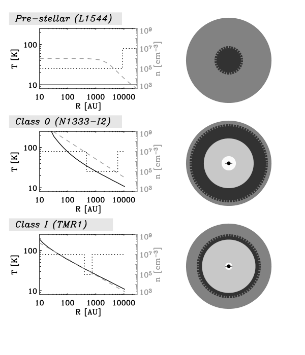
Figure 7: Proposed chemical structure for low-mass pre- and protostellar objects. The left column gives the temperature and density as functions of radius (black solid and grey dashed lines, respectively) for three archetypical low-mass pre- and protostellar objects: L1544 (pre-stellar core), N1333-I2 (class 0, $M_{\rm env}>0.5$ M_⊙ protostar) and TMR1 (class I, $M_{\rm env}<0.5$ M_⊙ protostar). The black dotted lines indicate the derived abundance structures. The right column gives the depletion signature for each class of object with, going from the outside to the inside, the dark grey indicating the region where the density is too low for depletion ($n<n_{\rm de}$), the black indicating the region where the molecules deplete and the light grey indicating the region where they evaporate ($T>T_{\rm ev}$).

Is this chemical structure also an evolutionary indicator? Due to progressive dispersion of the envelope by outflows and mass accretion, an intially massive envelope like that of NGC 1333-IRAS2 should eventually go through a phase with a low-mass envelope like that around TMR1. However, in contrast with the size of the depletion zone, no clear correlation is seen between the derived age $t_{\rm de}$ and derived envelope mass or luminosity for the entire sample (e.g., Table 1). This indicates that the depletion timescales must also reflect other properties, such as the mass of the core from which the protostar is formed. In other words, an other object like TMR1 did not necessarily start out with an envelope as massive as that of NGC 1333-IRAS2. The relatively short timescales of $10^{5\pm 0.5}$ years suggest that the depletion structure is established in the pre-stellar stages, but only after the pre-stellar core has become dense enough that freeze-out really sets in. The rather small scatter seen indicates that this stage is short, of order $10^{5}$ years.

This timescale provides an interesting independent age constraint for the studies of core collapse, since it is shorter than the ages derived from the above mentioned statistical studies (e.g., Lee & Myers, 1999; Jessop & Ward-Thompson, 2000). This apparent discrepancy may reflect simply the definition of the pre-stellar stage: our estimate refers only to the dense pre-stellar phase where depletion has become significant. On the other hand, the statistical studies may be missing low-luminosity embedded infrared sources due to the limited sensitivty of IRAS (see, e.g., Young et al., 2004) and thus lead to overestimates of the timescales. Further unbiased surveys, e.g., with the Spitzer Space Telescope, may shed further light into this issue.

To refine the proposed models, it will be necessary to couple models for the dynamical and radial chemical evolution as done by Lee et al. (2004) to fully address the use of $n_{\rm de}$ as a tracer of age. It is interesting to note that our derived empirical drop abundance structure agrees well with these detailed models, not only qualitatively but also quantitatively. As their Fig. 6 shows, the timescales over which the heavy depletion occurs in the pre- and protostellar stages is only of order $10^{5}$ years.

Another important consequence of the “drop” chemical structure is that it affects the tracers of infall in protostostellar envelopes. Since the dynamical structure of protostellar cores is often inferred from fits of line profiles of molecules such as HCO⁺ (e.g., Gregersen et al., 1997), knowledge about the radial chemical structure is important for detailed descriptions of the infalling envelope. For example, the location of the collapse radius in the inside-out collapse model for the envelope around NGC 1333-IRAS2 (Jørgensen et al., 2004a) is at $\approx 1000$ AU which is in the middle of the drop zone where the temperature is $\approx 25$ K. The exact “infall” line profile will therefore depend critically not only on the velocity field but also the presence and location of the outer pre-depletion ($n<n_{\rm de}$) zone and the amount of depletion.