ADIABATIC AND ENTROPY PERTURBATIONS IN INFLATIONARY MODELS BASED ON NON-LINEAR SIGMA MODEL

N.A. Koshelev¹
Ulyanovsk State University, 42 Leo Tolstoy St., Ulyanovsk 432700, Russia

The scalar perturbations in inflationary models, based on a two-component diagonal non-linear sigma model, are considered. For inhomogeneities generated at an inflationary stage, the law of motion of the comoving curvature ${\cal R}$ is obtained (without using the slow roll approximations). A formal expressions for the power spectrum and its spectral index are obtained, which are valid and after the slow-roll stage. As an example, an inflationary model with a massive scalar field and quadratic curvature corrections is studied numerically.

1 Introduction.

A standard hypothesis of modern cosmology is the existence of an accelerated expansion stage in the history of the very early Universe, when the second time derivative of the scale factor is positive. This expansion was termed inflationary. Presence of a long enough inflationary stage can resolve such well-known difficulties of the Big Bang theory, as the homogeneity, horizon and flatness problems [1]. Besides, the inflationary theory gives a root source of primordial inhomogeneities, giving rise to the large-scale structure of the Universe. In the simple models of chaotic inflation the existence only one scalar field termed inflaton is supposed. In a wide range of initial values of this field, the slow roll conditions is realized, and the scale factor grows quasi exponential. The primordial density inhomogeneities arise from quantum vacuum fluctuations of the inflaton field. These quantum fluctuations, after horizon crossing, can be considered as classical stochastic perturbations [2]. At large scales, the conservation law of the comoving curvature perturbation $\cal{R}$ allows to connect inhomogeneities generated on inflationary stage with primordial inhomogeneities in a radiation-dominated Universe. The slow-roll models predict initial inhomogeneities with an approximately scale-invariant (Harrison - Zel’dovich) spectrum in good agreement with the astrophysical data [3]. However, more realistic multi-field inflationary models also call the attention. In such models, even for long-wavelength inhomogeneities, the conservation law of the quantity $\cal{R}$ may not to hold (for example, strong amplification of long-wavelength inhomogeneities is possible at the preheating stage). Many authors considered the evolution $\cal{R}$ for a number of multi-field models both analytically and numerically. For double-field inflationary models, the equation of motion of the comoving curvature perturbation was written out in the pioneering papers [4], [5].

In this work, we consider inflationary models based on a non-linear sigma model with self-coupling potential. The general two-component diagonal sigma-model action has the form:

$$S=\int d^{4}x\sqrt{|g|}\left\{-\frac{R}{2\kappa^{2}}+\frac{1}{2}T^{2}(\varphi,\chi)\varphi_{;\mu}\varphi^{;\mu}\right.$$

$$+\left.\frac{1}{2}P^{2}(\varphi,\chi)\chi_{;\mu}\chi^{;\mu}-U(\varphi,\chi)\right\},$$ (1)

where the chiral metric components $T^{2}(\varphi,\chi)$, $P^{2}(\varphi,\chi)$ are some functions of chiral fields (sigma model components) $\varphi$ and $\chi$. The non-linear sigma models usually arise after a conformal transformation in generalized Einstein theories [6]. In Refs. [7], [8], inflationary models with an action of such view have received the name of chiral models. They are often call simply multi-field models [9, 10], however, we do not use this term to stress the non-triviality of the scalar fields space.

In two-field inflationary models, to study adiabatic and entropy perturbations, Gordon at al. [11] constructed the quantities $\delta\sigma$ and $\delta s$ . These variables are very convenient for describing the time evolution of the comoving curvature ${\cal R}$, and for solving the perturbed field and Einstein equations in slow roll. The perturbation equations in the new variables are also suitable for numerical simulations [11, 12]. This approach was generalized to the case of a non-linear sigma model with chiral metric components $h_{11}=1$, $h_{12}=0$, $h_{22}={\rm e}^{2b(\varphi_{1})}$ [13], and to the case of the general non-linear sigma model under slow roll conditions [10]. The goal of the presented work is to study the evolution of comoving curvature perturbations and to obtain a power spectrum of initial inhomogeneities in inflationary models with the action (1).

2 Background.

We consider the spatially flat Friedmann - Robertson - Walker (FRW) universe, described by the action (1) with the line element

$$ds^{2}=dt^{2}-a^{2}(t)\delta_{ij}dx^{i}dx^{j}.$$ (2)

The equations of motion for the homogeneous background chiral fields $\varphi$, $\chi$ and scale factor $a(t)$ are

$$H^{2}=\frac{\kappa^{2}}{3}\left({\frac{T^{2}}{2}\dot{\varphi}^{2}+\frac{P^{2}}{2}\dot{\chi}^{2}+U}\right),$$ (3)

$$\dot{H}=-\frac{\kappa^{2}}{2}\left({T^{2}\dot{\varphi}^{2}+P^{2}\dot{\chi}^{2}}\right),$$ (4)

$$\ddot{\varphi}+3H\dot{\varphi}+2\frac{\dot{T}}{T}\dot{\varphi}-\frac{T_{,\varphi}}{T}\dot{\varphi}^{2}-\frac{PP_{,\varphi}}{T^{2}}\dot{\chi}^{2}+\frac{U_{,\varphi}}{T^{2}}=0,$$ (5)

$$\ddot{\chi}+3H\dot{\chi}+2\frac{\dot{P}}{P}\dot{\chi}-\frac{P_{,\chi}}{P}\dot{\chi}^{2}-\frac{TT_{,\chi}}{P^{2}}\dot{\varphi}^{2}+\frac{U_{,\chi}}{P^{2}}=0,$$ (6)

where $H\equiv\frac{\dot{a}}{a}$ is the Hubble rate.

Following the papers [10, 11], we define the new ”adiabatic” field $\sigma$ such that

$$\dot{\sigma}=T\dot{\varphi}\cos\Theta+P\dot{\chi}\sin\Theta,$$ (7)

where

$$\frac{T\dot{\varphi}}{\sqrt{T^{2}\dot{\varphi}^{2}\!+\!P^{2}\dot{\chi}^{2}}}\!=\!\cos\Theta,~{}\frac{P\dot{\chi}}{\sqrt{T^{2}\dot{\varphi}^{2}\!+\!P^{2}\dot{\chi}^{2}}}\!=\!\sin\Theta.$$ (8)

Using definitions

$$U_{\sigma}=\frac{U_{,\varphi}}{T}\cos\Theta+\frac{U_{,\chi}}{P}\sin\Theta,$$

$$U_{s}=\frac{U_{,\chi}}{P}\cos\Theta-\frac{U_{,\varphi}}{T}\sin\Theta,$$ (9)

from the chiral field equations (5) and (6) we can write very useful relations:

$$\ddot{\sigma}+3H\dot{\sigma}+U_{\sigma}=0,$$ (10)

$$\dot{\Theta}=-\frac{U_{s}}{\dot{\sigma}}-\frac{P_{,\varphi}}{T}\dot{\chi}+\frac{T_{,\chi}}{P}\dot{\varphi}.$$ (11)

3 Perturbations.

We investigate scalar linear perturbations about the spatially flat FRW background. The corresponding perturbed line element can in general be written as [14, 15]

$$ds^{2}=(1+2\phi)dt^{2}-2aB_{,i}dx^{i}dt~{}~{}~{}~{}~{}~{}~{}~{}~{}~{}$$

$$-a^{2}\left[(1-2\psi)\delta_{ij}+2E_{,ij}\right]dx^{i}dx^{j}.$$ (12)

The non-linear sigma model components can also be decomposed into a homogeneous background fields $\varphi(t)$, $\chi(t)$ and small inhomogeneities $\delta\varphi$, $\delta\chi$:

$$\varphi({\mathbf{x}},t)=\varphi(t)+\delta\varphi({\mathbf{x}},t),$$

$$\chi({\mathbf{x}},t)=\chi(t)+\delta\chi({\mathbf{x}},t).$$ (13)

Gauge transformations $\tilde{t}=t+\xi^{0}(t,{\mathbf{x}})$, $\tilde{{\mathbf{x}}}={\mathbf{x}}+\xi^{,i}(t,{\mathbf{x}})$, where $\xi^{0}(t,{\mathbf{x}})$, $\xi(t,{\mathbf{x}})$ are the arbitrary scalar functions, allow one to simplify the metric tensor by a suitable choice of constant-time hypersurfaces and spatial coordinates inside them. Here we operate without specified any particular gauge conditions.

Using perturbations of the energy-momentum tensor $\delta T^{\mu}_{\nu}$ and those of the Einstein tensor $\delta G^{\mu}_{\nu}$[14], one can obtain the perturbed Einstein equations for inhomogeneities with the comoving wave number $\mathbf{k}$:

$$3H(H\phi_{\mathbf{k}}+\dot{\psi_{\mathbf{k}}})+\frac{k^{2}}{a^{2}}\left[\psi_{\mathbf{k}}+H(a^{2}\dot{E}_{\mathbf{k}}-aB_{\mathbf{k}})\right]$$

$$=-\frac{\kappa^{2}}{2}\delta\rho_{\mathbf{k}},$$ (14)

$$\dot{\psi}_{\mathbf{k}}+H\phi_{\mathbf{k}}=-\frac{\kappa^{2}}{2}\delta q_{\mathbf{k}},$$ (15)

$$\ddot{\psi}_{\mathbf{k}}+3H\dot{\psi}_{\mathbf{k}}+H\dot{\phi}_{\mathbf{k}}+(2\dot{H}+3H^{2})\phi_{\mathbf{k}}$$

$$=\frac{\kappa^{2}}{2}({\delta\rho_{\mathbf{k}}-2U_{,\varphi}\delta\varphi_{\mathbf{k}}-2U_{,\chi}\delta\chi_{\mathbf{k}}}),$$ (16)

$$\phi_{\mathbf{k}}\!-\psi_{\mathbf{k}}\!+H(aB_{\mathbf{k}}\!-a^{2}\dot{E}_{\mathbf{k}})+(aB_{\mathbf{k}}\!-a^{2}\dot{E}_{\mathbf{k}})^{{\displaystyle{\cdot}}}\!=0,$$ (17)

where the quantities $\delta\rho_{\mathbf{k}}$, $\delta q_{\mathbf{k}}$ are

$$\delta\rho_{\mathbf{k}}=T^{2}\dot{\varphi}\delta\dot{\varphi}_{\mathbf{k}}+(U_{,\varphi}+PP_{,\varphi}\dot{\chi}^{2}+TT_{,\varphi}\dot{\varphi}^{2})\delta\varphi_{\mathbf{k}}$$

$$+P^{2}\dot{\chi}\delta\dot{\chi}_{\mathbf{k}}\!+\!(U_{,\chi}\!+\!PP_{,\chi}\dot{\chi}^{2}\!+\!TT_{,\chi}\dot{\varphi}^{2})\delta\chi_{\mathbf{k}}\!-\!\dot{\sigma}^{2}\phi_{\mathbf{k}},$$ (18)

$$\delta q_{\mathbf{k}}=-T^{2}\dot{\varphi}\delta\varphi_{\mathbf{k}}-P^{2}\dot{\chi}\delta\chi_{\mathbf{k}}.$$ (19)

In studying the evolution of perturbations, gauge-invariant quantities are very convenient. The following gauge-invariant quantities are often used:

$$\Phi=\phi+\left(aB-a^{2}\dot{E}\right)^{\displaystyle{\cdot}},$$

$$\Psi=\psi-H\left(aB-a^{2}\dot{E}\right).$$ (20)

They were constructed by Bardeen [16] and are widely used in the influential report [14]. The comoving curvature perturbation ${\cal R}_{\mathbf{k}}$ can be expressed using the quantities $\Phi_{\mathbf{k}}$ and $\Psi_{\mathbf{k}}$ as follows [17]:

$${\cal R}_{\mathbf{k}}=\Psi_{\mathbf{k}}-\frac{H(H\Phi_{\mathbf{k}}+\dot{\Psi}_{\mathbf{k}})}{\dot{H}}.$$ (21)

Eq. (17) can be rewritten in the simple form

$$\Phi_{\mathbf{k}}=\Psi_{\mathbf{k}}.$$ (22)

Taking a time derivative of Eq. (21), using the background field equations and Eqs. (3) - (17), we find the equation of motion of the comoving curvature perturbation

$$\dot{\cal R}_{\mathbf{k}}=2H\dot{\varphi}\dot{\chi}\frac{T^{2}\dot{\varphi}U_{,\chi}-P^{2}\dot{\chi}U_{,\varphi}}{(T^{2}\dot{\varphi}^{2}+P^{2}\dot{\chi}^{2})^{2}}\left(\frac{\delta\varphi_{\mathbf{k}}}{\dot{\varphi}}-\frac{\delta\chi_{\mathbf{k}}}{\dot{\chi}}\right)$$

$$+\frac{H}{\dot{H}}\frac{k^{2}}{a^{2}}\Psi_{\mathbf{k}}.$$ (23)

In the description of the evolution of the inhomogeneities, we shall also use the new variables $\delta s$ and $\delta\sigma$ [10]:

$$\delta s=P\cos\Theta\delta\chi-T\sin\Theta\delta\varphi,$$

$$\delta\sigma=P\sin\Theta\delta\chi+T\cos\Theta\delta\varphi.$$ (24)

The quantities $\delta\sigma$ and $\delta s$ were termed in Ref. [11] ”adiabatic” and ”entropy” perturbations. As indicated, by the name, perturbations with $\delta s=0$ are only adiabatic. By definition, it is clear that $\delta\sigma$ is associated with inhomogeneities of the field $\sigma$ while $\delta s$ corresponds to inhomogeneities of the entropy field $s$ defined by

$$ds=P\cos\Theta d\chi-T\sin\Theta d\varphi.$$ (25)

In some two-field inflationary models [18], there is a very simple relationship between the generalized entropy perturbations $\delta s$ after inflation and the specific entropy at the start of radiation dominated stage [11, 19].

Using variables $\delta\sigma$ and $\delta s$, Eq. (3) can be reduce to

$$\dot{\cal R}_{\mathbf{k}}=\frac{H}{\dot{H}}\frac{k^{2}}{a^{2}}\Psi_{\mathbf{k}}-2H\frac{U_{s}}{\dot{\sigma}^{2}}\delta s_{\mathbf{k}},$$ (26)

which formally coincides with the corresponding equations of Refs. [11], [13]. For purely adiabatic perturbations ($\delta\varphi/\dot{\varphi}=\delta\chi/\dot{\chi}$), we have $\delta s=0$, and at large scales ($k/a\ll H$), a conservation law is valid for comoving curvature perturbation ${\cal R}_{\mathbf{k}}$.

The perturbed chiral field equations also can be presented in the terms of the new variables. Directly perturbing the chiral field equations [20] for sigma model (1), we find:

$$\ddot{\delta\varphi}_{\mathbf{k}}\!+\!\left(\!3H\!+2\frac{\dot{T}}{T}\!\right)\!\dot{\delta\varphi}_{\mathbf{k}}\!+2\!\left(\!\frac{T_{,\chi}}{T}\dot{\varphi}\!-\frac{PP_{,\varphi}}{T^{2}}\dot{\chi}\!\right)\!\dot{\delta\chi}_{\mathbf{k}}$$

$$+\!\left(\!2\frac{(a^{3}TT_{,\varphi}\dot{\varphi}\dot{)}}{a^{3}T^{2}}\!-\!\frac{(T^{2})_{,\varphi\varphi}}{2T^{2}}\dot{\varphi}^{2}\!-\!\frac{(P^{2})_{,\varphi\varphi}}{2T^{2}}\dot{\chi}^{2}\!\right)\!\delta\varphi_{\mathbf{k}}$$

$$+\!\left(\!2\frac{(a^{3}TT_{,\chi}\dot{\varphi}\dot{)}}{a^{3}T^{2}}\!-\!\frac{(T^{2})_{,\varphi\chi}}{2T^{2}}\dot{\varphi}^{2}\!-\!\frac{(P^{2})_{,\varphi\chi}}{2T^{2}}\dot{\chi}^{2}\!\right)\!\delta\chi_{\mathbf{k}}$$

$$+\left(\frac{k^{2}}{a^{2}}+\frac{U_{,\varphi\varphi}}{T^{2}}\right)\delta\varphi_{\mathbf{k}}+\frac{U_{,\varphi\chi}}{T^{2}}\delta\chi_{\mathbf{k}}+2\frac{U_{,\varphi}}{T^{2}}\phi_{\mathbf{k}}$$

$$=\dot{\varphi}\left(\dot{\phi}_{\mathbf{k}}+3\dot{\psi}_{\mathbf{k}}-\frac{k^{2}B_{\mathbf{k}}}{a}+k^{2}\dot{E}_{\mathbf{k}}\right)\!,$$ (27)

$$\ddot{\delta\chi}_{\mathbf{k}}\!+\!\left(\!3H\!+\!2\frac{\dot{P}}{P}\!\right)\!\dot{\delta\chi}_{\mathbf{k}}\!+2\!\left(\!\frac{P_{,\varphi}}{P}\dot{\chi}\!-\frac{TT_{,\chi}}{P^{2}}\dot{\varphi}\!\right)\!\dot{\delta\varphi}_{\mathbf{k}}$$

$$+\!\left(\!2\frac{(a^{3}PP_{,\chi}\dot{\chi}\dot{)}}{a^{3}P^{2}}\!-\!\frac{(P^{2})_{,\chi\chi}}{2P^{2}}\dot{\chi}^{2}\!-\!\frac{(T^{2})_{,\chi\chi}}{2P^{2}}\dot{\varphi}^{2}\!\right)\!\delta\chi_{\mathbf{k}}$$

$$+\!\left({\!2\frac{(a^{3}PP_{,\varphi}\dot{\chi}\dot{)}}{a^{3}P^{2}}\!-\!\frac{(P^{2})_{,\varphi\chi}}{2P^{2}}\dot{\chi}^{2}\!-\!\frac{(T^{2})_{,\varphi\chi}}{2P^{2}}\dot{\varphi}^{2}}\!\right)\!\delta\varphi_{\mathbf{k}}$$

$$+\left(\frac{k^{2}}{a^{2}}+\frac{U_{,\chi\chi}}{P^{2}}\right)\delta\chi_{\mathbf{k}}+\frac{U_{,\varphi\chi}}{P^{2}}\delta\varphi_{\mathbf{k}}+2\frac{U_{,\chi}}{P^{2}}\phi_{\mathbf{k}}$$

$$=\dot{\chi}\left(\dot{\phi}_{\mathbf{k}}+3\dot{\psi}_{\mathbf{k}}-\frac{k^{2}B_{\mathbf{k}}}{a}+k^{2}\dot{E}_{\mathbf{k}}\right).$$ (28)

After some calculations, the following equations for the inhomogeneities $\delta\sigma_{\mathbf{k}}$ and $\delta s_{\mathbf{k}}$ can be derived:

$$\ddot{\delta\sigma}_{\mathbf{k}}\!+\!3H\dot{\delta\sigma}_{\mathbf{k}}\!+\!\left(\!\frac{k^{2}}{a^{2}}\!+\!\frac{U_{s}}{\dot{\sigma}}\dot{\Theta}\!+\!U_{\sigma\sigma}\!-\!\frac{U_{,\chi}}{\dot{\sigma}}\frac{\dot{P}}{P^{2}}\sin\Theta\right.$$

$$\left.-\frac{U_{,\varphi}}{\dot{\sigma}}\frac{\dot{T}}{T^{2}}\cos\Theta\!\right)\!\delta\sigma_{\mathbf{k}}+2\left(\!\frac{U_{s}}{\dot{\sigma}}\delta s_{\mathbf{k}}\!\right)^{\displaystyle{\cdot}}\!-2\frac{U_{\sigma}}{\dot{\sigma}}\frac{U_{s}}{\dot{\sigma}}\delta s_{\mathbf{k}}$$

$$=-2U_{\sigma}\phi_{\mathbf{k}}+\dot{\sigma}\left(\dot{\phi}_{\mathbf{k}}+3\dot{\psi}_{\mathbf{k}}+k^{2}\dot{E}_{\mathbf{k}}-\frac{k^{2}B_{\mathbf{k}}}{a}\right)\!,$$ (29)

$$\ddot{\delta s}_{\mathbf{k}}+3H\dot{\delta s}_{\mathbf{k}}+\left(\frac{U_{\sigma}}{PT}\left(P_{,\varphi}\cos\Theta+T_{,\chi}\sin\Theta\right)\right.$$

$$+\left(\frac{P_{,\varphi}T_{,\varphi}}{T^{2}}+\frac{P_{,\chi}T_{,\chi}}{P^{2}}-\frac{P_{,\varphi\varphi}}{T}-\frac{T_{,\chi\chi}}{P}\right)\frac{\dot{\sigma}^{2}}{PT}$$

$$+\frac{U_{,\chi}}{P^{2}}\cos\Theta\left(\frac{P_{,\varphi}}{T}\sin\Theta-\frac{P_{,\chi}}{P}\cos\Theta\right)$$

$$-\frac{U_{,\varphi}}{T^{2}}\sin\Theta\left(\frac{T_{,\varphi}}{T}\sin\Theta-\frac{T_{,\chi}}{P}\cos\Theta\right)$$

$$\left.+\frac{k^{2}}{a^{2}}+3\left(\frac{U_{s}}{\dot{\sigma}}\right)^{2}+U_{ss}\right)\delta s_{\mathbf{k}}=2\frac{U_{s}}{\dot{\sigma}^{2}}\epsilon_{m},$$ (30)

where

$$U_{ss}=\frac{U_{,\chi\chi}}{P^{2}}\cos^{2}\Theta-\frac{U_{,\varphi\chi}}{PT}\sin 2\Theta+\frac{U_{,\varphi\varphi}}{T^{2}}\sin^{2}\Theta,$$ (31)

$$U_{\sigma\sigma}=\frac{U_{,\chi\chi}}{P^{2}}\sin^{2}\Theta+\frac{U_{,\varphi\chi}}{PT}\sin 2\Theta+\frac{U_{,\varphi\varphi}}{T^{2}}\cos^{2}\Theta.$$ (32)

Here we use the gauge-invariant quantity $\epsilon_{m}\equiv\delta\rho_{\mathbf{k}}-3H\delta q_{\mathbf{k}}$ [16], the comoving density perturbation:

$$\epsilon_{m}=\dot{\sigma}\left[\dot{\delta\sigma_{\mathbf{k}}}+2\frac{U_{s}}{\dot{\sigma}}\delta s_{\mathbf{k}}-\dot{\sigma}\phi_{\mathbf{k}}-\frac{\ddot{\sigma}}{\dot{\sigma}}\delta\sigma_{\mathbf{k}}\right].$$ (33)

Since from the Eqs. (3) and (15) we have

$$\frac{k^{2}}{a^{2}}\Psi_{\mathbf{k}}=-\frac{\kappa^{2}}{2}\epsilon_{m},$$ (34)

at large scales ($k/a\ll H$) the right hand side of Eq. (3) becomes negligible. As follows from Eq. (3), the large-scale entropy perturbations are decoupled from adiabatic and metric perturbations, which generalizes the conclusion of Ref. [11] on inflationary models with the action (1).

Eq. (3) can be rewritten as an equation for Sasaki-Mukhanov gauge-invariant variable

$$Q=\delta\sigma+\frac{\dot{\sigma}}{H}\psi.$$ (35)

Using this quantity, one can obtain:

$$\ddot{Q}_{\mathbf{k}}+3H\dot{Q}_{\mathbf{k}}+\left(\frac{k^{2}}{a^{2}}+\frac{U_{s}}{\dot{\sigma}}\dot{\Theta}-\frac{U_{,\chi}}{\dot{\sigma}}\frac{\dot{P}}{P^{2}}\sin\Theta\right.$$

$$\left.-\frac{U_{,\varphi}}{\dot{\sigma}}\frac{\dot{T}}{T^{2}}\cos\Theta-\frac{\kappa^{2}}{a^{3}}\left(\frac{a^{3}\dot{\sigma}^{2}}{H}\right)^{\displaystyle{\cdot}}+U_{\sigma\sigma}\!\right)\!Q_{\mathbf{k}}$$

$$=-2\left(\frac{U_{s}}{\dot{\sigma}}\delta s_{\mathbf{k}}\right)^{\displaystyle{\cdot}}+2\left(\frac{U_{\sigma}}{\dot{\sigma}}+\frac{\dot{H}}{H}\right)\frac{U_{s}}{\dot{\sigma}}\delta s_{\mathbf{k}}.$$ (36)

Eqs. (3) and (3) in specific case $T^{2}=1$, $P^{2}=P^{2}(\varphi)$ coincide with the corresponding equations of Ref. [13], and in the slow roll conditions reduce to equations of Ref. [10].

4 Application to slow roll inflationary models.

Let us consider an application of the above expressions to slow roll inflationary models. Quantum vacuum fluctuations of chiral fields become classical inhomogeneities after they leave the horizon. The Fourier component of chiral fields perturbations at horizon crossing are given by [5]

$$\delta\varphi_{\mathbf{k}}(t_{\mathbf{k}})=\frac{1}{T(t_{\mathbf{k}})}\frac{{H(t_{\mathbf{k}})}}{\sqrt{2k^{3}}}e_{\varphi}({\mathbf{k}}),$$ (37)

$$\delta\chi_{\mathbf{k}}(t_{\mathbf{k}})=\frac{1}{P(t_{\mathbf{k}})}\frac{H(t_{\mathbf{k}})}{\sqrt{2k^{3}}}e_{\chi}({\mathbf{k}}).$$ (38)

Here $t_{\mathbf{k}}$ is the instant of horizon crossing ($a(t_{\mathbf{k}})H(t_{\mathbf{k}})$ $=k$), and $e_{\varphi}$, $e_{\chi}$ are real Gaussian stochastic variables with the following properties:

$$\left\langle{e_{\varphi}(\mathbf{k})e_{\chi}(\mathbf{k}^{\prime})}\right\rangle=\delta_{\varphi\chi}\delta^{(3)}\left(\mathbf{k}-\mathbf{k}^{\prime}\right),$$ (39)

$$\left\langle{e_{\phi}(\mathbf{k})}\right\rangle=\left\langle{e_{\chi}(\mathbf{k})}\right\rangle=0.$$ (40)

From (3) and (37) one can derive the following expressions for $\delta\sigma_{\mathbf{k}}$ and $\delta s_{\mathbf{k}}$:

$$\delta\sigma_{\mathbf{k}}(t_{\mathbf{k}})=\frac{{H(t_{\mathbf{k}})}}{\sqrt{2k^{3}}}e_{\sigma}({\mathbf{k}}),~{}\delta s_{\mathbf{k}}(t_{\mathbf{k}})=\frac{H(t_{\mathbf{k}})}{\sqrt{2k^{3}}}e_{s}(\mathbf{k}),$$ (41)

where $e_{\sigma}$, $e_{s}$ are independent Gaussian random quantities with zero average and unit dispersion.

Being restricted to the most important non-decreasing modes of long-wavelength inhomogeneities, as well as in case of single-field inflationary models, it is possible to write the inequality:

$$\dot{\Phi}_{\mathbf{k}}\ll H\Phi_{\mathbf{k}}.$$ (42)

Another standard assumption is that, for non-decreasing modes in the slow-roll regime $|\ddot{\delta\varphi}/\dot{\delta\varphi}|\ll 3H$, $|\ddot{\delta\chi}/\dot{\delta\chi}|\ll 3H$ and therefore [11], [10]

$$|\ddot{\delta\sigma}|\ll 3H|\dot{\delta\sigma}|,~{}~{}~{}~{}~{}~{}~{}~{}~{}~{}|\ddot{\delta s}|\ll 3H|\dot{\delta s}|.$$ (43)

This allows us to disregard $\ddot{\delta\sigma}$ and $\ddot{\delta\sigma}$ in the perturbed field equations (3), (3). Thus, Eq. (3) may be written as

$$\dot{\delta s}_{\mathbf{k}}=A(t)\delta s_{\mathbf{k}},$$ (44)

where

$$A(t)=-\frac{1}{3H}\left(\frac{U_{\sigma}}{PT}\left(P_{,\varphi}\cos\Theta+T_{,\chi}\sin\Theta\right)\right.$$

$$+3\left(\frac{U_{s}}{\dot{\sigma}}\right)^{2}+\frac{U_{,\chi}}{P^{2}}\cos\Theta\left(\frac{P_{,\varphi}}{T}\sin\Theta-\frac{P_{,\chi}}{P}\cos\Theta\right)$$

$$+U_{ss}-\frac{U_{,\varphi}}{T^{2}}\sin\Theta\left(\frac{T_{,\varphi}}{T}\sin\Theta-\frac{T_{,\chi}}{P}\cos\Theta\right)$$

$$\left.+\left(\frac{P_{,\varphi}T_{,\varphi}}{T^{2}}+\frac{P_{,\chi}T_{,\chi}}{P^{2}}-\frac{P_{,\varphi\varphi}}{T}-\frac{T_{,\chi\chi}}{P}\right)\frac{\dot{\sigma}^{2}}{PT}\right).$$ (45)

Taking into account the inequality (42), equations (15) and (21) can be simplified:

$$\Phi_{\mathbf{k}}(t)=\frac{\kappa^{2}}{2H}\dot{\sigma}\delta\sigma_{\mathbf{k}},$$ (46)

$${\cal R}_{\mathbf{k}}=-\frac{H^{2}}{\dot{H}}\Phi_{\mathbf{k}}.$$ (47)

Integrating Eq. (26), one can obtain the following expression for the long-wavelength comoving curvature perturbation ${\cal R}_{\mathbf{k}}$ :

$${\cal R}_{\mathbf{k}}(t)={\cal R}_{\mathbf{k}}(t_{\mathbf{k}})-\frac{H(t_{\mathbf{k}})}{\sqrt{2k^{3}}}J(t,t_{\mathbf{k}})e_{s}({\mathbf{k}}),$$ (48)

where

$$J(t,t_{\mathbf{k}})=\!\!\int_{t_{\mathbf{k}}}^{t}\!\frac{2HU_{s}}{\dot{\sigma}^{2}}\frac{\delta s}{\delta s(t_{\mathbf{k}})}dt=\!\!\int_{t_{\mathbf{k}}}^{t}\!\frac{2HU_{s}}{\dot{\sigma}^{2}}\alpha_{\mathbf{k}}(t)dt.$$ (49)

Here the function $\alpha_{\mathbf{k}}(t)$ is a solution of Eq. (44), normalized by the condition $\alpha_{\mathbf{k}}(t_{\mathbf{k}})=1$. Using first of relations (41), background equation (4) and also equations (46), (47) one can therefore write:

$${\cal R}_{\mathbf{k}}(t)=\frac{H(t_{\mathbf{k}})}{\sqrt{2k^{3}}}\!\left(\!\frac{H(t_{\mathbf{k}})}{\dot{\sigma}(t_{\mathbf{k}})}e_{\sigma}({\mathbf{k}})-J(t,t_{\mathbf{k}})e_{s}({\mathbf{k}})\!\right)\!.$$ (50)

The power spectrum [15] can now be written in the following form:

$${\cal P}_{\cal R}(t)=\frac{H^{2}(t_{\mathbf{k}})}{4\pi^{2}}\left(\frac{H^{2}(t_{\mathbf{k}})}{\dot{\sigma}^{2}(t_{\mathbf{k}})}+J^{2}(t,t_{\mathbf{k}})\right).$$ (51)

This formula is valid also after the slow-roll stage if, for finding the function $\alpha_{\mathbf{k}}(t)$ a long-wavelength limit of Eq. (3) is used instead of Eq. (44). If, from certain time, the entropy perturbation $\delta s$ is so small, that the comoving curvature perturbation ${\cal R}$ remains actually constant, the expression obtained above describe the adiabatic power spectrum.

A commonly used characteristic of a power spectrum is its spectral index $n_{s}$ [15]. Using (51) and background equations one can conclude, that the spectral index for inflationary models under consideration is given by:

$$n_{s}-1\equiv\frac{\partial\ln{\cal P}_{\cal R}(t)}{\partial\ln k}=\frac{1}{H}\frac{\partial\ln{\cal P}_{\cal R}(t)}{\partial t_{\mathbf{k}}}=2\frac{\dot{H}(t_{\mathbf{k}})}{H^{2}(t_{\mathbf{k}})}$$

$$-\frac{\kappa^{2}+\frac{2H(t_{\mathbf{k}})\ddot{\sigma}(t_{\mathbf{k}})}{\dot{\sigma}^{3}(t_{\mathbf{k}})}+2\left(\frac{2U_{s}(t_{\mathbf{k}})}{\dot{\sigma}^{2}(t_{\mathbf{k}})}J+\frac{A(t_{\mathbf{k}})}{H(t_{\mathbf{k}})}J^{2}\right)}{\frac{H^{2}(t_{\mathbf{k}})}{\dot{\sigma}^{2}(t_{\mathbf{k}})}+J^{2}}.$$ (52)

The spectral index is time-dependent due the time-dependence of the quantity $J(t,t_{\mathbf{k}})$.

Eqs. (51), (26), (3) and (3) are the main results of this work. These equations are very well suitable for numerical calculations of perturbation evolution in inflationary models based on non-linear sigma models.

4.1 Numerical example.

As an example, we shall describe an inflationary model with a single massive scalar field and additional higher order curvature terms due to curvature squared. The corresponding action looks like:

$$S=\int d^{4}x\sqrt{|\tilde{g}|}\left\{-\frac{\tilde{R}}{2\kappa^{2}}+\frac{\tilde{R}^{2}}{2\kappa^{2}M^{2}}\right.$$

$$\left.+\frac{1}{2}\varphi_{;\mu}\varphi_{;\nu}\tilde{g}^{\mu\nu}-\frac{1}{2}m^{2}\varphi^{2}\right\}.$$ (53)

Figure 1: The time dependence of ${\cal P}(t)/{\cal P}(t_{\mathbf{k}})$ with $M/m=5$, $\varphi(t_{\mathbf{k}})=14/\kappa$, $\chi(t_{\mathbf{k}})=4/\kappa$.

Making the conformal transformation $g_{ij}=\Omega^{2}\tilde{g}_{ij}$ with $\Omega^{2}=1-\frac{\tilde{R}^{2}}{3M^{2}}$, one gets the action in the Einstein frame:

$$S=\!\!\int\!d^{4}x\sqrt{|g|}\!\left\{\!\frac{-R}{2\kappa^{2}}\!+\!\frac{1}{2}\chi_{;\mu}\chi^{;\mu}\!\!+\!\frac{e^{-\sqrt{\frac{2}{3}}\kappa\chi}}{2}\varphi_{;\mu}\varphi^{;\mu}\right.$$

$$\left.-\frac{3}{4}\frac{M^{2}}{\kappa^{2}}\left[1\!-\!e^{-\sqrt{\frac{2}{3}}\kappa\chi}\right]^{2}\!-\!\frac{1}{2}e^{-2\sqrt{\frac{2}{3}}\kappa\chi}m^{2}\varphi^{2}\!\right\}\!,$$ (54)

where the new field $\chi\equiv\sqrt{3/2}{\kappa}^{-1}\ln\left(1-{\tilde{R}^{2}}/{3M^{2}}\right)$ is introduced. Note that when $\chi\ll\kappa^{-1}$, then $U(\varphi,\chi)\approx M^{2}\chi^{2}/2+m^{2}\varphi^{2}/2$. Some inflationary models more general than (4.1) were considered earlier in the preheating context in [21, 22] (These papers took into account not only higher curvature terms, but also a possible non-minimal coupling $\xi\varphi^{2}\tilde{R}$).

We are interesting here in the case when the chiral fields $\varphi$ and $\chi$ are comparable in magnitude and are both in a slow-roll regime at the beginning of the inflationary stage. In the analysis of the background and inhomogeneities evolution, we shall be restricted to the parameter area $M>m$. Since the field $\chi$ is heavier, it breaks up faster than field $\varphi$, and soon after the inflation influence of the field $\chi$ on the scale factor dynamic and evolution of inhomogeneities is vanishingly small. Besides, after inflation, $\Omega^{2}\cong 1$, therefore actions in the original frame (4.1) and in the Einstein frame (4.1) almost do not differ. Accordingly, the inhomogeneities calculated in both frames after inflation asymptotically coincide. It is clear that the inhomogeneities in this model after the inflationary stage are to a great extent adiabatic.

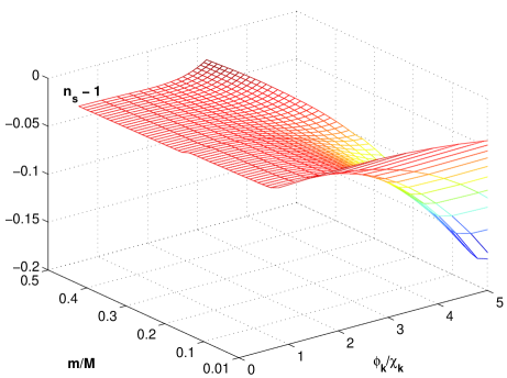
Figure 2: Numerical simulations of the spectral index after inflation. Here it is assumed that the perturbations leave the horizon 60 e-folds before the end of inflation; the inflation ends when $\dot{H}/3H^{2}=1$.

The background and perturbed equations for the sigma model (4.1) can be solved by numerical simulations. For finding the long-wavelength comoving curvature perturbation ${\cal R}$ generated on inflationary stage, it is very convenient to use Eqs. (26) and (3). Eq. (3) is much easier to solve than the initial set of perturbed Einstein and field equations. It can be made by using standard packages of numerical computations. The results of the calculations are presented in Figs. 1 and 2. These pictures show the time dependence ${\cal P}(t)/{\cal P}(t_{\mathbf{k}})$ for a specific choice of parameters and the dependence of the spectral index on the model parameters.

4.2 Acknowledgement.

I thank S.V. Chervon and V.M. Zhuravlev for attention to the work and useful discussions.

References

• [1] A.D. Linde, ” Particle Physics and Inflationary Cosmology”, Harwood, Chur, Switzerland,1990.
• [2] D. Polarski and A.A. Starobinsky, Class. Quant. Grav. 13 377 (1996); gr-qc/9504030.
• [3] S.L. Bridle, A.M. Lewis, J. Weller, G. Efstathiou, MNRAS 342 L72 (2003); astro-ph/0302306.
• [4] J. García-Bellido and D. Wands, Phys. Rev. D 52 6739 (1995); gr-qc/9506050.
• [5] J. García-Bellido and D. Wands, Phys. Rev. D 53 5437 (1996); astro-ph/9511029.
• [6] K. Maeda, Phys. Rev. D 39, 3159 (1989).
• [7] S.V. Chervon, IJMP A 17, 4451-4456 (2002).
• [8] S.V. Chervon, N.A. Koshelev Grav.& Cosmol. 9 196-202 (2003).
• [9] M. Sasaki and E. D. Stewart, Prog. Theor. Phys. 95 71 (1996) ; astro-ph/9507001.
• [10] S. Groot Nibbelink, B. J. W. van Tent, Class. Quant. Grav. 19 613-640 (2002); hep-ph/0107272.
• [11] C. Gordon, D. Wands, B.A. Bassett and R. Maartens, Phys. Rev. D 63 023506 (2001); astro-ph/0009131.
• [12] S. Tsujikawa, B.A. Bassett, Phys.Lett. B 536 9-17 (2002); astro-ph/0204031.
• [13] F. Di Marco, F. Finelli, R. Brandenberger, Phys. Rev. D 67 063512 (2003); astro-ph/0211276.
• [14] V.F. Mukhanov, H.A. Feldman and R.H. Brandenberger, Phys. Rep. 215, 393 (1992).
• [15] A.R. Liddle and D. Lyth, Phys. Rep. 231 p 1 (1993); astro-ph/9303019.
• [16] J.M. Bardeen, Phys. Rev. D 22, 1882 (1980).
• [17] D.H. Lyth, Phys. Rev. D 31 1792 (1985).
• [18] D. Polarski, A.A. Starobinsky, Phys. Rev. D 50, 6123 (1994); astro-ph/9404061.
• [19] D. Langlois, Phys. Rev. D 59, 123512 (1999); astro-ph/9906080.
• [20] S.V. Chervon, Grav.& Cosmol. 8 Suppl. I 32-40 (2002).
• [21] S. Tsujikawa, K.Maeda and T. Torii,Phys. Rev. D 60, 123505 (1999); hep-ph/9906501.
• [22] A.A. Starobinsky, S. Tsujikawa and J. Yokoyama, Nucl. Phys. B 610 383 (2001); astro-ph/0107555.