Observations of the Blandford-Znajek and the MHD Penrose processes in computer simulations of black hole magnetospheres
Abstract
In this paper we report the results of axisymmetric relativistic MHD simulations for the problem of Kerr black hole immersed into a rarefied plasma with ”uniform” magnetic field. The long term solution shows properties which are significantly different from those of the initial transient phase studied recently by Koide(2003). The topology of magnetic field lines within the ergosphere is similar to that of the split-monopole model with a strong current sheet in the equatorial plane. Closer inspection reveals a system of isolated magnetic islands inside the sheet and ongoing magnetic reconnection. No regions of negative hydrodynamic ”energy at infinity” are seen inside the ergosphere and the so-called MHD Penrose process does not operate. Yet, the rotational energy of the black hole continues to be extracted via purely electromagnetic mechanism of Blandford and Znajek(1977). However, this is not followed by development of strong relativistic outflows from the black hole. Combined with results of other recent simulations this signals a potential problem for the standard MHD model of relativistic astrophysical jets should they still be observed at distances as small as few tens of gravitational radii from the central black hole.
keywords:
black hole physics – magnetic fields – methods:numerical.1 Introduction
Observations of various astrophysical phenomena such as active galactic nuclei and galactic microquasars often reveal powerful relativistic jets streaming away from a massive central object, most likely a black hole. The exact mechanism of generating powerful relativistic jets from black holes system is not yet known, although a number of interesting models have been put forward and studied with various degree of detail during the last few decades.
By now there has emerged a general consensus that the central engine should involve a rotating black hole linked with the jets by means of strong magnetic field and an accretion disc supporting this magnetic field by its electric currents. This magnetic field is believed to serve a number of key functions: 1) to power the jets via extracting the rotational energy of the black hole; 2) to provide the jet collimation via magnetic hoop stress; and 3) to suppress mixing of the rarefied jet plasma with the relatively dense surrounding medium such as the coronal plasma of the accretion disc, which is needed to ensure that the jet plasma remains magnetically dominated and, thus, can be accelerated to the ultra-relativistic speeds inferred from the observations.
The most simplified mathematical frameworks for highly magnetised relativistic plasma are an ideal relativistic magnetohydrodynamics (MHD) and magnetodynamics (MD, which can be described as MHD in the limit of zero particle inertia, e.g Komissarov 2002). Both frameworks, however, involve rather complex equations particularly in the case of curved spacetime. This explains a relatively slow progress in the theory – only a limited number of analytical solutions have been found so far and only for the limiting case of a slowly rotating black hole where one can employ the perturbation method. The most important of them is the MD solution for a monopole magnetosphere by Blandford and Znajek (1977). Indeed, this solution describes an outgoing Poynting flux from a Kerr black hole as if the hole was a magnetized rotating conductor whose rotational energy can be efficiently extracted by means of magnetic torque. This most important feature of the Blandford-Znajek solution (BZ) is also the most intriguing and puzzling as such conductor does not really exist.
Often, this missing element of the BZ model is artificially introduced in the form of the so-called “membrane”, or the “stretched horizon”, located somewhat above the real event horizon [Macdonald & Thorne 1982, Thorne et al.1986]. This ”physical” interpretation of the BZ solution provides simple means of communicating the results to wide astrophysical community and for this reason it has been almost universally accepted. However, its artificial nature and the fact that no proper physical interpretation had been pushed forward also made the result vulnerable to criticism on theoretical grounds and stimulated attempts to find alternative ways of magnetic extraction of rotational energy of black holes [Punsly & Coroniti 1990a, Punsly 2001, Takahashi et al.1990]. These attempts seem to draw the inspiration from a completely non-magnetic mechanism proposed much earlier by Penrose (1969). The key role in this mechanism is played by the ergosphere of a rotating black hole. Within the ergosphere particles can acquire negative energy (or rather ”energy at infinity”) and if such particles are swallowed by the black hole its energy can decrease. In the original Penrose process such particles are created via close range interaction (collisions, decay) with other particles which gain positive energy and carry it away. However, electrically charged particles can also be pushed onto orbits with negative energy by the Lorentz force and this is what makes possible the so-called ”MHD Penrose process” [Takahashi et al.1990, Koide et al.2002, Koide 2003] which is the common element of all alternative magnetic mechanisms.
Recently there has been a renewed interest to this problem. The main reason for this is the arrival of robust numerical methods for relativistic astrophysics, e.g. [Pons et al.1998, Komissarov 1999, Koide et al.1999, Koldoba et al.2002, Gammie et al.2003, Del Zanna et al.2003, De Villiers & Hawley 2003]. Time-dependent MD and MHD simulations of monopole magnetospheres of black holes have demonstrated the asymptotic stability of the BZ solution [Komissarov 2001] and provided additional arguments in favour of the MD approximation in this particular case [Komissarov 2004a, Komissarov 2004b]. Moreover, simulations of magnetically driven accretion disks have shown the development of low density axial regions, ”funnels”, closely described by the BZ solution [De Villiers et al. 2003, McKinney & Gammie 2004].
On the other hand, the MHD simulations of a black hole immersed into a rarefied plasma with uniform magnetic field seemed to provide support for the MHD Penrose model [Koide et al.2002, Koide 2003]. At least, it was found that by the end of the simulations the inflow of particles with negative energy at infinity accounted for about one half of the extracted energy. Unfortunately, the termination time of these simulations was surprisingly short, approximately one half of the rotational period of the black hole (presumably due to some computational problems.) As the result one could not tell whether the MHD Penrose mechanism would remain effective on a long-term basis. In this paper we present the results of new simulations which were carried out for much longer period of time and which bring new light on this important issue.
2 Basic equations and numerical method
In these simulations we solve numerically the equations of ideal MHD in the space-time of a Kerr black hole. This space-time is described using the foliation approach where the time coordinate parametrises a suitable filling of spacetime with space-like hypersurfaces described by the 3-dimensional metric tensor . These hypersurfaces may be regarded as the “absolute space” at different instances of time . If are the spatial coordinates of the absolute space then the metric form can be written as
| (1) |
where is called the “lapse function” and is the “shift vector”. In this study we employ the Kerr-Schild coordinates, , which like the well known Boyer-Lindquist coordinates ensure that none of the components of the metric form depend on and . At spatial infinity these coordinate systems do not differ but the Kerr-Schild system does not have a coordinate singularity on the event horizon. Other details can be found in e.g. [Komissarov 2004a, McKinney & Gammie 2004].
The evolution equations of ideal MHD include the continuity equation,
| (2) |
the energy-momentum equations,
| (3) |
and the induction equation,
| (4) |
Here is the metric tensor of spacetime,
,
is the Levi-Civita
pseudo-tensor of space, is the proper mass density of plasma,
is its four-velocity vector. The total stress-energy-momentum
tensor, , is a sum of the stress-energy momentum tensor of
matter,
| (5) |
where is the thermodynamic pressure and is the enthalpy per unit volume, and the stress-energy momentum tensor of electromagnetic field,
| (6) |
where is the Maxwell tensor of the electromagnetic field. The electric field, , and the magnetic field, , are defined via
| (7) |
and
| (8) |
where is the Faraday tensor of the electromagnetic field, which is simply dual to the Maxwell tensor. In the limit of ideal MHD
| (9) |
where is the usual 3-velocity of plasma. In addition, the magnetic field must satisfy the divergence free condition
| (10) |
Note, that 1) all the components of vectors and tensors appearing in these equations are the those measured in the coordinate basis, , of the Kerr-Schild coordinates; 2) throughout the paper we employ such units that the speed of light , the gravitational constant , the black hole mass , and the factor does not appear in Maxwell’s equations.
Our numerical scheme is a 2D Godunov-type upwind scheme which utilises special relativistic Riemann solver described in Komissarov(1999) and uses the method of constraint transport [Evans & Hawley 1988] to preserve the magnetic field divergence free. Other details are outlined in [Komissarov 2004b].
3 Numerical simulations
3.1 Setup
In these simulations the rotational parameter of the Kerr metric is which gives the event horizon radius . The axisymmetric computational domain covers and . The computational grid has 401 cells in the -direction, where it is uniform, , and 400 cells in the -direction. The cell size in the -direction, , is such that the corresponding physical lengths in both directions are equal in the equatorial plane.
The usual axisymmetric boundary conditions are imposed at and boundaries. At the outer boundary, , the initial values of all variables are imposed throughout the whole run, the termination time for the simulations was set to so no waves emitted from the dynamically active region near the black hole had a chance to get reflected of the boundary and effect the inner solution. The inner boundary is well inside the event horizon, which justifies use of “radiative boundary conditions”.
The initial velocity field is set to be the same as the one of the fiducial observers of the Kerr-Schild foliation, who spiral towards the black hole (e.g. Komissarov 2004a).
The initial electromagnetic field has the same “uniform” magnetic component, aligned with the rotational axis of the black hole, as in the vacuum solution of Wald:
| (11) |
where and are the Killing vectors of the Kerr spacetime [Wald 1974]. However, the initial electric component is different as it has to satisfy the condition of perfect conductivity (9).
The initial thermodynamic pressure and the rest mass density of plasma are set to be and , where is the magnetic pressure. Finally, the equation of state employed in the simulations describes polytropic gas with the ratio of specific heats, .
Summarising, although the setup of our simulations is not exactly the same as in Koide[Koide 2003] it is quite similar. In both cases we are dealing with magnetically dominated plasma of similar magnetisation. In both cases the initial magnetic field is described by the Wald vacuum solution [Wald 1974]. Thus one would expect to obtain at least qualitatively similar solution in the common region of computational domains. Because of different space-time foliations, Koide[Koide 2003] used the Boyer-Lindquist coordinates, the difference in computational domains is not simply reduced to the difference in the range of the radial coordinate, . Different definitions of the global time coordinate, , should also be taken into account. This, however, is only significant in the spacial regions very close to the event horizon where the Boyer-Lindquist system becomes singular.
All conservative schemes for the relativistic magnetohydrodynamics have an upper limit on plasma magnetization above which they fail. At this limit, which somewhat varies from problem to problem and also depends on the resolution, the numerical error for the total energy density becomes comparable with the energy density of matter. This forces us to pump in fresh plasma in regions where its magnetization becomes dangerously high. Since in such regions the dynamical role of particles is rather insignificant this measure should not have a strong effect in most respects. The critical condition we set in these simulations is
| (12) |
where is the Lorentz factor of the flow and is the magnetic field strength as measured by the local FIDO. Should the energy density of matter drop below , both and are artificially increased by the same factor. To minimise the effect of the mass injection on the flow the velocity of the injected matter is set to be equal to the local velocity of the flow. In fact, new particles must be constantly created in real magnetospheres of black holes but the details of this process can be rather different [Beskin et al.1991, Hirotani & Okamoto 1998, Phinney 1982]. An additional lower limit was set on the value of the thermodynamic pressure, which was not allowed to drop below .
3.2 Results and Discussion
We have found that numerical solution exhibits two phases with rather different properties: 1) the rather short initial phase which is dominated by a rapid evolution in the neighbourhood of the black hole and 2) the final phase where solution settles to an approximate steady state in this region.
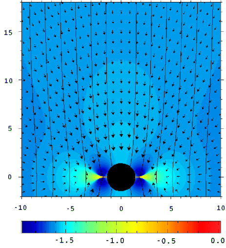
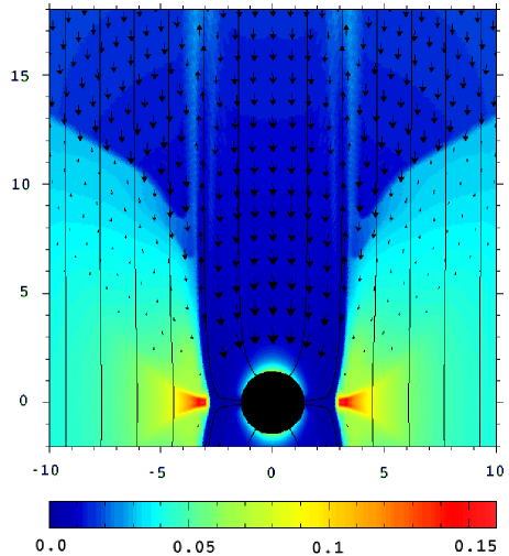
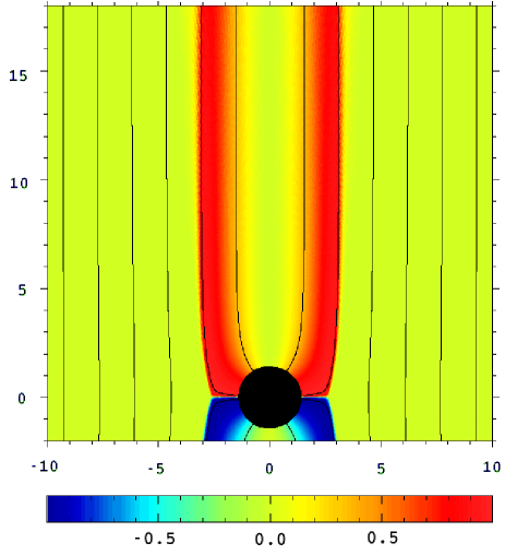
In the initial phase our numerical solution is indeed very similar to the one described in Koide [Koide 2003]. Plasma mainly slides along the magnetic field lines towards the equatorial plane where it passes through an accretion shock and forms an equatorial disc (see fig.1). The magnetic field lines are also pulled towards the black hole. Further away from the hole this seems to be mainly due the velocity field of the initial solution as the subsequent increase of the magnetic pressure in the central region quickly halts this motion and the magnetic field lines of these distant regions eventually straighten up (see fig.4). However, near the horizon this pulling is certainly caused by the hole as the field lines never straighten up there. Since similar effect is also observed in simulations of inertia-free magnetospheres [Komissarov 2004a] it cannot not be explained simply by dragging of the magnetic field lines along with the accreted plasma and has to have a more general cause. In any case, these findings are in strong contrast with the exclusion of magnetic flux by rotating black holes found in axisymmetric vacuum solutions [Wald 1974, Bicak & Janis 1985]. Those vacuum solutions were used in the past to argue low efficiency of the BZ mechanism in the case of rapidly rotating black holes. Our results shows that this argument is incorrect and vacuum solutions have to be used with more caution.
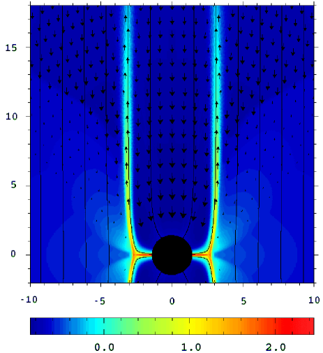
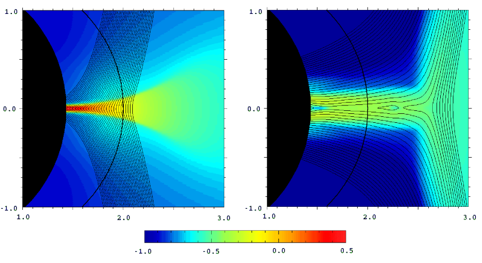
The left panel of figure 2 shows the inner region of our solution at in more detail. The colour image describes the distribution of the covariant time component of plasma’s four-velocity, , whereas the solid lines show the magnetic flux surfaces (the lines of poloidal magnetic field). For a free particle gives its specific energy at infinity. Since the hydrodynamic part of energy at infinity has the volume density
| (13) |
it can only be negative if ; because of the pressure contribution the region of negative hydrodynamic energy at infinity is somewhat narrower than the region of positive . What is even more important is that the flux of hydrodynamic energy at infinity
| (14) |
has the opposite direction to the flow velocity , as required in the MHD Penrose process, if and only if is positive. Figure 2 shows that well in agreement with findings of [Koide et al.2002, Koide 2003] the inner part of the ergospheric disc does indeed have positive during the initial phase. Moreover, the magnetic field has a very similar topology too – all magnetic field lines threading the ergospheric disc have a turning point in the equatorial plane and do not cross the event horizon.
The reason for developing positive looks attractively simple. Due to the inertial frames dragging, all plasma entering the black hole ergosphere is forced to rotate in the same sense as the black hole (to be more precise this is what is observed by a distant observer. In Kerr-Schild coordinates may have both signs.) As the result a differential rotation inevitably develops along the magnetic field lines penetrating the ergosphere which causes twisting of these lines. The Alfven waves generated in this manner propagate away from the ergosphere to infinity and establish an outflow of energy in the form of Poynting flux. Because of the energy conservation the ergospheric plasma reacts by moving onto orbits of lower energy. Provided this plasma remains in the space between the event horizon and the ergosphere for long enough it may indeed end up having negative energy.
In the problem under consideration the strong magnetic field keeps the plasma of the ergospheric disc from falling into the black hole and allows it to gain negative energy (see fig.2). However, such configuration cannot be sustain forever within ideal MHD. Since, the energy is constantly extracted along the field lines of the equatorial disc the energy of the disc is constantly going down and no steady-state can be reached. At some point the magnetic configuration would have to change so that all magnetic field lines entering the ergosphere also penetrate the event horizon (Another possible option could be a non-steady behaviour with magnetic field lines pulled in and out of the event horizon all the time.) As one can see in the right panel of figure 2, where we present the solution at , this is more or less what is observed in our simulations. At around the ergospheric disc is fully swallowed by the hole and a strong current sheet develops in its place. As the result, the structure of magnetic field becomes similar to that of the split-monopole model [Blandford & Znajek 1977]. This configuration persists till the very end of the simulations when the whole solution in the inner part of the spacial domain seems to reach a state of an approximate equilibrium.
In fact, one can see in fig.2 at least two magnetic islands in the equatorial current sheet. Such structure is known be quite typical for the tearing mode instability (e.g. Priest & Forbes, 2000) and was suggested in the context of black hole magnetospheres in Beskin (2003). Here, the islands are formed during slow reconnection events resulting in the gradual escape of magnetic flux from the event horizon, the inner islands disappear into the hole whereas the outer ones move away from it and supply hot plasma for a thin outflow sheath clearly seen in the temperature plot in fig.4. This evolution is indeed very slow and might be related to a somewhat excessive capture of magnetic field line during the early stages.
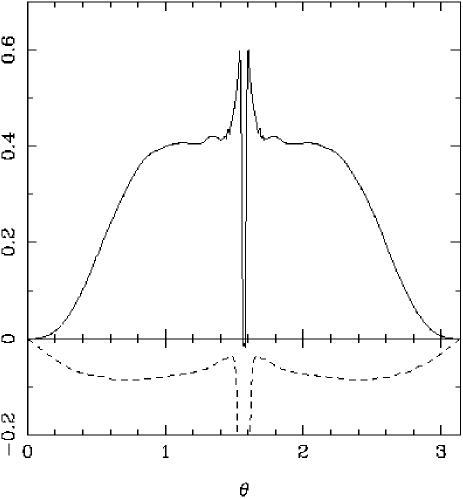
The most important feature of the solution after the restructuring of magnetic field is the total disappearance of the regions with positive (see the right panel of fig.2). Thus, the MHD Penrose process does no longer operate in the black hole ergosphere. This is confirmed in figure 3 which shows that the hydrodynamic flux of energy at infinity through the event horizon, , is everywhere negative. However, the electromagnetic flux of energy at infinity through the event horizon is positive almost everywhere with the exception of a very thin equatorial belt where it can be slightly negative (fig.3) . Thus, the pure electromagnetic Blandford-Znajek mechanism continues to operate. Moreover, the total flux of energy at infinity through the event horizon is positive and, in spite of the fact that the plasma magnetization is many orders of magnitude lower than that expected in typical astrophysical conditions, the BZ mechanism allows to extract the rotational energy of the black hole.
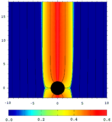
One important feature of the initial phase which has been found in the previous simulations [Koide 2003] and which persists in the longer run is the lack of any noticeable plasma outflow from the black hole. The only exception is a thin sheath of radius , most clearly seen in the top right panel of fig.4,) which is supplied with relativistically hot plasma () via the reconnection process in the ergospheric current sheet. The outflow in the sheath is rather slow with poloidal speed relative to the local FIDO never exceeding ; it is most likely driven by the gas pressure. This finding is in striking contrast with the results of MHD simulations of monopole magnetospheres of black holes which show the development of a powerful ultra-relativistic wind predominantly in the equatorial direction [Komissarov 2004b]. Being taken together, these two results suggest that divergence of magnetic field lines is a necessary condition for generating strong ultra-relativistic plasma outflows from black holes. Moreover, given the fact that the Lorentz factor of the monopole wind reaches the value of in the equatorial direction only at the distance of around r=20 (or , where , if one prefers this dimensional form) and much further away in the polar direction, one would not expected to find an MHD-driven collimated ultra-relativistic outflow at distances smaller than several tens of . Here there may be present only relativistic beams of particles accelerated by other mechanisms, e.g. electromagnetically. This makes the ongoing projects of studying the very bases (up to few tens of ) of astrophysical jets via short-wavelength VLBI observations particularly interesting [Krichbaum et al. 2004].
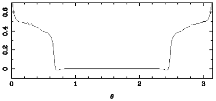
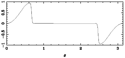
The bottom right panel of fig.4 shows the angular velocity of magnetic field lines, , normalised to the angular velocity of the black hole , where is the radius of the event horizon. In a steady state this parameter must be constant along magnetic field lines (e.g. Camenzind 1986) which is what is seen in the plot. Thus, at our solution is very close to a steady state at least for . Another interesting result seen in this plot is that , the value obtained in [Blandford & Znajek 1977] for a slowly rotating black hole with monopole magnetic field. Finally, there is a sharp transition between the “rotating column” of magnetic field lines attached to the black hole and the nonrotating ”soup” of magnetic field lines which fail to enter the ergosphere (see also fig.5). This is most likely a discontinuity somewhat smeared by numerical diffusion and perhaps by the process of reconnection in the equatorial current sheet described above.
The bottom left panel of fig.4 shows the distribution of , the covariant azimuthal component of vector introduced via
In a steady-state
where is the electric current density [Komissarov 2004a]. Thus, at the point gives us the total electric current flowing through the loop const originated from this point. In force-free steady-state solutions is also constant along magnetic field lines [Blandford & Znajek 1977, Komissarov 2004a]. This is exactly what is seen in figure 4, thus confirming that at the solution is almost force-free and very close to a steady state for . The distribution of also exhibits a discontinuity at the boundary of the “rotating column” indicating a thin current sheet of return current.
The split-monopole structure of magnetic field found in these simulations within the ergosphere is in conflict with the electrodynamic simulations where the field lines exhibit a sharp turning point in the equatorial plane [Komissarov 2004a]. There seem to be only two possible reasons for this difference. First of all, neither the inertia nor the pressure of plasma particles are accounted for in the electrodynamic model. At first glance, this does not seem to be important as even in the current MHD simulations both are small compared to the mass-energy density and pressure of magnetic field almost everywhere. But not exactly everywhere. In the equatorial current sheet the gas pressure dominates and plays a stabilizing role against otherwise quick reconnection of magnetic field lines. The second factor is the resistivity model. While the electrodynamic simulations [Komissarov 2004a] utilize the anisotropic resistivity based on the inverse Compton scattering of background photons, the only resistivity present in the MHD model is numerical. At this point we cannot exclude that explicit inclusion of physical resistivity will have a strong effect on the outcome of MHD simulations. This matter will have to be addressed in future studies.
4 Summary and Conclusions
We have carried out axisymmetric ideal MHD simulations of plasma flows in the case of a rotating black hole immersed into an initially uniform magnetic field described by the vacuum solution of Wald [Wald 1974]. Our main intention was to verify the results of previous simulations [Koide et al.2002, Koide 2003] claiming a rather significant role for the so-called MHD Penrose process of extracting the rotational energy of black holes, at least in this particular case. Our simulations show that this is true only for a short initial period during which a large fraction of magnetic field lines entering the black hole ergosphere exhibit a turning point in the equatorial plane. Eventually, those field lines are pulled into the black hole and within the ergosphere the magnetic field acquires the split-monopole structure. After this transient phase the regions of negative hydrodynamic energy at infinity are no longer present in the ergosphere and the the MHD Penrose process ceases to operate altogether.
The rotational energy yet continues to be extracted via purely electromagnetic Blandford-Znajek process [Blandford & Znajek 1977, Komissarov 2004a]. This energy extraction, however, is not followed by development of large-scale outflow from the black hole in sharp contrast with the results of previous MHD simulations for the monopole configuration of magnetic field lines [Komissarov 2004b]. The only exception is a thin current sheet located at the interface between the ”rotating column” of magnetic field lines attached to the black hole and the ”nonrotating soup” of field lines failing to enter the black hole ergosphere. The relatively slow outflow in this ”sheath” is likely to be driven by gas pressure and is fed by hot plasma produced during reconnection events in the equatorial current sheet. Given the results of these and other recent MHD simulations [Koide 2003, Komissarov 2004b] it seems impossible to generate via the standard MHD mechanism an outflow which becomes both ultrarelativistic and collimated already within the few first decades of the gravitational radius from a black hole. Should relativistic astrophysical jets continue to be seen at such small distances [Krichbaum et al. 2004], one will have to look for other explanations of their origin.
One of the main shortcoming of these simulations is the approximation of perfect conductivity. The only source of resistivity governing the process of magnetic reconnection in the developing current sheets is purely numerical. Future numerical models will have to include physical resistivity.
References
- [Beskin et al.1991] Beskin V.S., Istomin Y.N., Pariev V.I., 1991, Sov.Astron., 36(6), 642.
- [Beskin 2003] Beskin V.S., 2003, Phys.Uspekhi, 173, 1247.
- [Bicak & Janis 1985] Bicak J. and Janis V., 1985, MNRAS, 212, 899.
- [Blandford & Znajek 1977] Blandford R.D. and R.L. Znajek R.L., 1977, MNRAS, 179, 433.
- [Camenzind 1986] Camenzind, M., 1986, A&A, 162, 32.
- [Del Zanna et al.2003] Del Zanna L., Bucciantini N., Londrillo P., 2003, A&A, 400, 397.
- [De Villiers & Hawley 2003] De Villiers J.-P., Hawley J.F., 2003, ApJ, 589, 458.
- [De Villiers et al. 2003] De Villiers J.-P., Hawley J.F., Krolik J.H. 2003, ApJ, 599, 1238.
- [Evans & Hawley 1988] Evans C.R., Hawley J.F., 1988, ApJ, 332, 659.
- [Gammie et al.2003] Gammie C.F., McKinney J.C., Tóth G., 2003, ApJ, 589, 444.
- [Hirotani & Okamoto 1998] Hirotani K., Okamoto I., 1998, ApJ, 497, 563.
- [Koide et al.1999] Koide S., Shibata K., and Kudoh T., 1999, Ap.J., 522, 727.
- [Koide et al.2002] Koide S., Shibata K., Kudoh T., Meier D.L., 2002, Science, 295, 1688.
- [Koide 2003] Koide S., 2003, Phys.Rev.D, 67, 104010.
- [Koldoba et al.2002] Koldoba A.V., Kuznetsov O.A., Ustyugova G.V., 2002, MNRAS, 333, 932.
- [Komissarov 1999] Komissarov S.S., 1999, MNRAS, 303, 343.
- [Komissarov 2001] Komissarov S.S., 2001, MNRAS, 326, L41
- [Komissarov 2002] Komissarov S.S., 2002, MNRAS, 336, 759.
- [Komissarov 2004a] Komissarov S.S., 2004a, MNRAS, 350, 427.
- [Komissarov 2004b] Komissarov S.S., 2004b, MNRAS, 350, 1431.
- [Krichbaum et al. 2004] Krichbaum T.P. et al., 2004, astro-ph/0411487.
- [McKinney & Gammie 2004] McKinney J.C., Gammie C.F., 2004, ApJ, 611, 977.
- [Macdonald & Thorne 1982] Macdonald D.A. and K.S.Thorne K.S., 1982, MNRAS, 198, 345
- [Phinney 1982] Phinney E.S., 1983, in Ferrari A. and Pacholczyk A.G. eds, Astrophysical Jets, Reidel, Dordrecht, p.201.
- [Pons et al.1998] Pons J.A., Font J.A., Ibanez J.M., Martií J.M., Miralles J.A., 1998, A & A, 339, 638
- [Priest & Forbes2000] Priest E. and Forbes T., ”Magnetic Reconnection”, Cambridge University Press, Cambridge.
- [Punsly 2001] Punsly B., 2001, “Black Hole Gravitohydromagnetics”, Springer-Verlag, Berlin.
- [Punsly & Coroniti 1990a] Punsly B. and Coroniti F.V., 1990a, ApJ., 350, 518.
- [Takahashi et al.1990] Takahashi M., Niita S., Tatematsu Y., and Tomimatsu A., 1990, ApJ., 363, 206.
- [Thorne et al.1986] Thorne K.S., Price R.H., and Macdonald D.A., 1986, “The Membrane Paradigm”, Yale Univ.Press, New Haven.
- [Wald 1974] Wald R.M., 1974, Phys.Rev D, 10(6), 1680.