On Star Formation and the Non-Existence of Dark Galaxies

Abstract

We investigate whether a baryonic dark galaxy or ‘galaxy without stars’ could persist indefinitely in the local universe, while remaining stable against star formation. To this end, a simple model has been constructed to determine the equilibrium distribution and composition of a gaseous protogalactic disk. Specifically, we determine the amount of gas that will transit to a Toomre unstable cold phase via the H₂ cooling channel in the presence of a UV—X-ray cosmic background radiation field.

All but one of the models are predicted to become unstable to star formation: we find that, in the absence of an internal radiation field, the majority of gas will become Toomre unstable in all putative dark galaxies with baryonic masses greater than $10^{9}$ M_⊙, and in at least half of those greater than $10^{6}$ M_⊙. Moreover, we find that all our model objects would be detectable via HI line emission, even in the case that star formation is potentially avoided. These results are consistent with the non-detection of isolated extragalactic HI clouds with no optical counterpart (galaxies without stars) by the HI Parkes All-Sky Survey.

Additionally, where star formation is predicted to occur, we determine the minimum interstellar radiation field required to restore gravothermal stability, which we then relate to a minimum global star formation rate. This leads to the prediction of a previously undocumented relation between HI mass and star formation rate that is observed for a wide variety of dwarf galaxies in the HI mass range $10^{8}$—10¹⁰ M_⊙. The existence of such a relation strongly supports the notion that the well observed population of dwarf galaxies represent the minimum rates of self-regulating star formation in the universe.

1. Introduction

There has been long-standing speculation that optically selected galaxy surveys might be missing a population of very low surface brightness (LSB) objects (Disney, 1976; Disney & Phillipps, 1987). It has recently become possible to address this question observationally: the HI Parkes All-Sky Survey (HIPASS) has now mapped the entire Southern sky at $\sim$ 21 cm. Since the HIPASS catalogue (Meyer et al., 2004) represents an optically unbiased sample of neutral, atomic hydrogen (HI) in the local ($z\lesssim 0.04$) universe, it is ideal for the detection of HI-rich, baryonic dark galaxies; ‘galaxies without stars’.

The result of the HIPASS search for dark galaxies is emphatic and surprising. With few possible exceptions [e.g. Kilborn et al. (2000); Ryder et al. (2001); see also Minchin et al. (2005)], no isolated, extragalactic HI clouds were discovered for which an optical counterpart could not be identified (Doyle et al., 2005); it seems there are no dark galaxies.

Prior to HIPASS, the discovery of a number of ‘dim’ galaxies — “galaxies where luminous matter is only a minor component of the total galaxy mass” (Carignan & Freeman, 1988) — had led to the expectation that star formation (SF) might be suppressed completely within some galaxies. The first such examples were dwarf irregular galaxies with extended HI envelopes; DDO 154 serves as the archetype of this class of gas-rich LSB dwarfs (Krumm & Burstein, 1984). At the other end of the mass scale, the serendipitous discovery of Malin 1 (Bothun et al., 1987; Impey & Bothun, 1989), a very massive, HI-dominated LSB disk galaxy, provided an example of the class of “crouching giants” predicted by Disney (1976).

A common feature of Malin 1 and DDO 154 is their high HI mass:light ratios: $M_{\mathrm{H{I}}}/L_{B}\sim 5$ [compared to $M_{\mathrm{H{I}}}/L_{B}\sim 0.1$—1 for ‘normal’ HI-detected LSB galaxies (Fisher & Tully, 1975; Waugh et al., 2002)]. In addition to the observational problem of determining their abundance — which HIPASS has begun to address — galaxies like DDO 154 and Malin 1 pose the following theoretical problem: “Why was there so little gas processed into stars” in these systems (Carignan & Beaulieu, 1989)?

Are these objects exceptional in the way in which they are presently forming stars? How far might this ‘dim’ population extend toward complete darkness? And if dark galaxies can exist, is there some mechanism to prevent their detection by HIPASS?

In this paper, we consider the viability of dark galaxies in the local universe; that is whether a dark galaxy, having formed, can remain dark, or whether it will inevitably ‘light up’. A simple model has been developed for the distribution and composition of primordial gas in a protogalactic disk that is in chemo-dynamical equilibrium, in the presence of a photodestructive and photoheating UV—X-ray cosmic background radiation (CBR) field. The specific goal is to determine where gravothermal instability (and hence SF) is initiated through the H₂ cooling channel. Additionally, where H₂ cooling cannot be checked by the CBR alone, we place a lower bound on the global star formation rate (SFR) in these objects by determining the additional interstellar radiation field (ISRF) required to restore thermal balance.

The discussion proceeds as follows. First, an overview of the argument is provided in §2, as well as physical motivation for our model for a protogalaxy. In §3, the link between H₂ cooling and Toomre instability is discussed, and we advance our specific criterion for SF. We provide a technical discussion of the processes by which we determine the gas distribution and composition in §4 and §5, respectively. The second calculation, in which we estimate the global SFR, is then described in §6. After a discussion of fiducial parameter choices in §7, the results of our modelling procedure are given in §8, and discussed in §9. A summary of the salient and novel aspects of this work can be found in §10.

2. Overview and
Supporting Calculations

2.1. Overview of the Argument

Our primary goal is to determine whether a putative dark galaxy is gravothermally stable in its long time/steady state configuration. Where this is the case, it is conceivable that such an object (assuming that it can form) might remain dark indefinitely; otherwise, from this point, if not well before, the galaxy will inevitably ‘light up’.

Whereas rotational support stabilises against the collapse of larger-scale density fluctuations, small-scale fluctuations can only be stabilised by thermal pressure (see §3). Once the galaxy formation process is complete, the level of rotational support becomes fixed; stability is then principally determined by temperature, $T$. In particular, as will be shown in §3, most low-mass protogalactic disks are stable at $T=10^{4}$ K, while essentially all will become unstable if they are able to cool to $T\sim 300$ K.

The final temperature of the gas depends on its composition. Internal cooling of the gas proceeds by radiative de-excitation of collisionally excited atoms/molecules. Whereas HI cooling processes rapidly become inefficient (in the sense that the timescale for cooling becomes greater than the age of the universe) as collisional excitation ceases below $\sim 10^{4}$ K, H₂ cooling remains efficient above $\sim$ 300 K. The key to initiating gravothermal instability and SF in low mass disks is therefore efficient H₂ cooling; conversely, the prevention of SF requires the prevention of H₂ cooling.

Within this paradigm, SF is thus a process that must be prevented, rather than initiated: a source of dissociating radiation is required to prevent the partial conversion of HI to H₂. Within the model, the CBR is the agent for dissociation, as well as the source of heating that opposes H₂ cooling. SF is deemed to be preventable wherever the rate of photoheating due to the CBR exceeds the rate of H₂ cooling within the gas; otherwise SF is inevitable.

We thus reduce the problem of determining the in/stability of the protogalactic disk to determining the in/efficiency of H₂ cooling: we assume that gravothermal stability implies and is implied by thermal balance at $T\sim 10^{4}$ K. (We will be able to explicitly check the converse assumption — that thermal instability at $T=10^{4}$ K implies cooling to Toomre unstable temperatures — in §9.2.) Because we are interested primarily in the situation of permanent gravothermal stability, we first assume that the gaseous disk is in dynamical and chemical equilibrium at $T=10^{4}$ K; ie. a long-time configuration at the end of HI-dominated thermal evolution.

This configuration represents the long-time state of a galaxy that has managed, for whatever reason, to avoid SF, since the gas is Toomre stable so long as $T\gtrsim 10^{4}$ K; if, in this configuration, the gas cannot initiate H₂ cooling, this model therefore represents the final state of a galaxy without stars. Conversely, where H₂ cooling is inescapable, the result will be thermal, chemical, and dynamical instabilities, leading necessarily to gravothermal collapse and SF.

In other words, following authors like Corbelli & Salpeter (1995), Haiman, Thoul & Loeb (1996), Oh & Haiman (2002), and Schaye (2004), we link SF to the existence of a cold phase within the gas, and examine under what conditions the transition to the cold phase is initiated. [See, too, Elmegreen & Parravano (1994), but also Young et al. (2003).] Note that turbulent effects, which can both initiate and prevent SF, are neglected; all discussion of this point is deferred until §9.1. We have thus constructed a static problem — we make no attempt to track the evolution of the gas at any stage.

Wherever possible, our assumptions have been tailored to minimise the rates of both H₂ production and H₂ cooling, so as to make SF as difficult as possible. We thus place a firm lower limit on the mass of gas that can exist in a steady state without undergoing any SF.

Where we find that SF cannot be prevented by the action of the CBR, we perform a second calculation to place a lower limit on the expected SFR. This is done by introducing a diffuse ISRF as a second source of photoheating and photodissociation. Specifically, we determine the minimum ISRF intensity required to maintain thermal balance at $T=10^{4}$ K, and so restore gravothermal stability. With some simple assumptions (see §6), this ISRF can then be related to a minimum global SFR within the model galaxy.

2.2. The Back of the Envelope Calculation

The CBR can act to check H₂ cooling in two ways: by direct photodestruction of H₂  and by overwhelming any H₂ cooling with photoheating. The cloud’s only defence is self-shielding; ie. absorption of enough of the CBR by the outermost gas to shield inner regions from its influence.

The action of the CBR is thus to prevent SF in a shielding ‘skin’ that covers both faces of a protogalactic disk, in a manner analogous to photodissociation regions around UV sources in our own galaxy (Hollenbach & Tielens, 1999); SF is only possible in the self-shielded centre. The thickness of this skin can be characterised by the critical surface density of gas, $\Sigma_{\mathrm{crit}}$, below which the CBR is able to keep the gas completely photodissociated.

We obtain a first estimate for $\Sigma_{\mathrm{crit}}$ by noting that for the CBR to prevent the production of H₂, the total rate of photodestruction in a column (which is just the flux of photodestructive photons) must exceed the total recombination rate; viz.:

$$\frac{J_{\nu}}{h\nu}~{}\Delta\nu\gtrsim\dot{n}~{}Z_{d}~{}.$$ (1)

Here, the flux of destructive photons is approximately the product of the number of photons at the threshold frequency, $J_{\nu}/h\nu$ (where $J_{\nu}$ is the CBR flux at the threshold frequency $\nu$), and the frequency interval over which photodestructive absorption can occur, $\Delta\nu$. Similarly, the recombination rate in the column is approximately the product of the recombination rate per unit volume, $\dot{n}$, and some characteristic column height, $Z_{d}$.

With the approximations $\Sigma\approx\rho_{0}Z_{d}$ (where $\rho_{0}$ is, for now, a characteristic density), and $\dot{n}\approx\alpha x_{i}x_{j}\rho_{0}^{2}/\mu^{2}$ ($\alpha$ is the rate coefficient of the reaction between species $i$ and $j$ that replenishes the cloud’s H₂, $x_{i}$ is the relative abundance of species $i$, and $\mu\approx 1.22m_{p}$ is the mean molecular mass of particles in the gas), it is possible to rewrite inequality (1) as:

$$\Sigma\lesssim\left(\frac{J_{\nu}~{}\Delta\nu}{h\nu}~{}\frac{\mu^{2}}{\alpha x_{i}x_{j}}~{}\frac{\sigma^{2}}{2\pi G}\right)^{1/3}=\Sigma_{\mathrm{crit}}~{}.$$ (2)

In writing this expression, we have also made use of equation (17) to relate $\rho_{0}$ and $Z_{d}$, which introduces the gas velocity dispersion, $\sigma$.

Using equation (2), we can now obtain a quantitative estimate for $\Sigma_{\mathrm{crit}}$, assuming $T=10^{4}$ K (which fixes $\sigma$ and the value of $\alpha$), chemical equilibrium (which similarly fixes $x_{i}$ and $x_{j}$), and a putative CBR spectrum $J(\nu)$. To estimate $\Delta\nu$, we assume that H₂ shielding occurs between the Lyman-Werner and Lyman-$\alpha$ threshold energies, 11.2—13.6 eV. With these numbers, we calculate $\Sigma_{\mathrm{crit}}\approx$ 3—4 M_⊙ pc^-2, depending on the character of the CBR spectrum (see §7.3).

In reality, the CBR will produce at least two layers of skin: one in which it prevents HI production (ie. an ionised layer) and, internal to that, one in which H₂ production is prevented (ie. a neutral, atomic layer). Using the same argument as above, we find that the surface density of the ionised layer is $\approx$ 1 M_⊙ pc^-2.

We therefore expect that the CBR will completely prevent SF where the surface density of the protogalactic disk is less than several M_⊙ pc^-2. [For comparison, observations are consistent with a fixed SF threshold of $\sim 10$ M_⊙ pc^-2 (Taylor et al. 1994; see also Martin & Kennicutt 2001 and discussion in Schaye 2004).]

2.3. Characteristic Timescales

We assume chemo-dynamical equilibrium in our modelling. Thus, while our results do not rely on any particular galaxy formation scenario, they do depend on these equilibrium states being accessible to each system within its present lifetime. Our model does not apply to forming galaxies, nor does it attempt to follow the behaviour of the gas as it transits from warm to cold.

In particular, our criterion for SF implicitly assumes that enough time is available for the gas to cool from $T\sim 10^{4}$ K to $T\sim 300$ K after the onset of H₂ cooling. In the remainder of this section, we present some simple calculations in support of this assumption.

First, we can evaluate the timescale for cooling $t_{c}=\varepsilon/\dot{\varepsilon}$, where $\varepsilon\sim nkT$ is the thermal energy density ($n$ is the number density of the gas; $k$ is Boltzmann’s constant) and $\dot{\varepsilon}=\Lambda$ is the net cooling rate per unit volume. Using the rates of cooling listed in Appendix A, and assuming gas composition in chemical equilibrium at $T=10^{4}$ K (see Figure 3), we find $t_{c}\approx 1.5\times 10^{-3}~{}n^{-1}~{}t_{H}=20~{}n^{-1}$ Myr where $t_{H}\approx 13.7$ Gyr is the Hubble time and $n$ has units of cm^-3. (Close to the galactic plane, $n$ is typically in the range $10^{-2}$—$10^{1}$ cm^-3; see Figure 4.)

Under these conditions, the HI and H₂ cooling rates are approximately equal. In contrast, the same composition at 8000 K leads to cooling times for HI and H₂ cooling of $2.3~{}n^{-1}~{}t_{H}$ and 15 $n^{-1}$ Myr, respectively: H₂ cooling remains efficient well below the point at which HI-driven thermal evolution effectively ceases.

As we argue in §5.3, in gas near thermal equilibrium, the H₂ abundance will always approach equilibrium from above; in this case the equilibrium value therefore provides a lower limit to the actual H₂ abundance. For an H₂ abundance ten times greater than the equilibrium value, $x_{\mathrm{H}_{2}}\sim 10^{-3}$, the cooling time at $T=10^{4}$ K is reduced by a factor of 30 to $\sim 0.67n^{-1}$ Myr. Among tidal dwarf galaxies, the only observed population of presently forming galaxies, the H₂ abundance is typically as high as $x_{\mathrm{H}_{2}}\sim 0.20$ (Braine et al., 2001); the cooling time in this case is reduced to just $\sim 10^{-3}~{}n^{-1}$ Myr.

Next, we can make a rough estimate for the time needed to produce such an overabundance, $t_{\mathrm{H}_{2}}=x_{\mathrm{H}_{2}}/\dot{x}_{\mathrm{H}_{2}}$. Again assuming equilibrium abundances at 10⁴ K, and using the rate for the dominant H₂ production process (Reaction 12 in Appendix A), $\dot{x}_{\mathrm{H}_{2}}\approx 2\times 10^{-17}~{}n^{2}$ s^-1, we find $t_{\mathrm{H}_{2}}\approx 1.6~{}n^{-1}$ Myr to reach $x_{\mathrm{H}_{2}}=10^{-3}$. This value is of the same order of magnitude as if we were to take a semi-empirical rate for H₂ production on dust grains at $T\lesssim 10^{3}$ K (two-body H₂ production becomes inefficient at these temperatures), $\dot{x}_{\mathrm{H}_{2}}\sim 10^{-17}~{}n^{2}~{}\mathrm{s}^{-1}$ (Hollenbach & Tielens, 1999).

Thus, as equilibrium at 10⁴ K is disturbed, we have $t_{\mathrm{H}_{2}}<t_{c}$, and $x_{\mathrm{H}_{2}}$ increases above the equilibrium value; $t_{c}$ is accordingly diminished. At the same time, $t_{\mathrm{H}_{2}}$ increases as the temperature falls, until $t_{c}\ll t_{\mathrm{H}_{2}}$. At this point two-body chemical evolution effectively ceases, leaving a ‘freeze-out’ abundance of H₂: time-integrated studies of shock-heated (ie. $T>10^{4}$ K, $x_{\mathrm{e}^{-}}\approx 1$) gas cooling catastrophically below 10⁴ K (Shapiro & Kang, 1987; Oh & Haiman, 2002) find that $x_{\mathrm{H}_{2}}$ asymptotes to a ‘universal’ freeze-out abundance of order $10^{-3}$ at $T\sim 4000$ K. With the provision that this freeze-out H₂ abundance can survive photodissociation (see §9.2) from this point on, the gas continues to cool until $t_{c}>t_{\mathrm{H}}$ at $T\lesssim 300$ K.

Once the warm ($T\sim 10^{4}$ K) gas initiates H₂ cooling, it will therefore transit to a cold ($T\sim 300$ K) state in $\lesssim 20~{}n^{-1}$ Myr. This should be compared to the characteristic timescale for the first stage of SF, the free-fall time for a collapsing cloud, $t_{f}=(3\pi/16G\overline{\rho})^{1/2}$ $\sim 52~{}n^{-1/2}$ Myr. Where H₂ cooling occurs, the cloud will therefore cool on a timescale at least a few times faster than the collapse timescale; depending on the actual H₂ abundance, the factor is more likely $\gtrsim 30$.

3. The Model — I
The Criterion for Star Formation

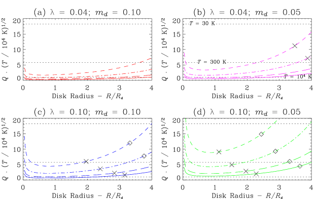
Figure 1.— Toomre profiles $Q(R)$ for various parameter sets. Panels (a) through (d) show the effect of different choices for the spin parameter, $\lambda$, and the disk mass fraction, $m_{d}$ (see §7 for a detailed description); each panel differs in only one parameter from those adjacent to it. Within each panel, profiles are shown for virial masses of $1\times 10^{8}$ M_⊙ (short-dashed line), $1\times 10^{9}$ M_⊙ (dot-dashed), $1\times 10^{10}$ M_⊙ (long-dashed), and $5\times 10^{10}$ M_⊙ (solid). The Toomre parameter is temperature dependent: within each panel, dotted lines show where the Toomre threshold ($Q=1$) would lie if the gas were at temperatures of $10^{4}$ K (bottom), 300 K (middle), and 30 K (top). Disks are unstable below the Toomre threshold. To illustrate the relationship between Toomre stability and self-shielding, we also show the radius within which the gas is self-shielding (see §8) for two different CBR spectral indices, $\eta=0.7$ (diamonds) and 2.0 (crosses).

The standard criterion for the gravothermal stability of a rotating disk, the Toomre criterion (Toomre, 1964), can be obtained from the dispersion relation for an axisymmetric density perturbation (ie. a sound wave) with wavelength $\ell$ and frequency $\omega$ [§6.2.3 of Binney & Tremaine (1987)]:

$$\omega^{2}=\kappa^{2}-2\pi G~{}\Sigma~{}\frac{2\pi}{\ell}+\left(\frac{2\pi}{\ell}\right)^{2}c_{s}^{2}~{}.$$ (3)

Here, $\kappa(R)$ is the epicyclic frequency of the orbit, and $c_{s}(T)$ is the sound speed within the gas. Since the general waveform’s time evolution is like $e^{-i\omega t}$, stability requires that $\omega^{2}>0$, and hence:

$$\left(\frac{c_{s}\kappa}{\pi G\Sigma}\right)^{2}\equiv Q^{2}\geq 1~{}.$$ (4)

This is the Toomre stability criterion, written in terms of the Toomre parameter, $Q$.

In order to determine the range of stable $\ell$s, we combine equation (3) with the condition $\omega^{2}>0$ to obtain:

$$\left(\frac{c_{s}\kappa}{\pi G\Sigma}\right)^{2}>4\left(\frac{\ell}{\ell_{\mathrm{crit}}}-\frac{\ell^{2}}{\ell_{\mathrm{crit}}^{2}}\right)~{},$$ (5)

where the left-hand side is now recognisable as $Q^{2}$. Since $Q^{2}\geq 0$, stability is assured for:

$$\ell>\ell_{\mathrm{crit}}\equiv\frac{4\pi^{2}G\Sigma}{\kappa^{2}}~{}.$$ (6)

Also, for $\ell^{2}\ll\ell_{\mathrm{crit}}^{2}$, inequality (5) reduces to:

$$\ell\lesssim\frac{c_{s}^{2}}{G\Sigma}~{},$$ (7)

which is just the Jeans criterion for the gravothermal stability of a thin disk (see also Schaye 2004). These two cases can be interpreted as the zero pressure and zero rotation limits, respectively. Large perturbations are stabilised by the effects of rotation (inequality 6), while small perturbations are stabilised by internal pressure (inequality 7).

Once the disk and halo have settled into dynamical equilibrium, all gross dynamical quantities (e.g. $\varrho_{h}$, $\Sigma$, $V$, $\kappa$) become fixed. The only variable quantity in inequality (4) that can influence $Q$ is then the sound speed, $c_{s}=(kT/\mu)^{1/2}$. The amount of the disk that is unstable therefore depends strongly on $T$. This is illustrated in Figure 1, which shows profiles of $Q(R)$ for the various parameter sets that we will consider, and the regions in which these disks would be unstable at temperatures of 10⁴ K, 300 K, and 30 K.

As mentioned in §2, for low mass disks, thermal stability at 10⁴ K implies and is implied by gravothermal stability; conversely, low mass disks only become Toomre unstable at temperatures that are only accessible via the H₂ cooling channel. Once H₂ cooling is initiated, the gas makes a rapid transition to a cold phase with $T\lesssim 300$ K (Norman & Spaans, 1997), in which case it is virtually guaranteed (at least for $M_{200}\gtrsim 10^{9}$ M_⊙) to be Toomre unstable. For these reasons, we use the H₂ cooling rate of the gas — in chemical equilibrium and at $T=10^{4}$ K — in conjunction with the Toomre criterion for gravothermal instability to define our criterion for SF.

Specifically, at a given point, star formation is deemed to occur wherever the H₂ cooling rate exceeds the total rate of photoheating, provided that the gas be Toomre unstable at $T\geq 300$ K. Figure 1 illustrates the relation between these two criteria: gravothermally unstable regions lie below the Toomre threshold; we also show the radius within which the gas is self-shielding.

4. The Model — II
The Distribution of Matter

In the next three sections, we provide a detailed, technical discussion of our three-step modelling procedure. The means by which we determine the distribution of matter in the protogalactic disk is described in this section. We discuss the solution for the equilibrium chemical composition of the gas in §5, and the calculation of the global minimum SFR is discussed in §6. A reader wishing to avoid such a technical discussion may choose to skip to §7.

The solution for the volume distribution of the gas involves two separate calculations. First, the analytic model of Mo, Mao & White (1998; hereafter MMW) is used to determine the radial distribution of matter in the model protogalaxies. The MMW model has been shown to predict some global characteristics (e.g. size distribution, velocity profiles, Tully-Fisher relation) of nearby disk galaxies and damped Lyman-$\alpha$ systems, based on more or less generic predictions of $N$-body cosmological simulations (MMW). Secondly, once the radial mass distribution is known, the vertical distribution of mass in the disk is determined using an extension of the formalism of Bahcall (1984) and Dove & Thronson (1993). These two solution processes are described in §4.1 and §4.2, respectively.

In this section, and throughout the rest of this work, the symbols $R$ and $Z$ are used to represent the (cylindrical) galactocentric radius and the vertical distance from the midplane, respectively; the lowercase $r$ is reserved for spherical coordinates.

4.1. The MMW Solution for the
Radial Mass Distribution of a Protogalactic Disk

The MMW model operates in the ‘adiabatic limit’, in which the galaxy formation process conserves an ‘adiabatic invariant’ (Barnes & White, 1984). The final configuration is thus made independent of the assembly process, making it possible, for a known initial mass distribution, to determine the final configuration, provided the form of the final disk mass distribution is specified.

Following MMW, the dark and baryonic matter are assumed to follow the same initial mass distribution; specifically, the fitting formula proposed by Navarro, Frenk & White (1997; hereafter NFW):

$$\rho_{h}(r)=\frac{\rho_{\mathrm{crit}}~{}\delta_{c}}{{r}/{r_{h}}~{}(1+{r}/{r_{h}})^{2}}~{},$$ (8)

which has been shown to describe equilibrated halos in $\Lambda$CDM cosmological simulations.

The halo scale length, $r_{h}$, is defined in relation to the quantity $r_{200}$, which is chosen such that the mean density within a sphere centred on the halo and with radius $r_{200}$ is 200 times the critical density for closure, $\rho_{\mathrm{crit}}(z)=3H^{2}(z)/8\pi G$; ie.:

$$M_{200}\equiv M(r_{200})=200~{}\rho_{\mathrm{crit}}~{}\frac{4}{3}\pi~{}r_{200}^{3}~{}.$$ (9)

Numerical experiments show $r_{200}$ to approximately demarcate between regions in which material is still in-falling, and those in which material tends towards equilibrated (radial) orbits (Cole & Lacey, 1996); $r_{200}$ and $M_{200}$ are therefore referred to as the virial radius and mass, respectively. [See Bullock et al. (2001b) for a more detailed discussion of the relation between $r_{200}$/$M_{200}$ and the virial radius/mass.] The precise relation between $r_{200}$ and $r_{h}$ is set by the concentration parameter, $c=r_{200}/r_{h}$. The normalisation factor $\delta_{c}$ in equation (8) is defined as:

$$\delta_{c}\equiv\frac{200}{3}~{}c^{3}\left(\ln(1+c)-\frac{c}{1+c}\right)^{-1}~{}.$$ (10)

Secondly, motivated by the observed distribution of light in nearby galaxies (Freeman, 1970), the assembled gaseous disk is assumed to have an exponential surface density profile, $\Sigma(R)$:

$$\Sigma(R)=\frac{m_{d}~{}M_{200}}{2\pi~{}R_{d}^{2}}~{}e^{-{R}/{R_{d}}}~{},$$ (11)

where the normalisation factor is chosen so that the total disk mass is a parametric fraction, $m_{d}$, of the total dark-plus-baryonic mass. Thus, for a given $M_{200}$ and $m_{d}$, $\Sigma(R)$ is completely specified by a scale length, $R_{d}$.

The iterative MMW solution for $R_{d}$ relates the total energy of the pre-assembly halo, $E$, to the angular momentum of the assembled disk, $J_{d}$, using the definition of the spin parameter, $\lambda$:

$$\lambda^{2}\equiv\frac{J^{2}~{}|E|}{G^{2}~{}M_{200}^{5}}~{},$$ (12)

where $J_{d}=j_{d}J$ is a parametric fraction, $j_{d}$, of the total angular momentum of the pre-assembly, dark-plus-baryonic matter halo, $J$. The final result is the following expression for $R_{d}$ (MMW):

$$R_{d}=\left(2~{}f_{c}\right)^{-0.5}~{}f_{R}~{}\frac{j_{d}~{}\lambda}{m_{d}}~{}r_{200}~{},$$ (13)

where $f_{c}(c)$ and $f_{R}(\lambda,c,m_{d},j_{d})$ are dimensionless factors of order unity, dependent on the exact shape of the initial and final mass distributions, respectively. Wherever directly comparable, our results are indistinguishable from those of MMW and of Schaye (2004).

Figure 2.— Mass distribution cross-sections for $M_{200}=10^{9}$ M_⊙, illustrating the importance of the quantity $\xi$. Contours are of constant density, in units of m_p cm^-3. Each panel is 8$R_{d}$ on a side. The disk scale height $Z_{d}(R)$ is shown by the long-dashed line; profiles are computed out to 4$Z_{d}$. Models where $\xi$ is computed as described in §4.2 are shown on the right of each frame. For comparison, models with a Spitzer (1942) sech² profile are shown on the left.

4.2. The Vertical Mass Distribution
of the Assembled Disk

Once $\Sigma(R)$ is known, at a fixed $R$, the vertical density profile for the disk gas, $\rho_{d}(R,Z)$ is governed by two equations — the Poisson equation:

$$\frac{1}{R}\frac{\partial}{\partial R}\left[R~{}\nabla\Phi_{R}\right]+\frac{\partial^{2}\Phi}{\partial Z^{2}}=4\pi G~{}(\varrho_{h}+\rho_{d})~{},$$ (14)

and the equation of hydrostatic equilibrium (in the $Z$ direction):

$$\sigma^{2}~{}\frac{\partial\rho_{d}}{\partial Z}+\rho_{d}~{}\frac{\partial\Phi}{\partial Z}=0$$ (15)

In these equations, $\Phi(R,Z)$ is the gravitational potential, $\Phi_{R}(R,Z)$ is the radial component of the potential, $\varrho_{h}(r)$ is the density of the dark matter halo (determined numerically as in Appendix B), and $\sigma$ is the (thermal) gas velocity dispersion. Since the gas is assumed to be isothermal, $\sigma$ is taken to be constant throughout the disk.

Using the equation of hydrostatic equilibrium is equivalent to using the first moment in $\overline{v_{Z}}$ of the collisionless Boltzmann equation, with the velocity dispersion tensor, $\sigma_{ij}^{2}$ (see, e.g., §4 of Binney & Tremaine, 1987), set to $\delta_{ij}\sigma^{2}$. In the context of non-interacting stellar dynamics (cf. an equilibrated gas), this assumption would introduce an error of order $(Z\,Z_{d}/R\,R_{d})$ (Bahcall, 1984).

The disk is assumed to be in centrifugal balance in the $R$ direction, and particles to travel stable, circular orbits; viz. $\nabla\Phi_{R}=V^{2}/R$, where $V(R)$ is the orbital velocity of the gas at a radius $R$. With this substitution in equation (14), these two equations can be combined by differentiating equation (15) with respect to $Z$, to give (Bahcall, 1984; Dove & Thronson, 1993):

$$\left(\frac{1}{\rho_{d}}~{}\frac{\partial\rho_{d}}{\partial Z}\right)^{2}- \frac{1}{\rho_{d}}~{}\frac{\partial^{2}\rho_{d}}{\partial Z^{2}}$$

$$=\frac{4\pi G}{\sigma^{2}}~{}\rho_{d}\ + \frac{4\pi G}{\sigma^{2}}~{}\left(\varrho_{h}-\frac{1}{4\pi G~{}R}~{}\frac{\partial V^{2}}{\partial R}\right)~{}.$$ (16)

Following Bahcall (1984) and Dove & Thronson (1993), equation (16) is made dimensionless by defining a scale height for the disk $Z_{d}(R)$:

$$Z_{d}(R)\equiv\left(\frac{\sigma^{2}}{2\pi G~{}\rho_{0}(R)}\right)^{{1}/{2}}~{},$$ (17)

where $\rho_{0}(R)=\rho_{d}(R,~{}0)$ is the volume density of the disk gas on the plane, at a distance $R$ from the galactic centre. [Note that $Z_{d}$ is twice the exponential scale height (Bahcall, 1984).] This leads (again, for a fixed $R$) to an ordinary differential equation for the dimensionless density $y(x)=\rho_{d}(R,Z)/\rho_{0}(R)$, where $x=Z/Z_{d}$:

$$\frac{d^{2}y}{dx^{2}}=\frac{1}{y}\left(\frac{dy}{dx}\right)^{2}-2~{}y^{2}-2~{}\xi(R,Z)~{}y~{},$$ (18)

subject to the boundary conditions:

$$y(x=0)=1~{}~{}~{}~{}~{}~{}\mathrm{and}~{}~{}~{}~{}~{}~{}\frac{dy}{dx}\Big{|}_{x=0}=0~{}.$$ (19)

It is worth making a few comments here about the quantity $\xi$ in equation (18), which is defined as:

$$\xi(R,Z)\equiv\frac{1}{4\pi G\rho_{0}}\left(4\pi G\varrho_{h}(r)-\frac{1}{R}\frac{\partial V^{2}(R)}{\partial R}\right)~{},$$ (20)

but which can be rewritten in a more convenient form (Appendix B). If $\xi$ is neglected altogether, then equation (18) is analytic, yielding $y(x)=\mathrm{sech}^{2}~{}x$ (Spitzer, 1942). This formalism was first derived in the context of stellar dynamics close to the galactic plane and at modest distances from the galactic centre, in which case both $V$ and $\varrho_{h}$ vary slowly across the volume of interest. Authors therefore typically neglect the $\partial V^{2}/\partial R$ term and treat $\varrho_{h}$ as constant (e.g. Maloney 1993; Dove & Shull 1994).

This work, however, considers lower mass galaxies with manifestly non-flat rotation curves. Moreover, we are interested primarily in the outermost gas, since this is where the effects of the CBR are greatest; this is also where the effect of a non-zero $\xi$ is most pronounced. It is therefore inappropriate to adopt these standard approximations here. The effect of a non-zero $\xi$ is illustrated in Figure 2, which shows several model gas distributions as well as the equivalent distribution assuming $y=\mathrm{sech}^{2}~{}x$.

In summary, the modelling procedure is as follows: $y(x)$ is determined by numerical integration of equation (18); $\rho_{0}$ is then fixed with reference to the definition of $\Sigma(R)$, viz.:

$$\rho_{0}=\frac{2\pi G~{}\Sigma^{2}(R)}{\sigma^{2}~{}\left(2\int_{0}^{\infty}dx~{}y(R,x)\right)^{2}}~{}.$$ (21)

The presence of $\rho_{0}$ in the definition of $\xi$, as well as the implicit dependence of $\xi$ on $Z$, make it necessary to solve for $y(x)$ iteratively: a trial value of $\rho_{0}$ is used to determine the value of $\xi$ in the integration of equation (18); the value of the integral is then used in equation (21) to obtain the next $\rho_{0}$. This process rarely requires more than several iterations for convergence.

5. The Model — III
The Chemical Composition
of the Gas and the CBR

Once the distribution of the disk gas is known, we determine its equilibrium chemical structure. Nine chemical species are identified within the gas, interacting via 21 collisional and nine photodestructive processes, as outlined in §5.1. The gas is subject to a UV—X-ray CBR field; we describe the CBR parameterisation, including gas self-shielding, in §5.2. The solution for the equilibrium chemical composition of the gas is discussed in §5.3.

5.1. Chemical Species and Processes

Following Haiman, Thoul & Loeb (1996; hereafter HTL) and Abel et al. (1997), we distinguish nine chemical species within the gas: $\mathrm{H}^{0}$, $\mathrm{H}^{-}$, $\mathrm{H}^{+}$, $\mathrm{H}_{2}^{0}$, $\mathrm{H}_{2}^{+}$, $\mathrm{He}^{0}$, $\mathrm{He}^{+}$, $\mathrm{He}^{++}$, and $\mathrm{e}^{-}$, assuming a (primordial) helium mass fraction of 0.24. These chemical species are allowed to interact via the 21 collisional processes identified by HTL. In addition, the nine photoionisation and photodissociation processes listed in Abel et al. (1997) are included. For ionisation of $\mathrm{He}^{0}$ and $\mathrm{H}_{2}^{0}$, the more recent cross-sections given by Yan, Sadeghpour & Dalgarno (1998) are employed. These expressions give much lower cross-sections at high energies than those used by Abel et al. (1997), which reduces the rate of heating in marginally shielded areas, but increases the penetration depth. The rate coefficients and cross-sections for all of these processes are listed in full in Appendix A.

We completely neglect the effects of any dust or metals present in the gas, even though the IGM is expected to have seen considerable enrichment (Aguirre et al., 2001; Schaye el al., 2000). Metals can make a significant contribution to the cooling rate within the self-shielded region (Galli & Palla, 1998; Katz, Weinberg & Hernquist, 1996); moreover, both dust and metals act as sites for H₂ production. These effects only become dominant, however, once two-body collisional production of H₂ becomes inefficient, well below the assumed temperature of $10^{4}$ K (Buch & Zhang, 1991; Galli & Palla, 1998). Further, both dust and metals can absorb UV CBR radiation, so contributing to the level of self-shielding within the cloud. The neglect of dust and metals therefore minimises the predicted level of H₂ production and cooling.

For each individual chemical species, an expression can be written for the net rate of production/consumption in terms of the number densities of all nine species. It is most convenient and instructive to cast these expressions in terms of the relative chemical abundances, $x_{i}=n_{i}/n_{\mathrm{H}}$, where $n_{i}$ is the number density of species $i$, and $n_{\mathrm{H}}$ is the number density of hydrogen nuclei, viz.:

$$\frac{dx_{i}}{n_{\mathrm{H}}~{}dt}=\sum_{p}{\bigg{[}}\sum_{q}{\bigg{(}}b_{pq}^{(i)}~{}\alpha_{p,q}~{}x_{p}~{}x_{q}{\bigg{)}}+~{}d_{p}^{(i)}~{}\frac{\Gamma_{p}}{n_{\mathrm{H}}}~{}x_{p}~{}{\bigg{]}}~{}.$$ (22)

Here, $\alpha_{p,q}$ is the temperature dependent rate coefficient for the reaction between $p$ and $q$, $\Gamma_{p}$ is the rate of photoionisation/photodissociation of $p$, and $b_{pq}^{(i)}$, $d_{p}^{(i)}$ = 0, $\pm$1, or $\pm$2, depending on the number of $i$ particles produced/consumed in the reaction. Note that in the high density/zero radiation limit, the equilibrium abundances are independent of density; they are determined by the temperature dependent $\alpha$s alone. Equation (22) encapsulates a particularly ‘stiff’ set of nine highly nonlinear coupled differential equations for the chemical composition of the gas at a fixed point (HTL).

5.2. The Photodestructive Effects of the CBR

We consider the CBR in the range 13.6 eV $\leq h\nu\leq$ 40 keV (ie. 912 Å $\geq\lambda\geq 0.31$ Å— we find that photoionisation of He and He⁺ by soft X-rays is important in H₂ production, as well as being a significant photoheating mechanism.) Within this range, the CBR spectrum, $J_{\mathrm{CBR}}(\nu)$, is described using a simple power law, characterised by its spectral index, $\eta$, and a normalisation constant, $J_{21}$, chosen such that:

$$J_{\mathrm{CBR}}(\nu,\,R,\,Z)=J_{21}~{}\left(\frac{\nu}{\nu_{\mathrm{H{I}}}}\right)^{-\eta}~{}e^{-\tau(\nu;R,Z)}$$

$$\times 10^{-21}\mathrm{~{}erg^{-1}~{}s^{-1}~{}Hz^{-1}~{}cm^{-2}~{}Sr^{-1}}~{}.$$ (23)

Here, $\nu_{\mathrm{H{I}}}$ is the frequency of the Lyman-$\alpha$ photon: $h\nu_{\mathrm{H{I}}}\approx 13.6$ eV. This parameterisation is the simplest possible; to assess its relevance, we direct the reader to the compendium of CBR observations across the whole electromagnetic spectrum provided by Henry (1999). We will trial two extreme values of $\eta$ (see §7.3), in an attempt to bracket the real situation.

The frequency dependent optical depth, $\tau$, defined as:

$$\tau(\nu;\,R,\,Z)=\sum_{i}\bigg{[}a_{i}(\nu)\int^{\infty}_{Z}dZ^{\prime}~{}n_{i}(R,Z^{\prime})\bigg{]}~{},$$ (24)

is used to modulate the CBR spectrum as it penetrates into the cloud, so mimicking radiative transfer. Here, $a_{i}(\nu)$ is the frequency dependent cross-section for photodestruction of species $i$, as given in Appendix A. Note that this treatment of radiative transfer is ‘one way’ — no attempt has been made to account for radiation that crosses the midplane — leading to a very minor underestimation of the photoheating rate close to the plane.

We have made three substantial omissions in writing equations (23) and (24). First, any extinction of the CBR due to the presence of dust or metals has been neglected. Secondly, secondary ionisations by energetic electrons from X-ray ionisations are ignored. While these ionisations have no effect on the heating rate, the enhanced electron abundance would increase the H₂ production rate (and the total rate of cooling); the omission of secondary ionisations will therefore again lead to a lower limit on the shielded fraction. Thirdly, and most importantly, diffuse radiation produced by the gas itself has been ignored; that is, any photons (re-)radiated by the gas are assumed to be free to escape unhindered. This assumption is justified for the optically-thin outermost gas; its validity within the self-shielded region is certainly problematic, but a detailed treatment of radiative diffusion through the cloud would be dependent on both the thermal and dynamic evolution of the disk during its formation. As has been stated, this is beyond the scope of the present undertaking.

For each photoreaction except Solomon photodissociation of H₂ (see below), the photodissociation/photoionisation rate, $\Gamma_{i}$, is then given by:

$$\Gamma_{i}=2\pi\int_{\nu_{i}}^{\infty}d\nu~{}\frac{J(\nu)}{h\nu}~{}a_{i}(\nu)~{},$$ (25)

where $\nu_{i}$ is the threshold energy for dissociation of species $i$, and the factor of 2$\pi$ arises from integration over all angles of incidence onto the flat disk.

Photodissociation of H₂ occurs primarily in the Lyman-Werner bands (11.26—13.6 eV) via the two-step Solomon process (Stecher & Williams, 1967):

$$\mathrm{H}^{0}\ +h\nu\rightarrow\ \mathrm{H}_{2}^{*}\rightarrow\ 2\mathrm{H}^{0}~{}.$$ (26)

This process is harder to deal with than other photoprocesses, since the structure of the molecular energy levels (and so the cross-section for photodestruction) is so much more complex. Moreover, Doppler broadening causes individual lines to overlap. Following Abel et al. (1997), absorption is therefore restricted to the Lyman band (12.24—13.51 eV); the CBR spectrum is treated as flat in this narrow range. Thus, rather than explicitly considering H₂ dissociating photons longward of 912 Å, the H₂ photodissociation rate is determined with reference to the mean number of photons near 1000 Å. The penetration probability formalism of de Jong, Dalgarno & Boland (1980), which modulates the unextinguished CBR field with a shielding factor, $\beta$, is used to simulate H₂ self-shielding, including the effects of Doppler broadening; the adopted expression for $\beta(\tau_{\mathrm{H}_{2}})$ is given in Appendix A.

5.3. Chemical Composition in Equilibrium

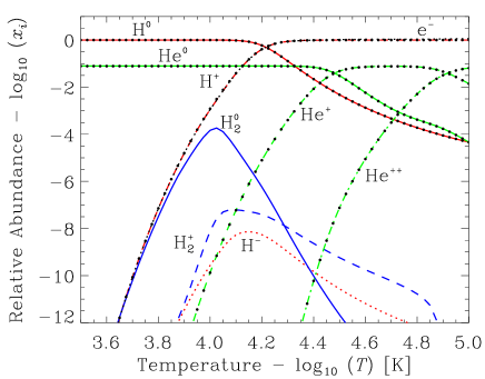
Figure 3.— Equilibrium abundances of nine chemical species in the absence of any photodestruction. Chemical species are as labelled. The points show the equilibrium solutions for the reduced set of equations in which $\mathrm{H}^{-}$, $\mathrm{H}_{2}^{0}$, and $\mathrm{H}_{2}^{+}$ are omitted. All abundances are scaled relative to the total hydrogen nucleus number density, $n_{\mathrm{H}}$. Note that the electron abundance closely tracks the proton ($\mathrm{H}^{+}$) abundance. This plot is provided only as a diagnostic for our solution procedure, and should not be mistaken for actual evolutionary tracks. (see §5.3).

Once the radiation density at a given point is known (and hence the rate coefficients for the various photochemical processes), it is possible to find the equilibrium chemical composition at that point by solving the system of equations represented by equation (22), with the time derivatives on the left-hand side set to zero. We do this using a modified Netwon-Raphson algorithm (§9 of Press et al. 1992), where we compute the Jacobi matrix analytically. For $dx_{i}/dt=0$, only six of the nine equations remain independent; it is also necessary to ensure that the total number of hydrogen nuclei, helium nuclei, and electrons are conserved separately (Katz, Weinberg & Hernquist, 1996).

As a diagnostic for the solution procedure only, Figure 3 shows the equilibrium chemical composition (in the absence of photodestruction) as a function of temperature. In this plot, the lines show our steady-state solutions for the full set of equations encapsulated by equation (22); for comparison, the points show algebraic solutions for a reduced system of six equations obtained by omitting $\mathrm{H}^{-}$, $\mathrm{H}_{2}^{0}$, and $\mathrm{H}_{2}^{+}$. Note that these results differ significantly from those in the directly comparable Figure 2 of HTL, which were obtained by direct integration of equation (22) until apparent convergence. In particular, our predicted $\mathrm{H}_{2}^{0}$ abundance is one to two orders of magnitude lower than that of HTL, depending on the reaction rate expressions used (see Appendix A). The disagreement arises from the fact that the results shown in HTL had not yet fully converged (Zoltán Haiman, private communication — note that this does not affect the conclusions of HTL), as can be readily verified by direct substitution.

It should also be noted that, contrary to Haiman, Rees & Loeb (1996), assuming chemical equilibrium is expected to lead to a lower limit on the actual H₂ abundance at $T=10^{4}$ K, and by extension on the H₂ cooling rate. The assumed rate coefficient for H₂ production is temperature independent, while that for consumption decreases with temperature; thus, the effect of a small decrease in temperature is an increase in the net rate of H₂ production [see, e.g., Figure 4 of Abel et al. (1997)]. The net rate of H₂ production, therefore, can only go to zero if the H₂ abundance is dropping (or if the gas temperature is rising). The H₂ abundance in an equilibrating gas will therefore always reach equilibrium from above. (For a time-evolved demonstration of this point, see Figure 4 of Haiman, Abel and Rees 2000.)

Moreover, the situation of chemical equilibrium for H₂ is physically improbable for temperatures between $\sim 10^{3}$—$10^{4}$ K, because in the absence of a source of photoheating, the gas will be thermally unstable; gas is far more likely to cool past these temperatures without equilibrating. In this sense, we emphasise the limited physical relevance of Figure 3, which is provided only as a diagnostic, and refer the reader to plots of nonequilibrium abundances in cooling and collapsing gas clouds like those found in Figures 3—5 of Oh & Haiman (2002), Figure 3 of Abel et al. (1997), or Figure 6 of Shapiro & Kang (1987).

Figure 4.— Contours of $u_{d}$, shown in cross section. $u_{d}$ is the minimum ISRF energy density (at 1000 Å) required for thermal balance, determined as per §6. Contours are shown (in units of the Habing flux) for example model ($\lambda,~{}m_{d}$) = (0.04, 0.05); clockwise from top-left are models with $M_{200}=5\times 10^{10},~{}10^{10},~{}10^{9}$, and $10^{8}$ M_⊙. Note the different ranges of the vertical axes in the upper ($R_{d}$) and lower ($4R_{d}$) panels. We only solve for $u_{d}$ at radii where the gas is Toomre unstable at $T\geq 300$ K (see Figure 1). Overlaid are contours of $n_{\mathrm{H}}$ (dotted lines), in units of cm^-3.

6. The Model — IV
The Minimum SFR

At each point where H₂ cooling is found to be sufficient to initiate gravothermal instability, we introduce an additional internal radiation field and determine the minimum ISRF required to preserve thermal balance at $10^{4}$ K; it is then possible to relate this ISRF to a minimum global SFR, ${\cal R}_{\mathrm{min}}$. In other words, we solve for the minimum ISRF-regulated SFR within the cloud.

This is done by including a tenth equation in the system of equations described in §5.3, requiring that the collisional H₂ cooling rate ($\Lambda_{\mathrm{H}_{2}}$, given in Appendix A) be balanced by the net rate of photoheating, viz.:

$$\sum_{i}\zeta_{i}-\Lambda_{\mathrm{H}_{2}}=0~{}.$$ (27)

Here, $\zeta_{i}$ is the rate of photoheating due to absorption by species $i$, which (for all processes except Solomon dissociation of H₂— see Appendix A) is given by:

$$\zeta_{i}=n_{i}~{}\int_{\nu_{i}}^{\infty}d\nu~{}(h\nu-h\nu_{i})~{}\frac{J(\nu)}{h\nu}~{}a_{i}(\nu)~{},$$ (28)

where the radiation flux $J=J_{\mathrm{CBR}}+cu_{d}$ now has two components. The first is due to the CBR, where $J_{\mathrm{CBR}}$ is defined by equation (23); the second is the new diffuse ISRF, characterised by the diffuse radiation energy density, $u_{d}$. Note that we use this same $J$ in equation (25), so that the ISRF maintains thermal balance by some combination of photoheating and H₂ photodissociation.

The spectral shape of $u_{d}$ is fixed with reference to the stellar population modelling utility Starburst99 (Leitherer et al., 1999), which gives the SED for continuous star-formation, $L_{99}(\nu)$, with units of erg s^-1 Hz^-1 (1 M_⊙ yr${}^{-1})^{-1}$. We adopt a standard SF scenario, which assumes a Salpeter IMF over a mass range of 1—100 M_⊙, and a metallicity of 0.020 (Z_⊙); our results are not strongly dependent on the choice of metallicity. Over the spectral range of interest, this SED converges after $\lesssim 10$ Myr (a few times the lifetime of O—B stars); we use this converged SED. It should be noted that the Starburst99 SED only extends to 100 Å; since self-shielding against the diffuse ISRF is ignored, this will lead to only a minor underestimate of the rate of HeI ionisation, and so the rate of heating.

To convert this luminosity to a radiation density, it is necessary to make an estimate of the mean lifetime of each photon, $\tilde{t}_{\nu}$, which is done with reference to the mean free path of a photon with energy $h\nu$, $\ell_{\nu}\equiv(na_{\nu})^{-1}=\tilde{t}_{\nu}c$. With these substitutions, $u_{d}$ can be written:

$$u_{d}(\nu)={\cal U}~{}L_{99}(\nu)~{}\left(c\sum_{i}n_{i}a_{i}(\nu)\right)^{-1}~{}.$$ (29)

While the spectral shape of $u_{d}$ is given by $L_{99}$, its intensity is thus characterised by a scale factor, ${\cal U}$, which has the units of a SFR per unit volume.

${\cal U}$ is thus taken as the tenth unknown in a system of ten equations, representing the minimum SFR (per unit volume, and assuming chemical equilibrium) required to produce a sufficient ISRF to maintain thermal balance at $T=10^{4}$ K, and so restore gravothermal balance. Note that ${\cal U}$ gives the SFR required to ensure the stability of the volume $dV$, not the SFR within $dV$. Figure 4 shows the resultant ISRF field in cross-section for several exemplary models. A global SFR, ${\cal R}_{\mathrm{min}}$, is then found by integrating ${\cal U}=d{\cal R}_{\mathrm{min}}/dV$ over the whole disk.

Clearly, this is not a solution for the exact problem. That said, ${\cal R}_{\mathrm{min}}$ is expected to provide a reasonable estimate for the minimum SFR in the cloud, since ‘maximum damage’ has been allowed; photons are delivered directly to wherever they are required. Under these conditions, so long as the actual SFR exceeds ${\cal R}_{\mathrm{min}}$, the non-star-forming remainder of the disk will remain stable; otherwise, some part of the disk will become unstable and the SFR will increase as a result.

7. The Model — V
Choice of Parameters

The model now outlined consists of three components described by nine parameters. In this section, the fiducial values adopted for these parameters are discussed.

Cosmology enters our calculations via $\rho_{\mathrm{crit}}$, which is used to determine $r_{200}$ for a given $M_{200}$ (see equation 9); we adopt the now standard WMAP cosmology (Bennett et al., 2003; Spergel et al., 2003). Further, model disks are assumed to form at zero redshift. Since $\rho_{\mathrm{crit}}$ decreases with decreasing redshift, $r_{200}$, and hence $R_{d}$, will be greater for smaller disk formation redshifts (see equation 9); at a fixed $R/R_{d}$, this minimises $\rho_{d}$ and so self-shielding and H₂ production, in keeping with the ethos of the model.

7.1. The Progenitor Halo: $M_{200}$, $c$, $\lambda$

The maximum virial mass considered is $M_{200}=5\times 10^{11}$ M_⊙, typical of a nearby LSB galaxy. The minimum mass, $M_{200}\approx 10^{8}$ M_⊙, is set by the form of the analytic model: below this limit, the solution process for $Z_{d}$ and $\rho_{0}$ fails to converge at $R\sim R_{d}$. Mathematically, the long, slow rise of the rotation curve for lower mass galaxies makes $\xi$ a large negative number at these radii, which eventually drives the vertical density profile, $y(x)$, to increase with distance off the plane (see equation 20). In this unphysical case, we truncate the integration, and treat the stationary point as a sharp boundary. It may be that lower mass halos do not form exponential disks.

The concentration parameter, $c$, is chosen using a simple scaling relation drawn from Figure 6 of Navarro, Frenk & White (1996):

$$c=7.5\left(\frac{M_{200}}{M_{*}}\right)^{-1/9}~{},$$ (30)

where $M_{*}$ is the (cosmology dependent) ‘nonlinear’ mass, as defined in that work.

Numerical experiments show that the spin distribution in hierarchical clustering scenarios is well described by a ‘log-normal’ distribution centred at $\lambda_{0}=0.04$, and with width $\delta\lambda=0.5$ (Warren et al., 1992; Bullock et al., 2001a). Two values for the spin parameter, $\lambda$, are adopted to sample this distribution: a ‘typical’ value of 0.04, and a ‘high’ value of 0.10. These values approximately correspond to the 50 and 90 percent points of the expected distribution (see also MMW).

7.2. The Disk: $m_{d}$, $j_{d}$, $\sigma$, $T$

Based solely on the WMAP cosmology (Spergel et al., 2003), baryons are expected to make up 16 percent (by mass) of all matter. However, not all of the baryonic material initially within an overdense region will ultimately settle into the disk. Moreover, of the mass that does collect at the centre of the potential well, some fraction may be lost, e.g. through evaporation after reionisation (Shaviv & Dekel, 2003). Two fiducial values for the disk mass fraction are therefore adopted, $m_{d}=0.05$ and 0.10 (see also MMW).

Assuming that the halo’s angular momentum originates from tidal torquing, it is natural to assume that both the dark and baryonic components obtain the same specific angular momentum (Fall & Efstathiou, 1980); thus, at the time of virialisation, $m_{d}=j_{d}$. While $N$-body and hydrodynamic simulations predict that $j_{d}/m_{d}$ is significantly less than unity for assembled disks, (Navarro & White, 1994; Navarro & Steinmetz, 1997), the MMW model requires that $j_{d}/m_{d}$ be close to unity in order to produce disk sizes and properties that are in agreement with observations. Accordingly, we assume $j_{d}=m_{d}$ for the assembled disk.

The velocity dispersion, $\sigma$, is assumed to be constant, with the value of $8.2$ km s^-1; this corresponds to the thermal velocity dispersion at $T=10^{4}$ K. Our chosen value is larger than the canonical value of 6 km s^-1, which, using a recalibrated Toomre criterion ($Q<2$), has been shown to predict the location of star formation thresholds in around 2/3 of nearby spiral galaxies (Kennicutt, 1989; Martin & Kennicutt, 2001). However, Schaye (2004) has recently suggested that this agreement is largely coincidental: for typical HSB disk galaxies only, the point where the disk is Toomre unstable assuming $c_{s}=\sigma=6$ km s^-1 fortuitously coincides with where the transition to the cold phase becomes possible.

7.3. The CBR Field: $J_{21}$, $\eta$

The CBR parameters are fixed using the value of the low-redshift HI photoionisation rate, $\Gamma_{\mathrm{H{I}}}$, obtained by Scott et al. (2002). They give a best fit value of $\Gamma_{\mathrm{H{I}}}=2.0^{+9.0}_{-1.4}\times 10^{-13}$ s^-1 for $z<1$, where $\Gamma_{\mathrm{H{I}}}$ is related to the UV—X-ray CBR spectrum by:

$$\Gamma_{\mathrm{H{I}}}=4\pi~{}\int_{\nu_{\mathrm{H{I}}}}^{\infty}d\nu~{}\frac{J_{\mathrm{CBR}}(\nu)}{h\nu}~{}a_{\mathrm{H{I}}}(\nu)~{}.$$ (31)

Here, $a_{\mathrm{H{I}}}$ is the known cross-section of HI (see Appendix A). For a power law spectrum, this integral can be performed analytically, which makes it possible to fix the normalisation constant $J_{21}$ for a given spectral index $\eta$.

We consider two fiducial values for $\eta$. The first, $\eta=2$, mimics a typical quasar spectrum (Scott et al., 2002); the second, $\eta=0.7$ is chosen to match cosmological simulations of the Lyman-$\alpha$ forest and the observed X-ray CBR up to 40 keV (Haiman, Rees & Loeb, 1996). Using the Scott et al. (2002) value for $\Gamma_{\mathrm{H{I}}}$, these two choices correspond to values for $J_{21}$ of 0.091 and 0.071, respectively.

8. Results

We determine the amount and distribution of gas (assuming chemo-dynamical equilibrium at $T=10^{4}$ K) that is subject to H₂ cooling in the presence of the CBR. Where the cooling rate due to H₂ processes exceeds the total rate of heating due to the CBR (ie.  where the gas is thermally unstable at 10⁴ K) the gas is deemed ‘shielded’. If this gas is also Toomre unstable at $T\geq 300$ K (ie. if it will be gravothermally unstable in the cold phase), then it is deemed ‘unstable’; this gas is then prone to star formation. Additionally, by determining the ISRF intensity required to restore thermal balance at $T=10^{4}$ K at each ‘unstable’ point (so restoring the situation of gravothermal stability), we estimate the minimum global SFR for each model.

A few trial models have been recalculated with greater precision to ensure that numerical effects do not significantly alter our results; our principal results, shown in Figures 6 and 7, are convergent to better than 1 percent.

8.1. Localised Properties of Model Disks

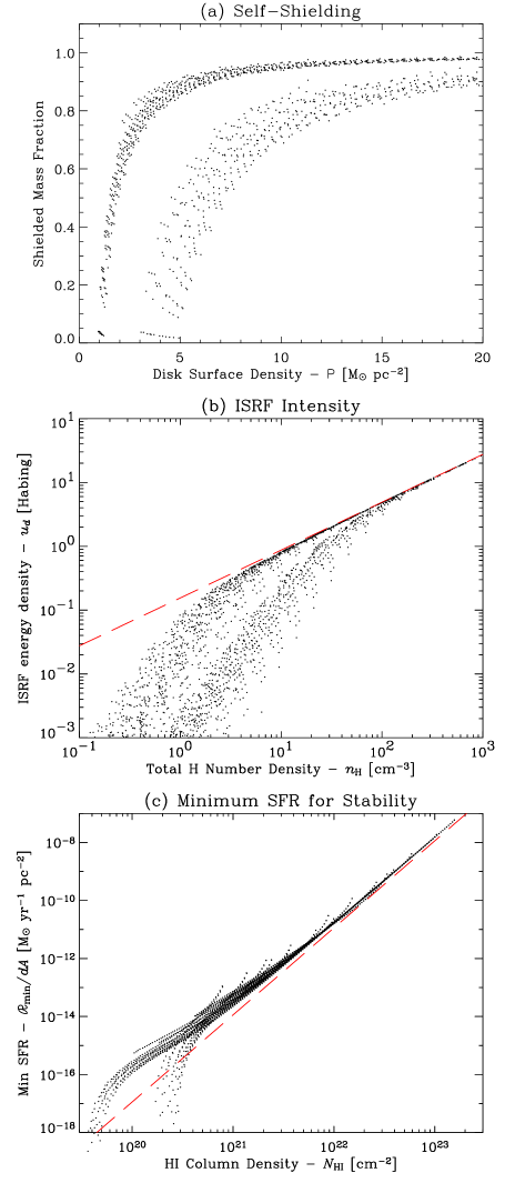
Figure 5.— Local scaling relations arising in the model: (a) The fraction (by mass) of gas that is shielded from the CBR as a function of surface density; (b) the minimum ISRF intensity required to maintain thermal balance at $10^{4}$ K as a function of density; (c) the minimum SFR required to maintain thermal balance as a function of HI column density. Representative points are drawn from each of the 32 parameter sets we have modelled. Within each panel, the two distinct curves correspond to $\eta=2.0$ (upper curves) and $\eta=0.7$ (lower curves). Panel (c) should not be interpreted in terms of a Schmidt relation. The SFR plotted in panel (c) is the SFR required elsewhere in the cloud to prevent SF in a column of density $N_{\mathrm{H{I}}}$; it is not the SFR expected in that column.

In Figure 5, we present some of the ‘local’ scaling relations that arise within the models. Within each panel, the two distinct curves in regions of marginal shielding correspond to the two choices of CBR spectral index: the upper curve to $\eta=2.0$, the lower one to $\eta=0.7$.

First, in panel (a), the mass fraction of shielded gas is plotted as a function of surface density. These results are in good agreement with the first estimate made in §2.2. A universal vertical density profile would ensure that all columns with the same $\Sigma$ would be self-similar; the scatter in this plot — particularly in the $\eta=2.0$ case, which has a higher proportional X-ray flux — therefore demonstrates of the importance of detailed modelling of the vertical gas distribution. Within the scatter, the trend with increasing mass is right to left; more massive disks are better able to self-shield.

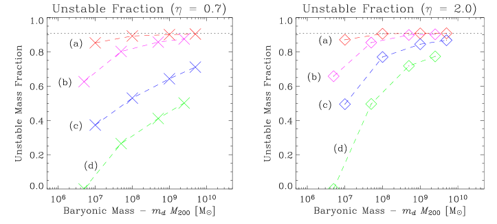
Figure 6.— The fractional mass that is unstable to SF in the absence of an internal ISRF. The left panel shows models with $\eta=0.7$; the right shows $\eta=2.0$. Within each panel, from top to bottom, parameter sets are ($\lambda,~{}m_{d}$) = (0.04, 0.10), (0.04, 0.05), (0.10, 0.10), (0.10, 0.05). In other words, lower spin galaxies are more unstable than higher spin; then for the same spin, a higher fractional disk mass reduces stability. Note that for an exponential disk, only $\sim 90$ percent of the mass resides within $4R_{d}$; this point is shown by the dotted line. Even for the ‘worst case’ CBR, the majority of baryonic matter is unstable to SF in at least 50 percent of all galaxies with baryonic masses greater than a few times $10^{6}$ M_⊙; the same is true for all galaxies with baryonic masses greater than $\sim 10^{9}$ M_⊙.

In panel (b), the minimum ISRF intensity required to maintain thermal balance at $10^{4}$ K, $u_{d}$, is plotted as a function of gas density. The ISRF is presented in units of the Habing ‘flux’ (the observed local ISRF energy density at 1000 Å), $g=40\times 10^{-18}$ erg Å^-1 cm${}^{-3}=1.33\times 10^{-29}$ erg Hz^-1 cm^-3 (Habing, 1968). Within the self-shielded region, $u_{d}=0.16~{}n_{\mathrm{H}}^{0.75}~{}g$; this relation has been overplotted.

Finally, in panel (c), the minimum SFR (per unit projected area) required to preserve thermal balance, ${\cal R}_{\mathrm{min}}/dA$, is plotted as a function of HI column density. Again, within the self-shielded region, the curves converge towards a power law: ${\cal R}_{\mathrm{min}}/dA\approx 1.1\times 10^{-14}~{}(N_{\mathrm{H{I}}}/10^{21}$ cm${}^{-2})^{3}=2.2\times 10^{-17}~{}\Sigma_{\mathrm{H{I}}}^{3}$. The results plotted in this panel agree very well with those of Corbelli, Galli & Palla (1997). Note that surrounding the completely self-shielded region is one in which ${\cal R}_{\mathrm{min}}/dA$ exceeds this power law: in this region, the CBR actually aids SF, as the increased electron abundance due to X-ray ionisation of HeI enhances H₂ production.

Since thermal balance within the self-shielded region is achieved primarily through photodissociation of H₂ (rather than heating by the CBR), the results of the ISRF calculation are sensitive to the H₂ photodissociative flux alone. The predictions for $u_{d}$ are therefore robust, in that they should not be sensitive to the assumed ISRF spectral shape, or to the exact distribution of the gas. However, the link between $u_{d}$ and ${\cal R}_{\mathrm{min}}/dV$ is more tenuous, since the exact relation depends on the extent, location, and character of SF within the cloud.

8.2. Integrated Properties of Model Disks

Figure 6 shows the fractional mass of gas available for star formation for each of the 32 parameter sets that we have modelled. All else being equal, high spin galaxies are less able to self-shield than those with lower spin. In the high spin case, $R_{d}$ is typically 8—10 times greater than for low spin, which reduces the surface density at a fixed $R/R_{d}$ by a factor of order 50—100.

Also, a CBR spectrum with a shallower spectral index has a greater proportional X-ray flux, and so is able to penetrate deeper into the cloud. At a fixed point, this increases the rate of photoheating; at the same time, the free electrons from helium ionisations lead to an increased H₂ production rate. Thus, in the $\eta=0.7$ case, even though the CBR aids SF near the shielding boundary, this boundary is pushed deeper within the gas.

Recalling that the adopted values for $\lambda$ represent the 50 and 90 percent points of the expected distribution, the majority of the disk is predicted to be unstable to SF in at least 50 percent of putative dark galaxies with baryonic masses greater than $5\times 10^{6}$ M_⊙. For baryonic masses greater than $10^{8}$ M_⊙, the majority of mass is unstable in as much as 90 percent of all protogalaxies, depending on the distribution of $m_{d}$ and the true CBR spectrum.

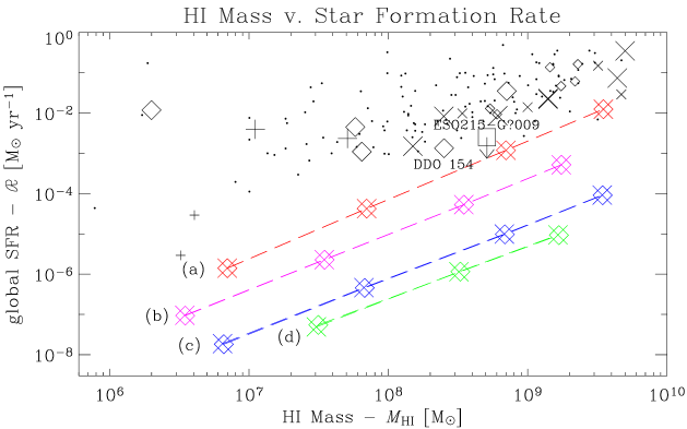
Figure 7.— Minimum SFR required for stability, ${\cal R}_{\mathrm{min}}$, plotted against HI mass, $M_{\mathrm{H{I}}}$. As in Figure 6, like models are connected with a dashed line to guide the eye: from top to bottom, models are ($\lambda,~{}m_{d}$) = (0.04, 0.10), (0.04, 0.05), (0.10, 0.10), (0.10, 0.05); $\eta=0.7$ (2.0) models are plotted with crosses (diamonds). Note that the top and bottom pairs of lines represent the 50 and 90 percent points of the expected spin distribution, respectively, and that we have deliberately attempted to place a firm lower bound on ${\cal R}_{\mathrm{min}}$. For comparison, observed values of $M_{\mathrm{H{I}}}$ and SFR for a variety of dwarf galaxies are overplotted, including: ‘nearby’ (large pluses) and ‘distant’ (small pluses) dwarfs from Hunter, Elmegreen & Baker (1998); ‘low’ SFR (small crosses) and ‘high’ SFR (large crosses) nearby HI-bright dwarfs from Young et al. (2003); ‘LSB’ (small diamonds) and ‘normal’ (large diamonds) dwarfs from van Zee et al. (1997); 121 members of a sample of irregular galaxies (points), spanning a large range in galactic parameters, from Hunter & Elmegreen (2004); and the extremely HI-rich dwarf ESO215-G?009 (large square) (Warren, Jerjen & Koribalski, 2004). See §9.4 for a discussion of the significance of this relation.

This result is directly contrary to that of Verde, Oh & Jimenez (2002), who have predicted that all disks in halos with $M_{200}<10^{9}$ M_⊙ should remain dark. However, these authors have assumed a constant $c_{s}=\sigma$ = 6 km s^-1 when calculating the Toomre parameter, which implies $T\approx 8500$ K; in the context of this model, this is tantamount to ignoring H₂ cooling.

The predicted global minimum SFR within the putative dark galaxies, ${\cal R}_{\mathrm{min}}$, is plotted in Figure 7, as a function of the HI mass, $M_{\mathrm{H{I}}}$; in all cases, $M_{\mathrm{H{I}}}/m_{d}M_{200}$ is between 0.56 and 0.70. For comparison, some observed values of $M_{\mathrm{H{I}}}$ and SFR for actual dwarf galaxies have been overplotted. We have included: a sample of six “relatively nearby” ($D\lesssim 15$ Mpc) Im and seven “more distant” ($30\lesssim D\lesssim 100$ Mpc) Im and Sm galaxies from Hunter, Elmegreen & Baker (1998); four HI-bright nearby galaxies, two each with “low” ($<10^{-4}$ M_⊙ yr^-1) and “high” ($>10^{-4}$ M_⊙ yr^-1) SFRs, from Young et al. (2003); seven LSB dwarf galaxies and four “normal” dwarfs from van Zee et al. (1997); 121 irregular galaxies from the sample of Hunter & Elmegreen (2004), which span more than 8 mag in absolute magnitude and surface brightness; and ESO215-G?009, an extremely HI-rich dwarf galaxy, with the highest accurately measured HI mass:light ratio to date, $M_{\mathrm{H{I}}}/L_{B}\sim 20$ (Warren, Jerjen & Koribalski, 2004).

For each combination of $\lambda$ and $m_{d}$, ${\cal R}_{\mathrm{min}}\propto M_{\mathrm{H{I}}}^{1.4}$. We note that this relation has the same power as the empirical Schmidt SF law, SFR$/dA\propto\Sigma_{\mathrm{H{I}}}^{1.4}$ (Schmidt 1959; Kennicutt 1989, 1998; but see also Boissier et al. 2003). Moreover, even though these samples were selected to include widely disparate populations, these populations are not readily distinguished in Figure 7 for $M_{\mathrm{H{I}}}\gtrsim 10^{8}$ M_⊙, nor is the exceptional ESO215-G?009 clearly differentiated from the others.

These results are essentially independent of the CBR spectral index. For the HI fraction, which is determined principally by the outermost gas in the cloud, this is because the CBR spectrum has been normalised using $\Gamma_{\mathrm{H{I}}}$. On the other hand, ${\cal R}_{\mathrm{min}}$ is determined principally by the dense gas closest to the plane of the disk and to the centre of the galaxy, where the effect of the CBR is least. In combination with the results in Figure 6, this gives the surprising result that ${\cal R}_{\mathrm{min}}$ is essentially independent of the amount of gas that is deemed ‘unstable’; it depends on $M_{\mathrm{H{I}}}$ alone.

9. Discussion

9.1. The Effects of Substructure and Turbulence

It is difficult to be quantitative about the effect of substructure, but, qualitatively, self-shielding is increased where the surface density is enhanced. Since, to first order, the CBR prevents a skin of fixed column depth from entering the cold phase, removing matter from a marginally shielded column and adding it to a well shielded column will increase the overall shielded fraction. That is, the omission of substructure such as bars and turbulent cloudlets should again lead to an underestimate of the amount of gas prone to SF.

Wada, Meurer & Norman (2002) have shown that statistically stable turbulence, leading to a multi-phase interstellar medium, can be produced and sustained with no stellar energy input. It is conceivable that this turbulence could dominate the velocity dispersion, so providing a third mechanism for support against gravitational collapse. The turbulent velocity dispersion required to support gas at $T\sim 300$ K, however, is typically more than 15 km s^-1, whereas in the model these authors present, the turbulent velocity dispersion is only 1—5 km s^-1.

Moreover, Wada & Norman (2001) have shown that the timescale for cooling is far shorter than the several dynamical times required to establish this turbulent motion. In their model, the central gas cools within 0.1 Myr, whereas turbulent effects first become apparent only after $\sim$ 2 Myr, and stabilise after $\sim$ 10 Myr. While turbulent effects are not unexpected in these galaxies, we therefore expect them to be insufficient to stabilise the gas, and to emerge only after the first bout of star formation.

Figure 8.— Minimum temperature achieved by cooling gas, $T_{\mathrm{min}}$, plotted against the critical temperature below which the gas becomes Toomre unstable, $T_{Q}$, for representative points in regions deemed unstable. Where $T_{Q}>T_{\mathrm{min}}$, gas is able to make an evolutionary transit to a Toomre unstable cold phase, in line with the argument presented in §3. This is essentially always true.

9.2. An Important Sanity Check

The crux of our argument is the assumption that, if and when H₂ cooling is initiated, the gas will rapidly evolve into a cold phase at $T\sim 300$ K. In §2.3, we have argued that this transition will be fast in comparison to the dynamical timescale; we are now in a position to verify that this transition will, in fact, lead to Toomre instability.

Detailed integration of the coupled rate equations encapsulated by equation (22) have found that gas cooling from $T\gtrsim 10^{4}$ K to $T\lesssim 300$ K develops a non-equilibrium abundance of H₂, $x_{\mathrm{H}_{2}}\sim 10^{-3}$ (Shapiro & Kang, 1987; Susa et al., 1998; Oh & Haiman, 2002), nearly independently of the initial conditions. This occurs at $T\sim 4000$ K, when (two-body) collisional H₂ production and consumption processes become inefficient, leaving an un-replenishing ‘freeze-out’ abundance of H₂. In the presence of a photodestructive radiation field, these molecules can be quickly destroyed, preventing further cooling. Oh & Haiman (2002) have shown that, because of the scalings in the problem, the final temperature that a parcel of gas (at fixed $n$) is able to cool to depends only on the ratio $J/n$.

Oh & Haiman (2002) describe a method for estimating the minimum temperature achieved by a cooling parcel of gas, $T_{\mathrm{min}}$, by finding the temperature for which the timescales for cooling, $t_{c}$, becomes longer than that for photodissociation, $t_{d}=\Gamma_{\mathrm{H}_{2}}^{-1}$. With the approximation $\Lambda_{\mathrm{H}_{2}}\propto T^{4}$, and assuming the freeze-out abundance, $x_{\mathrm{H}_{2}}=10^{-3}$, this leads to the following expression for $T_{\mathrm{min}}$:

$$T_{\mathrm{min}}\approx 9000~{}\left(\frac{\beta~{}J_{21}}{n}\right)^{1/3}~{}{\mathrm{K}}~{}.$$ (32)

(Recall that $\beta$ is the H₂ self-shielding factor, discussed in §5.2.) It should be noted that this analysis does not include dust catalysed H₂ production at $T\lesssim 3000$ K.

In Figure 8, we plot $T_{\mathrm{min}}$ (for gas in unstable regions) as a function of the critical temperature below which the gas becomes Toomre unstable, $T_{Q}$. Points that lie above the line $T_{\mathrm{min}}=T_{Q}$ represent regions where the gas will transit to a Toomre stable cold phase, in violation of the assumption on which we base our SF criterion. There do appear to be very rare violations of this assumption, however these points are those closest to the shielding boundary (far from the midplane), in the most Toomre stable regions (far from the centre) and make an insignificant contribution to the important integrated quantities.

9.3. Implications for Star Formation

Our model argues for a subtle but significant alteration to the (often unstated) conventional wisdom concerning SF: that HI is the raw material from which stars form. Within this paradigm, HI is commonly referred to as ‘unprocessed’ gas, and it is common and reasonable to interpret the Schmidt ‘law’ as a causal relation between an amount of gas and the level of SF.

The primary role of H₂ cooling in this picture lies in the fragmentation of a collapsing gas cloud into protostellar cloudlets. We have shown, however, that H₂ can also be important in initiating the first Toomre/Jeans instability. This is particularly important in the case of low mass galaxies which would remain Toomre stable if their thermal evolution were governed by HI alone.

The importance of this slight revision lies in the interpretation of HI observations. The picture outlined above interprets HI as, in some sense, the ‘original’ state of hydrogen. In the alternate scenario, however, H₂ can be seen as a ‘default’ state for hydrogen: wherever possible, HI will always develop into H₂. Moreover, since H₂ cooling virtually guarantees Toomre instability, some external source of UV radiation is required to prevent the production of stars from within the gas by dissociating H₂ into HI. In this new paradigm, HI is thus a product of SF rather than being its primary fuel, and the Schmidt relation is symptomatic of the mode of SF.

In other words, the Schmidt relation should not be interpreted as ‘given more HI, more stars will form’, but instead as ‘more UV radiation (produced by short-lived O—B stars) is required to support a bigger HI cloud.’ [For a detailed exposition of this argument, see Allen (2002).]

This revision is not so controversial: the importance of H₂ cooling in low mass galaxy formation has been well established by works such as Peebles & Dicke (1968), Lepp & Shull (1984), Haiman, Thoul & Loeb (1996), and Kepner, Babul & Spergel (1997). Although these works are typically (but not exclusively) focused on the effect that radiative feedback from the first generation of stars has on galaxy formation, they clearly demonstrate the importance of H₂ in the global thermal and dynamic evolution of galaxies before protostellar fragmentation. Closer to home, the established physics of photodissociation regions [see Hollenbach & Tielens (1999) for a comprehensive review] demonstrate the importance of the UV ISRF in producing HI in our galaxy.

9.4. The $M_{\mathrm{H{I}}}$—SFR Relation
and DDO 154–like Galaxies

Our model predicts a hitherto undocumented relation between HI mass and SFR, which seems to hold over the range $M_{\mathrm{H{I}}}\sim 10^{8}$—$10^{10}$ M_⊙: SFR $\propto M_{\mathrm{H{I}}}^{1.4}$. Within the model, this relation is a manifestation of self-regulating SF (Lin & Murray, 1992; Omukai & Nishi, 1999), in which the ISM is kept warm and stable by a UV ISRF that is maintained by constant regeneration of O—B stars.

The slope of the relation is driven by the distribution of the densest gas in galaxy centres, since it is this gas that requires the most radiation to maintain thermal stability. The scatter is set primarily by the distribution of galactic spins, as well as variations in the relative mass of the disk in comparison to the halo, since, for a fixed mass, these determine the density near the centre.

Because the model was designed to place a lower limit on the SFR, it cannot predict the zero-point of such a relation. Within the self-shielded region, the H₂ cooling rate is typically less than 1—10 percent of the net cooling rate; a significantly higher ISRF might be required to balance these other cooling mechanisms. Moreover, if there were, for example, a systematic run with mass in the relative contribution of metal-line cooling in comparison to H₂ cooling, the inclusion of metals might alter the predicted slope of the relation. We stress that this would only be true, however, if metal-line cooling were important in initiating the transition from warm to cold.

The general agreement between the character of the predicted and observed $M_{\mathrm{H{I}}}$—SFR relations lends weight to the physical picture on which this simple model is based: the results in Figure 7 suggest that the well observed population of dwarf galaxies represent the minimum rate of ISRF-regulated SF in galaxies.

Moreover, in the range $M_{\mathrm{H{I}}}\sim 10^{8}$—$10^{10}$ M_⊙, it seems that the majority of dwarfs are forming stars in the same way: ‘extreme’ objects like DDO 154 and ESO215-G?009 are not distinguished from ‘normal’ dwarfs in the $M_{\mathrm{H{I}}}$—SFR plane. In response to the question “Why was so little gas processed into stars?”, therefore, these galaxies’ high HI mass:light ratios are not due to inefficiencies in the present mode of SF. Instead, they may be, for example, a reflection of late formation times or differing environmental effects.

9.5. The Complete Prevention of SF

Figures 6 and 7 show that SF is completely prevented in only one of the models: ($M_{200},~{}\lambda,~{}m_{d}$) = ($10^{8}$ M_⊙, 0.10, 0.05). As is apparent in Figure 1, this is due primarily to rotational support rather than an inability to self-shield: the gas is self-shielding at $R\approx$ 1 (2.5) $R_{d}$ for $\eta=0.7$ (2.0), but is never Toomre unstable at $T=300$ K. However, if the gas were able to cool to $\sim 30$ K (ie. if it could initiate metal line cooling), then up to 70 percent of the gas would become available for SF, and we would predict ${\cal R}_{\mathrm{min}}\sim 10^{-9}$ M_⊙ yr^-1.

9.6. The Detectability of Dark Galaxies

Throughout this work, since the focus has been on gravothermal stability in the absence of internal SF, it has been implicitly assumed that the gas is predominantly HI (and not HII or H₂). Clearly, a very large stellar component would be necessary to completely ionise the gas, and it has been shown that the gas becomes gravothermally unstable in the presence of small amounts of H₂. It has also been argued that, once SF begins, the ISRF will regulate the SFR by dissociating H₂ into HI.

HI is detectable by the hyperfine transition at $\sim 21$ cm, provided that the excitation temperature, $T_{\mathrm{spin}}$, exceeds the mean background radiation temperature, $T_{\mathrm{bg}}\approx 3$K. $T_{\mathrm{spin}}$ can be written (Kulkarni & Heiles, 1988):

$$T_{\mathrm{spin}}=\frac{T+y~{}T_{\mathrm{bg}}}{1+y}~{},$$ (33)

where, neglecting HI excitation by electron collisions, $y\sim(T/1000$ K) / ($n_{\mathrm{H{I}}}/0.2$ cm^-3). From Figure 5, it is apparent that $n_{\mathrm{H{I}}}$ is essentially always in the range 10^-1—10² cm^-3 within the self-shielded region, in which case $T_{\mathrm{spin}}$ = 800—9800 K. Moreover, since HI is so optically thick to Lyman-$\alpha$, even the low predicted SFRs act to thermalise $T_{\mathrm{spin}}$ via scattered Lyman-$\alpha$ photons.

Without exception, all models are thus predicted to have detectable HI emission, independently of their optical properties. Joint optical–plus–21cm surveys are therefore predicted to yield complete samples of galaxies.

10. The Existence of Dark Galaxies — Summary

We have developed a model for the long-time configuration of a baryonic dark galaxy, in order to determine whether such a galaxy, having formed, could conceivably remain dark. The model has the following features:

• The gas is in a dynamically equilibrated disk (rotationally supported in the radial direction and in hydrostatic equilibrium vertically) at the end of the galaxy formation process.

• The gas is isothermal at $T=10^{4}$ K, which represents the endpoint of its thermal evolution in the absence of H₂ cooling. Together, the assumptions listed above limit the model to considering galaxies with $M_{200}\gtrsim 10^{8}$ M_⊙.

• The gas is in chemical equilibrium, in the presence of a UV—X-ray CBR. The CBR can prevent SF by preventing the gas from undergoing a transition (driven by H₂ cooling) from a warm, largely stable phase to a cold, mostly unstable phase.

We evaluate the stability of this situation of thermal, chemical and dynamical equilibrium by determining whether or not H₂ cooling can induce gravothermal instability, and hence SF, in the face of the CBR. Additionally, wherever an ISRF is required (in addition to the CBR) to counterbalance H₂ cooling, we place an approximate lower bound on the expected SFR.

We find that, in the absence of an internal UV radiation field, gas that is sufficiently self-shielded to support an H₂ abundance as low as 10^-4 is unable to remain gravothermally stable. This statement remains true independently of any other cooling processes, including metal line cooling: so as to place a firm lower bound on the amount of gas that will become gravothermally unstable, we have ignored the significant shielding and cooling effects of dust and metals when calculating the H₂ cooling rate at 10⁴ K. Moreover, if the gas is even mildly enriched, then its final temperature drops by an order of magnitude from $\sim$ 300 K to $\sim$ 30 K (Norman & Spaans, 1997); particularly for the models most affected by the CBR, this could significantly reduce stability against SF (Figure 1).

Our conclusions can be summarised as follows:

1. The model predicts a correlation between HI mass and SFR, which is observed in a wide variety of dwarf galaxies (see Figure 7). This suggests that dwarf galaxies represent the minimum levels of ISRF-regulated SF in the universe. Further theoretical and observational studies of this relation should prove fruitful.

2. With only one exception, the modelled galaxies cannot avoid SF indefinitely, and so will develop a stellar component. Even for baryonic masses as low $5\times 10^{6}$ M_⊙, the majority of gas in greater than 50 percent of all halos is unstable to SF in the absence of an internal ISRF (Figure 6).

3. Without exception, all models would have detectable HI emission. That is, whatever dark or dim galaxies exist should be detectable in HIPASS–class surveys.

Above the detection limit of $M_{\mathrm{H{I}}}\sim 7\times 10^{6}$ M_⊙ (Meyer et al., 2004), HIPASS did not detect any extragalactic HI clouds in the Local Group that did not also have a stellar component. Similar results are available for other groups and clusters (Zwaan, 2001; Waugh et al., 2002). Within these limits, there is no reason to suspect a population of undetected baryonic dark galaxies.

We wish to thank Stuart Wyithe for many fruitful discussions in the course of this work, and Joop Schaye for his helpful and insightful responses to an early draft. We also thank the anonymous referee, whose comments led to the calculation presented in §9.2. ENT was supported by a University of Melbourne–CSIRO collaborative grant while this work was completed.

Appendix A Chemical Processes in the Disk

The full list of reactions considered in this study is given in Table A1, along with their rate coefficients. All quantities in this section are listed in cgs units. The symbol $T_{n}$ is used to denote $T^{-n}$. Note that the rate coefficient for reaction (21) has two terms; the second term arising from dielectric recombination (Cen, 1992). The rates given for reactions (16) and (17) both are valid in the low density ($n_{H}<10^{4}~{}\mathrm{cm^{-3}}$) limit.

Also note that three of the expressions given in Table 3A of Haiman, Thoul & Loeb (1996) differ from those given in the works that those authors cite. They give the exponent of $T_{3}$ in the expression for the rate coefficient of reaction (2) as 0.2; it should read -0.2 [This typographical error is not present in Haiman, Rees & Loeb (1996)]. More seriously, the multiplying factor in the expression for reaction rate (3), given as 5.57, should read 3.23. Also, the exponent of $T$ in reaction rate (6), which should be 2.17, is omitted in Haiman, Thoul & Loeb (1996). These alterations reduce the equilibrium abundances of H₂ by several orders.

#	Reaction		Rate Coefficient, $\alpha$ (cm3 s -1)	Ref.
(1)	$\mathrm{H}^{0}$+ $\mathrm{e}^{-}$$\rightarrow$	$\mathrm{H}^{+}$+ 2$\mathrm{e}^{-}$	$5.85\times 10^{-11}~{}T^{1/2}~{}e^{-157809.1/T}~{}(1+T_{5}^{1/2})^{-1}$	Cen92
(2)	$\mathrm{H}^{+}$+ $\mathrm{e}^{-}$$\rightarrow$	$\mathrm{H}^{0}$+ $h\nu$	$8.40\times 10^{-11}~{}T^{-1/2}~{}T_{3}^{-0.2}~{}(1+T_{6}^{0.7})^{-1}$	Cen92
(3)	$\mathrm{H}^{0}$+ $\mathrm{e}^{-}$$\rightarrow$	$\mathrm{H}^{-}$+ $h\nu$	$3.23\times 10^{-17}~{}T^{1/2}$	HTL96
(4)	$\mathrm{H}_{2}^{0}$+ $\mathrm{e}^{-}$$\rightarrow$	$\mathrm{H}^{-}$+ $\mathrm{H}^{0}$	$2.7\times 10^{-8}~{}T^{-3/2}~{}e^{-43000/T}$	HTL96
(5)	$\mathrm{H}^{0}$+ $\mathrm{H}^{-}$$\rightarrow$	$\mathrm{H}_{2}^{0}$+ $\mathrm{e}^{-}$	$1.3\times 10^{-9}$	Raw88
(6)	$\mathrm{H}^{0}$+ $\mathrm{H}^{-}$$\rightarrow$	2$\mathrm{H}^{0}$+ $\mathrm{e}^{-}$	$5.3\times 10^{-20}~{}T^{2.17}~{}e^{-8750/T}$	S&K87
(7)	$\mathrm{e}^{-}$+ $\mathrm{H}^{-}$$\rightarrow$	$\mathrm{H}^{0}$+ 2$\mathrm{e}^{-}$	$4\times 10^{-12}~{}T~{}e^{-8750/T}$	S&K87
(8)	$\mathrm{H}^{+}$+ $\mathrm{H}^{-}$$\rightarrow$	2$\mathrm{H}^{0}$	$7\times 10^{-7}~{}T^{-1/2}$	D&L87
(9)	$\mathrm{H}^{+}$+ $\mathrm{H}^{-}$$\rightarrow$	$\mathrm{H}_{2}^{+}$+ $\mathrm{e}^{-}$	$4\times 10^{4}~{}T^{-1.4}~{}e^{-15100/T}~{}:~{}T>10^{4}$ K
			$10^{-8}~{}T^{-0.4}~{}:~{}T\leq 10^{4}$ K	S&K87
(10)	$\mathrm{H}^{+}$+ $\mathrm{H}^{0}$$\rightarrow$	$\mathrm{H}_{2}^{+}$+ $h\nu$	$3.255\times 10^{-20}~{}T-4.152\times 10^{-25}~{}T^{2}-6.157e^{-17}~{}:~{}T>4000$ K
			$1.38\times 10^{-23}~{}T^{1.845}~{}:~{}200\leq T\leq 4000$ K	RDB93
(11)	$\mathrm{H}^{+}$+ $\mathrm{H}_{2}^{0}$$\rightarrow$	$\mathrm{H}_{2}^{+}$+ $\mathrm{H}^{0}$	$2.4\times 10^{-9}~{}e^{-21200/T}$	S&K87
(12)	$\mathrm{H}^{0}$+ $\mathrm{H}_{2}^{+}$$\rightarrow$	$\mathrm{H}_{2}^{0}$+ $\mathrm{H}^{+}$	$6.4\times 10^{-10}$	HTL96
(13)	$\mathrm{H}^{-}$+ $\mathrm{H}_{2}^{+}$$\rightarrow$	$\mathrm{H}_{2}^{0}$+ $\mathrm{H}^{0}$	$5\times 10^{-6}~{}T^{-1/2}$	D&L87
(14)	$\mathrm{e}^{-}$+ $\mathrm{H}_{2}^{+}$$\rightarrow$	2$\mathrm{H}^{0}$	$1.68\times 10^{-8}~{}(T/300)^{-0.29}$	HTL96
(15)	$\mathrm{H}_{2}^{0}$+ $\mathrm{H}^{0}$$\rightarrow$	3$\mathrm{H}^{0}$	$6.11\times 10^{-14}~{}e^{-29300/T}~{}:~{}T>7390$ K
			$2.67\times 10^{-15}~{}e^{-(6750/T)^{2}}~{}:~{}T\leq 7390$ K	L&S83
(16)	$\mathrm{H}_{2}^{0}$+ $\mathrm{H}_{2}^{0}$$\rightarrow$	$\mathrm{H}_{2}^{0}$+ 2$\mathrm{H}^{0}$	$5.22\times 10^{-14}~{}e^{32200/T}~{}:~{}T>7291$ K
			$3.17\times 10^{-15}~{}e^{-(4060/T)-(7500/T)^{2}}:T\leq 7291$ K	S&K87
(17)	$\mathrm{H}_{2}^{0}$+ $\mathrm{e}^{-}$$\rightarrow$	2$\mathrm{H}^{0}$+ $\mathrm{e}^{-}$	$4.38\times 10^{-10}~{}T^{0.35}~{}e^{-102000/T}$	S&K87
(18)	$\mathrm{He}^{0}$+ $\mathrm{e}^{-}$$\rightarrow$	$\mathrm{He}^{+}$+ 2$\mathrm{e}^{-}$	$2.38\times 10^{-11}~{}T^{1/2}~{}e^{-285335.4/T}~{}(1+T_{5}^{1/2})^{-1}$	HTL96
(19)	$\mathrm{He}^{+}$+ $\mathrm{e}^{-}$$\rightarrow$	$\mathrm{He}^{++}$+ 2$\mathrm{e}^{-}$	$5.68\times 10^{-12}~{}T^{1/2}~{}e^{-631515.0/T}~{}(1+T_{5}^{1/2})^{-1}$	Cen92
(20)	$\mathrm{He}^{+}$+ $\mathrm{e}^{-}$$\rightarrow$	$\mathrm{He}^{0}$+ $h\nu$	$1.50\times 10^{-10}~{}T^{-0.6353}$
			$~{}+~{}1.9\times 10^{-3}~{}T^{-3/2}~{}e^{-470000/T}(1+0.3e^{-94000/T})$	Cen92
(21)	$\mathrm{He}^{++}$+ $\mathrm{e}^{-}$$\rightarrow$	$\mathrm{He}^{+}$+ $h\nu$	$3.36\times 10^{-10}~{}T^{-1/2}~{}T_{3}^{-0.2}(1+T_{6}^{0.7})^{-1}$	Cen92

Table A1 — Reaction rate coefficients. The expressions given for reactions (16) and (17) are valid for $n_{H}<10^{4}~{}\mathrm{cm^{-3}}$. References: (Cen92) Cen (1992); (D&L87) Dalgarno & Lepp (1987); (HTL96) Haiman, Thoul & Loeb (1996); (L&S83) Lepp & Shull (1983); (Raw88) Rawlings (1988); (RDB93) Rawlings, Drew & Barlow (1993); (S&K87) Shapiro & Kang (1987). All coefficients are given in cgs units. Note that the rate coefficients for reactions (2), (3) and (6) given in Haiman, Thoul & Loeb (1996) disagree with those given in the works those authors cite (see text).

For photoionisation and photodissociation reactions, we employ the reaction cross-sections given by Abel et al. (1997), except for ionisation of $\mathrm{He}^{0}$ and $\mathrm{H}_{2}^{0}$, for which we use the more recent expressions given by Yan, Sadeghpour & Dalgarno (1998). The different asymptotic behaviour of the expression for $\mathrm{He}^{0}$ ionisation has a significant effect on the chemical structure of our models, but does not drastically affect our conclusions. When calculating the cross-section for H₂ ionisation, we assume all H₂ to be in the para- configuration. This is appropriate only when reactions (5) and (12) are the dominant H₂ production mechanisms; within the model these reaction rates are typically seven orders of magnitude higher than for reaction (13).

To account for self-shielding of H₂ against LW photons, including the effects of Doppler broadening and line overlap, we use the shielding factor of de Jong, Dalgarno & Boland (1980):

$$\beta(\tau)=\left(\left(\frac{\tau^{2}}{2}~{}\ln\left[\frac{\tau^{2}}{\pi}\right]\right)^{-1/2}+\left(\frac{\tilde{a}}{\tau}\right)^{1/2}\right)~{}\times\mathrm{erfc}\left[\left(\frac{\tau\tilde{a}}{\pi a_{\mathrm{H}_{2}^{0}}}\right)^{1/2}\right]~{},$$

where erfc denotes the complimentary error function, and $\tilde{a}=9.2\times 10^{-3}~{}\sigma^{-1}$ cm km s^-1 is called the Voigt parameter. Following de Jong (1977), we assume that each Solomon dissociation heats the gas by 2.5eV.

Finally, we use the lengthy expression given by Lepp & Shull (1983) for the rate of H₂ cooling, $\Lambda_{\mathrm{H}_{2}}$:

$$\Lambda_{\mathrm{H}_{2}}=\left(\frac{L_{vH}}{1+(L_{vH}/L_{vL})}+\frac{L_{rH}}{1+(L_{rH}/L_{rL})}\right)~{}n_{\mathrm{H}_{2}}~{}~{}:~{} L_{vH}=1.10\times 10^{-18}~{}e^{-6744/T}$$

$$L_{vL}=8.18\times 10^{-13}~{}\left(\alpha_{16}~{}n{{}_{\mathrm{H}^{0}}}+\alpha_{17}~{}n_{\mathrm{H}_{2}^{0}}\right)$$

$$L_{rH}=3.90\times 10^{-19}~{}e^{-6118/T}$$

$$L_{rL}=\left(1.38\times 10^{-22}~{}e^{-9243/T}\right)~{}Q_{n}$$

$$Q_{n}=1.2~{}(n{{}_{\mathrm{H}^{0}}})^{0.77}+(n_{\mathrm{H}_{2}^{0}})^{0.77}~{},$$

where each of the $L$s has units of ergs s^-1. As given here, this expression is valid only for temperatures above 4031 K. For the calculation presented in §9.2, we use: $\Lambda_{\mathrm{H}_{2}}\approx 4\times 10^{-39}~{}T^{4}$, which is a fit given by Omukai & Nishi (1999), and is a good approximation for $600\lesssim T\lesssim 3000$ K and $n\lesssim 10^{4}$ cm^-3. For all other cooling processes, we use the expressions given in Haiman, Thoul & Loeb (1996), and references therein.

Appendix B Calculating the Quantity $\xi$

The quantity $\xi(R,~{}Z)$ in equation (16) is related to what Bahcall (1984) calls the effective halo potential, except that any vertical variation in $\xi$ is neglected in that work. The effect of explicitly including $\xi$ in determining the volume density of the disk gas is illustrated in Figure 2. In this section, we motivate and describe the method by which we have calculated $\xi$ in our integration of equation (16).

Throughout this section, we use the symbols $R$ and $Z$ to represent the (cylindrical) galactocentric radius and the vertical distance from the midplane, respectively; we reserve the lowercase $r$ for spherical coordinates. We will also use the symbols $M,~{}\rho$, and $V$ here to refer to quantities which can be expressed analytically, as distinct from ${\cal M}$, $\varrho$, and ${\cal V}$, which must be computed analytically.

As described in §4.2, $\xi$ is defined as:

$$\xi(R,Z)\equiv\frac{1}{4\pi G\rho_{0}}\left(4\pi G\varrho_{h}(R,Z)-\frac{1}{R}\frac{\partial{\cal V}^{2}(R,~{}Z)}{\partial R}\right)~{}.$$ (B1)

Here, ${\cal V}^{2}(R,~{}Z)$ is a sum in quadrature of contributions due to the (spherical) dark matter halo and the (cylindrical) baryonic disk, viz. (Freeman, 1970; Binney & Tremaine, 1987):

$${\cal V}^{2}(R,~{}Z) =~{}~{}{\cal V}_{h}^{2}(r)~{}~{}+~{}~{}V_{d}^{2}(R)$$ (B2)

$$=\frac{G{\cal M}_{h}(r)}{r}+\frac{Gm_{d}M_{200}}{R_{d}}~{}2y^{2}\bigg{(}I_{0}(y)K_{0}(y)-I_{1}(y)K_{1}(y)\bigg{)}~{}~{}:~{}y\equiv\frac{R}{2R_{d}}~{},$$

where $I_{n}$ and $K_{n}$ are $n$th order modified Bessel functions of the first and second kinds, respectively. Note that there is an implicit thin disk assumption embedded in this expression, since it neglects any variation of $V_{d}$ with $Z$.

The final halo mass distribution, ${\cal M}_{h}(r)$, is determined using the method described by MMW, which assumes that the ‘adiabatic invariant’, $rM(r)$ (Barnes & White, 1984), is conserved throughout the galaxy formation process. That is, a test particle initially located at a mean radius $r_{i}$ moves through successive radii $r$ in such a way that, at any given time:

$$r_{i}~{}M_{i}(r_{i})=r~{}{\cal M}(r)=r~{}[{\cal M}_{h}(r)+M_{d}(R)]~{}.$$ (B3)

Here $M_{i}(r_{i})$ is the (assumed) initial dark-plus-baryonic mass profile, $M_{d}(R)$ is the (trial) final disk mass profile, and ${\cal M}_{h}(r)$ is the (unknown) adiabatically contracted halo profile, viz.:

$${\cal M}_{h}(r)=(1-m_{d})~{}M_{i}(r_{i})~{}.$$ (B4)

Combining equations (B3) and (B4), we obtain an expression which we solve numerically for $r_{i}$ as a function of $r$:

$$M_{d}(r)+\left(1-m_{d}-\frac{r_{i}}{r}\right)~{}M_{i}(r_{i})=0~{}.$$ (B5)

The resultant $r_{i}$ can then substituted back into equation (B4) and thence (B2) to determine ${\cal V}$.

Of course, determining $\partial{\cal V}^{2}/\partial r$ is doubly expensive, since this numerical procedure must be repeated twice in order to estimate the derivative; the same is true of $\varrho_{h}$:

$$\varrho_{h}(r)=\frac{1}{4\pi r^{2}}~{}\frac{d{\cal M}_{h}(r)}{dr}~{}.$$ (B6)

However, we can rewrite the halo contribution to the $\partial{\cal V}^{2}/\partial r$ term in equation (B1) as (Kuijken & Gilmore, 1989):

$$\frac{1}{R}~{}\frac{\partial{\cal V}_{h}^{2}(r)}{\partial R} =\frac{1}{R}~{}\frac{\partial r}{\partial R}~{}\frac{\partial}{\partial r}\left[\frac{G{\cal M}_{h}(r)}{r}\right]$$ (B7)

$$=\frac{1}{R}~{}\frac{R}{r}~{}\left(\frac{G}{r}~{}\frac{\partial{\cal M}_{h}(r)}{\partial r}-\frac{G{\cal M}_{h}(r)}{r^{2}}\right)$$

$$=\frac{1}{r}~{}\left(\frac{G}{r}~{}4\pi~{}r^{2}~{}\varrho_{h}(r)-(1-m_{d})~{}\frac{GM_{i}(r_{i})}{r^{2}}\right)$$

$$=4\pi G~{}\varrho_{h}(r)-(1-m_{d})\frac{GM_{i}(r_{i})}{r^{3}}~{},$$

where we have used equations (B6) and (B4) to get from the second to the third line.

When this expression is substituted back into equation (B1), the $\varrho_{h}$ terms cancel, and we are left with:

$$\xi(R,Z)=\frac{1}{4\pi G\rho_{0}}~{}\left((1-m_{d})\frac{GM_{h}(r_{i})}{r^{3}}-\frac{1}{R}~{}\frac{\partial V_{d}^{2}(R)}{\partial R}\right)~{}.$$ (B8)

In this new expression, both $M_{h}$ and ${\partial V_{d}^{2}}/{\partial R}$ (Binney & Tremaine, 1987) are known analytically.

Thus, by incorporating a lookup table for $r_{i}(r)$, we have developed a means of retaining all contributing terms in equation (16), without significantly increasing computation time. Moreover, with our rewritten definition of $\xi$, we have eliminated the need to compute $d{\cal M}_{h}/dr$ and $\partial{\cal V}^{2}/\partial r$ numerically. We found these modifications to decrease the computation time for the vertical distribution of the gas by a factor of roughly one hundred.

References

- Abel et al. (1997) Abel T., Anninos P., Zhang Y., Norman M. L., 1997, NA, 2, 181
- Aguirre et al. (2001) Aguirre A., Hernquist L., Schaye J., Katz N., Weinberg D. H., Gardner J., 2001, ApJ, 561, 549
- Allen (2002) Allen R. J., 2002, in ASP Conf. Proc. 273, ‘The Dynamics, Structure & History of Galaxies: A Workshop in Honour of Ken Freeman’, ed. G. S. da Costa & H Jerjen, (San Francisco: ASP), 183
- Barnes & White (1984) Barnes J., White S. D. M., 1984, MNRAS, 211, 753
- Bahcall (1984) Bahcall J. N., 1984, ApJ, 276, 156
- Bennett et al. (2003) Bennett C. L., Halpern M., Hinshaw G., Jarosik N., Kogut A., Limon M., Meyer S. S., Page L., Spergel D. N., Tucker G. S., Wollack E., Wright E. L., et al., 2003, ApJS, 148, 1
- Binney & Tremaine (1987) Binney J., Tremaine S., 1987, Galactic Dynamics, Princeton Univ. Press (Princeton, USA)
- Boissier et al. (2003) Boissier S., Prantzos N., Boselli A., Gavazzi G., 2003, MNRAS, 346, 1215
- Bothun et al. (1987) Bothun G. D., Impey C. D., Malin D. F., Mould J. R., 1987, AJ, 94, 23
- Braine et al. (2001) Braine J., Duc P.-A., Lisenfeld U., Charmandaris V., Vallejo O., Leon S., Brinks E., 2001, A&A, 378, 51
- Buch & Zhang (1991) Buch V., Zhang Q., 1991, ApJ, 379, 647
- Bullock et al. (2001a) Bullock J. S., Dekel A., Kolatt T. S., Kravtsov A. V., Klypin A. A., Porciani C., Primack J. R., 2001a, ApJ, 555, 240
- Bullock et al. (2001b) Bullock J. S., Kolatt T. S., Sigad Y., Somerville R. S., Kravtsov A. V., Klypin A. A., Primack J. R., Dekel A., 2001b, MNRAS, 321, 559
- Carignan & Beaulieu (1989) Carignan C., Beaulieu S., 1989, ApJ, 347, 760
- Carignan & Freeman (1988) Carignan C., Freeman K. C., 1988, ApJ, 332, L33
- Cen (1992) Cen R., 1992, ApJSS, 78, 341
- Cole & Lacey (1996) Cole S., Lacey C., 1996, MNRAS, 281, 716
- Corbelli, Galli & Palla (1997) Corbelli E., Galli D., Palla F., 1997, ApJ, 487, L53
- Corbelli & Salpeter (1995) Corbelli E., Salpeter E. E., 1995, ApJ, 450, 32
- Dalgarno & Lepp (1987) Dalgarno A., Lepp S., 1987 in Astrochemistry (Varya & Tarafdar, ed.s) Reidel, (Dordrecht), 109
- de Jong (1977) de Jong T., 1977, A&A, 55, 137
- de Jong, Dalgarno & Boland (1980) de Jong T., Dalgarno A., Boland W., 1980, A&A, 91, 68
- Disney (1976) Disney M. J., 1976, Nat, 263, 573
- Disney & Phillipps (1987) Disney M., Phillips S., 1987, Nat, 329, 203
- Dove & Shull (1994) Dove J. B., Shull, J. M., 1994, ApJ, 423, 196
- Dove & Thronson (1993) Dove J. B., Thronson H. A., 1993, ApJ, 411, 632
- Doyle et al. (2005) Doyle M. T. et al., MNRAS (in press)
- Fall & Efstathiou (1980) Fall S. M., Efstathiou G., 1980, MNRAS, 193, 189
- Elmegreen & Parravano (1994) Elmegreen B. G., Parravano A., 1994, ApJ, 435, L121
- Fisher & Tully (1975) Fisher J. R., Tully R. B., 1975, A&A, 44, 151
- Freeman (1970) Freeman K. C., 1970, ApJ, 160, 811
- Galli & Palla (1998) Galli D., Palla F., 1998, A&A, 335, 403
- Habing (1968) Habing H. J., 1968, BAN, 19, 421
- Haiman, Abel & Rees (2000) Haiman Z., Abel T., Rees M. J., 2000, ApJ, 534, 11
- Haiman, Rees & Loeb (1996) Haiman Z., Rees M. J., Loeb A., 1996, ApJ, 467, 522
- Haiman, Thoul & Loeb (1996) Haiman Z., Thoul A. A., Loeb A., 1996, ApJ, 464, 523
- Henry (1999) Henry R. C., 1999, ApJ, 516, L49
- Hollenbach & Tielens (1999) Hollenbach D. J., Tielens A. G. G. M., 1999, RevModPhys, 71, 173
- Hunter & Elmegreen (2004) Hunter D. A., Elmegreen B. G., 2004, AJ, 128, 5
- Hunter, Elmegreen & Baker (1998) Hunter D. A., Elmegreen B. G., Baker A. L., 1998, ApJ, 493, 595
- Impey & Bothun (1989) Impey C. D., Bothun G. D., 1989, ApJ, 341, 89
- Katz, Weinberg & Hernquist (1996) Katz N., Weinberg D. H., Hernquist L., 1996, ApJSS, 105, 19
- Kepner, Babul & Spergel (1997) Kepner J. V., Babul A., Spergel D. N., 1997, ApJ, 487, 61
- Kennicutt (1989) Kennicutt R. C., 1989, ApJ, 344, 685
- Kennicutt (1998) Kennicutt R. C., 1998, ApJ, 498, 541
- Kilborn et al. (2000) Kilborn V. A., Staveley-Smith L., Marquarding M., Webster R. L, Malin D. F., et al., 2000, ApJ, 120, 1342
- Krumm & Burstein (1984) Krumm N., Burstein D., 1984, AJ, 89, 1319
- Kulkarni & Heiles (1988) Kulkarni S. R., Heiles C., 1988, in Galactic and Extragalactic Radio Astronomy ed. Kellerman & Verschuur (2nd edition), Springer (Berlin)
- Kuijken & Gilmore (1989) Kuijken K., Gilmore G., MNRAS, 1989, 239, 571
- Leitherer et al. (1999) Leitherer C., Schaerer D., Goldader J. D., Delgado R. M. G., Robert C., Kune D. F., de Mello D. F., Devost D., Heckman T. M., 1999, ApJS, 123, 3
- Lepp & Shull (1983) Lepp S., Shull J. M., 1983, ApJ, 270, 578
- Lepp & Shull (1984) Lepp S., Shull J. M., 1984, ApJ, 280, 465
- Lin & Murray (1992) Lin D. N. C., Murray S. D., 1992, ApJ, 394, 523
- Maloney (1993) Maloney P., 1993, ApJ, 414, 41
- Martin & Kennicutt (2001) Martin C. L., Kennicutt R. C., 2001, ApJ, 555, 301
- Meyer et al. (2004) Meyer M. J., Zwaan M. A., Webster R. L., Staveley-Smith L., Ryan-Weber E., Drinkwater M. J., Barnes D. G., Howlett M., Kilborn V. A., Stevens J., Waugh M., Pierce M. J., et al., 2004, MNRAS, 350, 1195
- Minchin et al. (2005) Minchin R., Davies J., Disney M., Boyce P., Garcia D., Jordan C., Kilborn V., Lang R., Roberts S., van Driel W.
- Mo, Mao & White (1998) Mo H. J., Mao S., White S. D. M., 1998 (MMW), MNRAS, 295, 319
- Navarro, Frenk & White (1996) Navarro J. F., Frenk C. S., White S. D. M., 1996, ApJ, 462, 563
- Navarro, Frenk & White (1997) Navarro J. F., Frenk C. S., White S. D. M., 1997 (NFW), ApJ, 490, 493
- Navarro & Steinmetz (1997) Navarro J. F., Steinmetz M., 1997, ApJ, 478, 13
- Navarro & White (1994) Navarro J. F., White S. D. M., 1994, MNRAS, 267, 401
- Norman & Spaans (1997) Norman C. A., Spaans M., 1997, ApJ, 480, 145
- Oh & Haiman (2002) Oh S. P., Haiman Z., 2002, ApJ, 569, 558
- Omukai & Nishi (1999) Omukai K., Nishi R., 1999, ApJ, 518, 64
- Peebles & Dicke (1968) Peebles P. J. E., Dicke R.H. ApJ, 1968, 154, 891
- Press et al. (1992) Press W., Teukolsky S. A., Vetterling W. T., Flannery B. P., 1992, Numerical Recipes in C (2nd edition), Cambridge University Press (New York)
- Rawlings (1988) Rawlings J. M. C., 1988, MNRAS, 232, 507
- Rawlings, Drew & Barlow (1993) Rawlings J. M. C., Drew J. E., Barlow M. J., 1993, MNRAS, 265, 968
- Ryder et al. (2001) Ryder S. D., Koribalski B., Staveley-Smith L., Kilborn V. A., Malin D. F., et al., 2001, ApJ, 555, 232
- Schaye el al. (2000) Schaye J., Rauch M., Sargent W. L. W., Kim T., 2000, ApJ, 541, L1
- Schaye (2004) Schaye J., 2004, ApJ, 609, 667
- Schmidt (1959) Schmidt M., 1959, ApJ, 129, 243
- Scott et al. (2002) Scott J., Bechtold J., Morita M., Dobrzycki A., Kulkarni V., 2002, ApJ, 571, 665
- Shapiro & Kang (1987) Shapiro P. R., Kang H., ApJ, 1987, 318, 32
- Shaviv & Dekel (2003) Shaviv N. J., Dekel A., 2003, astro-ph/0305527 (v1)
- Spergel et al. (2003) Spergel D. N., Verde L., Peiris H. V., Komatsu E., Nolta M. R., et al., 2003, ApJS, 148, 175
- Spitzer (1942) Spitzer Jr., L., 1942, ApJ, 95, 329
- Stecher & Williams (1967) Stecher T. P., Williams D. A., 1967, ApJ, 149, L29
- Susa et al. (1998) Susa H., Uehara H., Nishi R., Yamada M., 1998, Pr. Th. Phys., 100, 63
- Taylor et al. (1994) Taylor C. L., Brinks E., Pogge R. W., Skillman E. D., 1994, AJ, 107, 971
- Toomre (1964) Toomre A., 1964, ApJ, 139, 121
- van Zee et al. (1997) van Zee L., Haynes M. P., Salzer J. J., Broeils A. H., 1997, AJ, 113, 1618
- Verde, Oh & Jimenez (2002) Verde L., Oh S. P., Jimenez R., 2002, MNRAS, 336, 541
- Warren, Jerjen & Koribalski (2004) Warren B. E., Jerjen H., Koribalski B. S., 2004, (accepted) astro-ph/0406010
- Warren et al. (1992) Warren M. S., Quinn P. J., Salmon J. K., Zurek W. H., 1992, ApJ, 399, 405