Photometric biases due to stellar blending: implications for measuring distances, constraining binarity and detecting exoplanetary transits

Abstract

We investigate blending, binarity and photometric biases in crowded-field CCD imaging. For this, we consider random blend losses, which correspond to the total number of stars left undetected in unresolved blends. We present a simple formula to estimate blend losses, which can be converted to apparent magnitude biases using the luminosity function of the analyzed sample. Because of the used assumptions, our results give lower limits of the total bias and we show that in some cases even these limits point toward significant limitations in measuring apparent brightnesses of “standard candle” stars, thus distances to nearby galaxies. A special application is presented for the OGLE-II $BVI$ maps of the Large Magellanic Cloud. We find a previously neglected systematic bias up to 0$\aas@@fstack{m}$2–0$\aas@@fstack{m}$3 for faint stars ($V\sim 18\aas@@fstack{m}0-19\aas@@fstack{m}0$) in the OGLE-II sample, which affects LMC distance measurements using RR Lyrae and red clump stars. We also consider the effects of intrinsic stellar correlations, i.e. binarity, via calculating two-point correlation functions for stellar fields around seven recently exploded classical novae. In two cases, for V1494 Aql and V705 Cas, the reported close optical companions seem to be physically correlated with the cataclysmic systems. Finally, we find significant blend frequencies up to 50–60% in the samples of wide-field exoplanetary surveys, which suggests that blending calculations are highly advisable to be included into the regular reduction procedure.

1 Introduction

Classical crowded field photometry attempts to detect and measure brightnesses of individual stars that are heavily affected by the presence of close neighbours. For ground-based observations, crowding depends on the angular density of objects and the atmospheric seeing conditions. Stellar blending (unresolved imaging of overlapping stars) can be a significant component of the total ambiguity known as the confusion noise – see Takeuchi & Ishii (2004) for an excellent historic review and a general formulation of the source confusion statistics. Recent studies for which blending was important include measuring: the luminosity function of individually undetectable faint stars (Snel 1998); the extragalactic Cepheid period-luminosity relation (Mochejska et al. 2000, Ferrarese et al. 2000, Gibson et al. 2000); and Cepheid light curve parameters (Antonello 2002). Extensive investigations can also be found about blending and microlensing surveys (Alard 1997; Wozniak & Paczynski 1997; Han 1997, 1998; Alcock et al. 2001). Stellar blending in general is difficult to model, because significant contribution may be due to physical companions, which are common among young stars, including Cepheids (Harris & Zaritsky 1999, Mochejska et al. 2000).

Here we attempt to determine the effects of random blending with a new approach that includes corrections for the excess of double stars. This work was motivated by recent cases in which stellar blending played a degrading role. For instance, wide-field photometric surveys of the galactic field are characterized by confusion radii of 10-20^′′ (Brown 2003) and can suffer from strong blending, even in regions far from the galactic plane. Other examples include the presence of a close optical companion of the classical nova V1494 Aql (at a separation of about 1$\aas@@fstack{\prime\prime}$5), which heavily affected late light curves of the eclipsing system (Kiss et al. 2004).

Inspired by these problems and the availability of deep, all-sky star catalogues like the USNO B1.0 (Monet et al. 2003), we decided to perform simple calculations in terms of observational parameters such as the confusion radius – constrained by the seeing or the pixel size of the detector – and stellar angular density. To emphasize the importance of the problem, we present magnitude and amplitude biases for unresolved blends of $\Delta m$=0, 1, 2 and 3 mag in Table  1. Though fairly trivial, the numbers clearly show that even for $\Delta m$=3 mag, blending can affect brightness and variability information to a highly significant extent. Also, these numbers span the magnitude ranges in which we are interested: usually 3 to 5 mag wide samples are considered for the chance of random blending. This is a different approach compared to the case of general blending, which includes very faint blends, too. For instance, Han (1997) showed that for a typical 1$\aas@@fstack{\prime\prime}$5 seeing disk towards the galactic Bulge, model luminosity functions of the Milky Way predict $\sim$36 stars within that area; of these, only  0.75% is expected to be brighter than 18 mag. Obviously, those faint blends do not affect photometry of bright stars. This study focuses on a much more specific problem: for a given field of view and confusion radius, what can be derived about random blending probabilities from the observed stellar angular distributions? Can we assign systematic errors based on these probabilities?

The paper is organized as follows. In Sect. 2 we discuss blending in random stellar fields. We present a simple formula to estimate random blend losses, which has been tested by extensive simulations. We also discuss the effects of visual double stars by determining the two-point correlation. As an application, in Sect. 3 we investigate probable photometric biases in deep OGLE-II $BVI$ observations of the Large Magellanic Cloud (Udalski et al. 2000). In Sect. 4 we analyse stellar fields around seven recently erupted classical novae, all located in densely populated regions near to the galactic plane. We investigate blending rates in photometric survey programs HAT (Bakos et al. 2002, 2004), STARE (Brown 2003, Alonso et al. 2003) and ASAS (Pojmanski 2002) in Sect. 5. Concluding remarks are given in Sect. 6.

Table 1: Biases in apparent magnitude ($m_{\rm obs}$) and amplitude of variation ($A_{\rm obs}$) for blending stars of magnitude difference $\Delta m$.

	unblended	$\Delta m=0$	$\Delta m=1$	$\Delta m=2$	$\Delta m=3$
$m_{\rm obs}$	0$\aas@@fstack{m}$00	$-$0$\aas@@fstack{m}$75	$-$0$\aas@@fstack{m}$36	$-$0$\aas@@fstack{m}$16	$-$0$\aas@@fstack{m}$07
$A_{\rm obs}$	1$\aas@@fstack{m}$00	0$\aas@@fstack{m}$39	0$\aas@@fstack{m}$61	0$\aas@@fstack{m}$80	0$\aas@@fstack{m}$91
$A_{\rm obs}$	0$\aas@@fstack{m}$10	0$\aas@@fstack{m}$05	0$\aas@@fstack{m}$07	0$\aas@@fstack{m}$09	$\sim$0$\aas@@fstack{m}$10
$A_{\rm obs}$	0$\aas@@fstack{m}$01	0$\aas@@fstack{m}$005	0$\aas@@fstack{m}$007	0$\aas@@fstack{m}$009	$\sim$0$\aas@@fstack{m}$01

2 Random blending and binarity: basic relations

Hereafter we distinguish two cases that need different approaches:

Case 1: There is only one dataset to analyse for blending probability, characterized by a typical confusion radius; no additional information exists based on a catalogue or high-resolution imaging with much smaller confusion radius.

Case 2: We can compare the observations with an additional source of data, which can be considered as unbiased by random blending.

Case 1 refers to those studies where the completeness of a catalogue is investigated or where the observations were deeper than any existing catalogue. Examples discussed in this paper include the deep OGLE-II $BVI$ map of the Large Magellanic Cloud and galactic novae in the USNO B1.0 catalogue. Case 2 corresponds to the exoplanetary surveys with very large confusion radii (up to 20^′′), which can be well characterized using whole-sky star catalogues of a magnitude better angular resolution. Case 2 is much simpler because one can always check whether an interesting object is a blend or not. However, if ensemble properties of large groups of stars are considered, blending must be taken into account because high fractions of stars are in fact blends when observed at large confusion radius.

2.1 Random blend loss

The idea behind our calculations is the following. When taking an image of a very crowded field, the detection efficiency is limited by the confusion radius ($r_{c}$), which is the smallest angular distance between two resolvable stars. If the distance between two neighbours is smaller than $r_{c}$, we detect only one object. This means the number of detected stars, $N_{d}$, will be smaller than $N$ by the number of objects in an area $\delta S=\pi r_{c}^{2}$. The difference $N-N_{d}$ is the blend loss. Because of this, the detected “stars” will appear to be brighter than they really are. Our aim is to estimate the number of stars lost due to random merging and the corresponding mean magnitude biases.

Let us consider a sample of $N$ single stars spread randomly over a field with area $S$. The mean number of stars within an area $\delta S$ is

$$\delta N=N~{}{\delta S\over S}=n~{}\delta S,$$ (1)

where $n$ is the number density. If we assume that blend losses are predominantly due to close pairs of stars then the mean number of close neighbours within $\delta S$ can be expressed as ${\textstyle\frac{1}{2}}n\delta S$. In other words, we lose on average ${\textstyle\frac{1}{2}}n\delta S$ stars for every $\delta S$ area element that has been found to contain a star. Consequently, for a detected set of $N_{d}$ stars, the total blend loss will be

$$N-N_{d}={\textstyle\frac{1}{2}}N_{d}~{}N~{}{\delta S\over S}$$ (2)

Rearranging this and introducing $x=\delta S/S$ give the estimated total number of objects:

$$N={N_{d}\over 1-{\textstyle\frac{1}{2}}N_{d}~{}x}.$$ (3)

Note that $\frac{1}{x}$ can be thought of as the number of resolution elements in the image.

2.2 Monte Carlo simulations

Equation 3 allows us to estimate the actual number of objects in our image, based on the number we have detected and the size of our resolution elements. We tested Eq. 3 with Monte Carlo simulations. Two different survey areas were chosen to mimic real observations: 0.1 square degree with 1,000 objects and 1 square degree with 10,000 objects. This way the surface density was kept constant and the effects of statistics could be checked. The confusion radius was varied between 1^′′ and 40^′′. For each simulation, we filled the survey area with $N$ randomly placed points and retained only those, that fell outside the confusion area for all previously placed points (i.e. after placing the first point, the second one was kept only if it was outside the confusion area of the first point; the third one was kept only if it was outside the confusion areas of the first two points; and so on). Every simulation was repeated one hundred times and the average blending losses were compared to those of calculated via Eq. 3.

The results are shown in Fig. 1. Fractional losses range between 0.1% and over 65%, with practically no difference between 1,000 and 10,000 objects. The calculated blend losses are in excellent agreement with the true values, except for the largest confusion radii. We stopped the simulations when the integrated confusion area reached the full survey area, because after that point, one can place infinitely many objects without detecting them. This is why the loss tends to be underestimated after $r=30^{\prime\prime}$. Also, this is where the mean number of objects within a confusion area exceeds 2, so that triplets and higher multiplets are no longer negligible. Keeping these restrictions in mind, it is remarkable how well the blend losses agree with Eq. 3. However, one question has to be addressed before we turn to real datasets, for which binarity may be significant: to what extent can we assume that seemingly random stellar fields can indeed be approximated by a uniform random Poisson process? The answer can be found by checking the distance distributions of all pairs in a real sample.

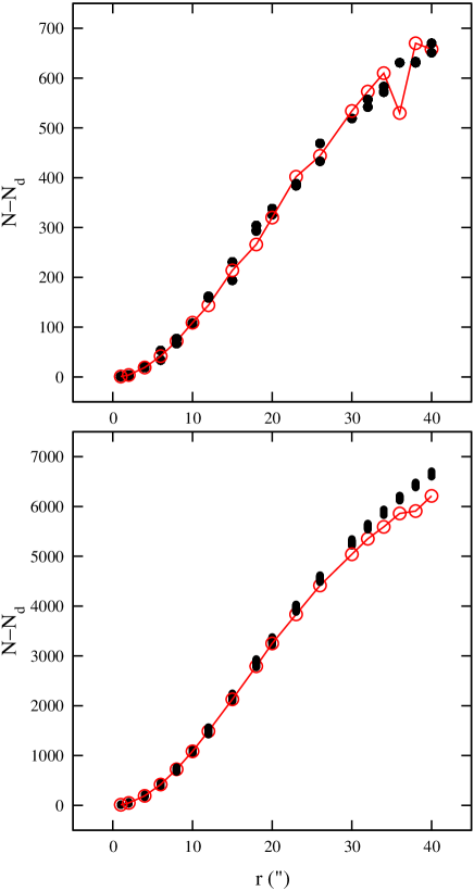
Figure 1: Blend losses as a function of confusion radius in 0.1 deg² (top) and 1 deg² (bottom) fields, where the stellar density was set to 10⁴ star/deg² in both fields. The heavily overlapping black dots represent one hundred simulations at each radius, while open circles connected with the solid lines show the predicted losses from Eq. 3.

2.3 The effects of double stars

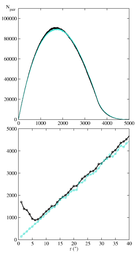
Figure 2: Pair-separation distributions for a 1 deg² field around V705 Cas (black line) and a random simulation (grey line). The lower panel is a zoom of the upper one showing the presence of about 5,000 resolved double stars.

We compare two histograms in Fig. 2. The thick black line shows the pair-distance distribution for USNO B1.0 stars around Nova (V705) Cas 1993 (21,520 stars with 14$\aas@@fstack{m}$00$<$red mag$<$17$\aas@@fstack{m}$99), while the grey line is for a simulation with 21,600 random points with the same field of view. As expected, the overall shapes of the distributions closely follow a Poisson-distribution, with slight boundary effect for the large distances (comparable to the diameter of the survey field), causing a somewhat sharper cut-off than a pure Poissonian.

We have three conclusions based on these kinds of comparisons for fields in the Milky Way:

• The overall distributions agree very well with the pure random simulations. There are slight indications for different shapes (see, e.g., the upper panel of Fig. 2 around $r=1500^{\prime\prime}$ and $3000^{\prime\prime}$), but the differences hardly exceed the intrinsic scatter of the data.

• The main disagreement occurs for the smallest pair-separations (typically for $r<10^{\prime\prime}$), which must be due to a large number of binary stars. For example, in the field around V705 Cas, the pair excess suggests about 5000 visual double stars with separations less than 7^′′. In denser regions even higher numbers can occur: the 1 deg² USNO B1.0 field around Nova (V4745) Sgr 2003 contains about 20,000 double stars with red mags$<$17$\aas@@fstack{m}$0 and separations under 10^′′. Considering that the Washington Double Star Catalogue (Mason et al. 2001) contains approximately 100,000 astrometric double and multiple stars, it is evident that most faint binary stars have yet to be identified and catalogued (see also Nicholson 2002).

• The contamination by physical binary stars can therefore be a significant factor that may distort the results of random blending.

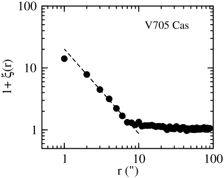
Figure 3: The two-point correlation function for the 1 deg² field around V705 Cas. The dashed line shows a power-law fit to the data between 2 and 8 arcsecs ($1+\xi(r)\sim r^{-1.3}$).

Star-star correlations can be taken into account with the two-point correlation function, $\xi(r)$, which is defined by the joint probability of finding an object in both of the surface elements $\delta S_{1}$ and $\delta S_{2}$ at separation $r_{12}$:

$$P=n^{2}~{}\delta S_{1}~{}\delta S_{2}[1+\xi(r_{12})].$$ (4)

Note that homogeneity and isotropy are assumed, so that $\xi$ is a function of the separation alone (Peebles 1980). If we can calculate this excess probability for pairs, then multiplying random blend losses from Eq. 3 by $(1+\xi(r_{c}))$ will correct the blending rate for the double stars. Neglecting higher correlation functions is a reasonable assumption, because the majority of stars belongs to single or double systems (about 90%, Abt 1983). Also, it is clear that even with this correction, the calculated blending rate will be a lower limit, because we do not have any information on the frequency of unresolved close binaries.

We can determine $\xi(r)$ using the recipe that leads to Eq. (47.14) in Peebles (1980): place $N_{t}$ points at random in the survey area; let $n_{p}(t)$ be the number of pairs among these trial points at separation $r$ to $r+\delta r$, and let $n_{p}$ be the corresponding number of pairs in the real catalogue of $N$ objects. Since $\xi=0$ for the trial points, the estimate of $\xi$ for the data is:

$$1+\xi(r)={n_{p}\over n_{p}(t)}{N_{t}^{2}\over N^{2}}.$$ (5)

We show an example in Fig. 3, which in our case is simply the ratio of the two histograms plotted in Fig. 2 (because $N_{t}$ was equal to $N$). The statistical uncertainty of the first point at $r=1^{\prime\prime}$ is $\pm 0.01$, far less than the symbol size, but a much larger systematic error is likely because that radius is comparable to the image scale of plates on which the catalogue is based. The dashed line in Fig. 3 shows a power-law fit ($\xi(r)\sim r^{\alpha}$) for the linear regime of the log-log plot. This diagram suggests that for the given dataset of 21,500 stars, the probability of finding two stars with 1 arcsec separation is about 20 times larger than for the pure random case. For a 1^′′ confusion radius Eq. 3 gives $N-N_{d}=56$, which means the corrected blending loss, including the measurable fraction of double stars, is about 1120 stars. In other words, the chance of being a blend in this dataset is at least 5.2%.

To conclude, it is always advisable to check star-star correlations before applying Eq. 3, and only if $\xi(r)$ is close to zero can we assume that double stars do not contribute significantly to blending (in practice, it means that the observations did not resolve binaries, probably because of the large distance).

3 Magnitude bias in the OGLE-II observations of the Large Magellanic Cloud

Our first application is an analysis of the OGLE-II $BVI$ observations of the Large Magellanic Cloud (Udalski et al. 2000). These data were obtained with the 1.3m Warsaw telescope at the Las Campanas Observatory for more than 7 million stars in the central 4.5 deg² of the LMC. The completeness of the resulting catalogue is high down to stars as faint as $B\approx 20$ mag, $V\approx 20$ mag and $I\approx 19.5$ mag. The median seeing of the observations was 1$\aas@@fstack{\prime\prime}$3, with no observations made when the seeing exceeded 1$\aas@@fstack{\prime\prime}$6–1$\aas@@fstack{\prime\prime}$8 (Udalski et al. 2000). Here we estimate blend losses in typical fields in the LMC and determine the corresponding magnitude biases in $V$ and $I$.

This is a Case 1 blending, since no existing catalogue has a smaller confusion radius than the OGLE-II observations, except small field-of-view observations with the Hubble Space Telescope (Olsen 1999), which were used to estimate MACHO blend biases by Alcock et al. (2001). To investigate possible photometric biases, we downloaded a representative field from the OGLE public archive. We chose LMC_SC5, centered at RA(2000)=$5^{\rm h}23^{\rm m}48^{\rm s}$, Dec(2000)=$-69^{\circ}41^{\prime}05^{\prime\prime}$, which contains about 460,000 stars. The majority of stars are fainter than 18 mag (both in $V$ and $I$), so we restricted the sample to stars between 18 mag and 21 mag. We used the two-point correlation function to constrain possible binarity effects and also to estimate the confusion radius. Because the stellar density varies gradually across the bar of the LMC, we selected several subsamples within which the density was constant. Here we discuss two of them, one in the middle of the bar (hereafter Region 1, $80.7<{\rm RA[^{\circ}]}<80.8$, $-69.7<{\rm Dec[^{\circ}]}<-69.6$) and one further south (hereafter Region 2, $80.7<{\rm RA[^{\circ}]}<80.8$ and $-70<{\rm Dec[^{\circ}]}<-69.9$). Other subsamples yield practically identical characteristics for blending systematics.

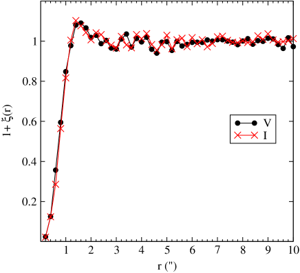
Figure 4: Two-point correlation functions in $V$ and $I$ in Region 1.

Table 2: Star counts, estimated total numbers of stars, blend losses and blending frequencies for two OGLE fields in the LMC.

Region	band	$N_{d}$	$N$	$N-N_{d}$	$(N-N_{d})/N_{d}$
1	$V$	7598	9151	1553	20%
2	$V$	5354	6081	727	14%
1	$I$	7728	9340	1612	21%
2	$I$	6073	7026	953	16%

In Fig. 4 we show the two-point correlation functions for Region 1 in $V$ and $I$ bands. The step size in radius was $\delta r=0\aas@@fstack{\prime\prime}2$, and we plotted the functions with linear scaling, so that changes around the confusion radius could be noticed more easily. We do not see a significant excess amount of correlated pairs, which is not surprising given the distance to the LMC. There is a slight rise of the correlation function for $1\aas@@fstack{\prime\prime}4\leq r\leq 3^{\prime\prime}$ that may be attributed to the widest binary stars. However, the correlation goes down quickly for $r<1\aas@@fstack{\prime\prime}0$. Since the best seeing of the OGLE images reached 0$\aas@@fstack{\prime\prime}$8 (Udalski et al. 1998), we adopt this value as the confusion radius. Our choice is also consistent with “critical radius” chosen as 0$\aas@@fstack{\prime\prime}$75 by the OGLE-team, within which objects were treated as identical (Udalski et al. 1998). The blend losses estimated using Eq. 3 are shown in Table 2.

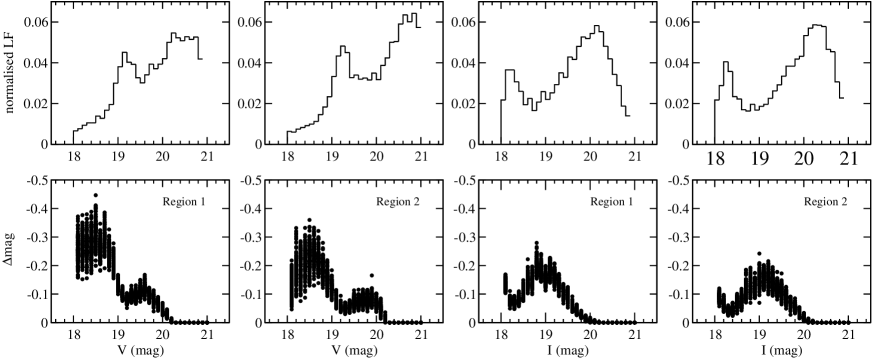
Figure 5: The luminosity functions in Region 1 and 2 (upper panels) and the calculated systematic magnitude biases (lower panels).

Apparently, about one in five-six stars is a blend having an unresolved companion that is within 3 mags in brightness (since our data sample covers the range 18 to 21 mag). We have to stress that these numbers are only lower limits because of the incompleteness of the OGLE data below $\sim$20 mag, which means the systematic errors we derive are still underestimated. Our main purpose is to point out the existence of surprisingly large systematic errors that can be determined from a single dataset alone. Deeper data (like in Alcock et al. 2001) would only shift these systematics toward larger values, but that is beyond the scope of the present paper.

Having estimated the fraction of blended stars, we are now in a position to calculate the extent to which they will bias the photometry. We assume that the probability of a star blending with a neighbour does not depend on its brightness, so that blended and unblended stars have the same luminosity function (LF) within each region. This is likely to introduce a slight systematic error, but we estimate this to have a marginal effect on the final outcome of the investigation. Upper panels in Fig. 5 contain the normalized $V$ and $I$ luminosity functions ($\sum_{18}^{21}{\rm LF}(m)=1$), where the prominent peaks at $V\approx 19$ mag and $I\approx 18$ mag correspond to the red clump (Udalski 2000). The $I$-band decline for $I>20$ mag shows the decreasing completeness (see Table 4 in Udalski et al. 2000), which is less severe in $V$. The next step was to carry out a Monte Carlo simulation for each region and each filter: we placed $N$ stars at random into the given survey area, where $N$ is the corresponding number in the fourth column of Table 2. The luminosity function was set to the one shown in Fig. 5. Then we determined which stars were “blends” in the random set and calculated the integrated magnitude of each blend. The magnitude difference between the blend and the brightest star within it was assigned as a bias at the integrated magnitude. Finally, these bias values were averaged for every 0.1 mag bin of the luminosity function (unblended stars were taken into account by adding zero bias). The whole procedure was repeated one hundred times and the results are shown in the lower panels of Fig. 5. Small changes to the input luminosity functions affected the final bias distributions at a level lower than the scatter visible in the plots.

We can draw several conclusions based on Fig. 5. Firstly and most importantly, blending introduces systematic errors as large as 0$\aas@@fstack{m}$2–0$\aas@@fstack{m}$3 (for instance, the mean bias between $V=18-19$ mag is 0$\aas@@fstack{m}$25 in Region 1 and 0$\aas@@fstack{m}$18 in Region 2), which can have serious consequences if neglected. Details of OGLE-II reduction, tests of photometric accuracy and incompleteness were published in Udalski et al. (1998) and they did not mention random blending as a possible source of systematic biases. Very recently, Alcock et al. (2004) presented an analysis of first-overtone RR Lyrae stars in the MACHO database, for which systematic magnitude biases due to blending were also estimated. At $V\approx 19\aas@@fstack{m}3$, where RR Lyrae stars concentrate, Alcock et al. (2004) arrived at $\Delta V$ ranging from $-0\aas@@fstack{m}11$ to $-0\aas@@fstack{m}21$ for various assumptions (they made artificial star tests for various stellar densities and calculated the differences between the input and recovered magnitudes of artificial stars). Our results are based on a very different approach applied to a very different dataset, and the agreement suggests that random blending must be taken into account in such high-level crowding as the present one. Secondly, the gradual decrease of the bias towards fainter magnitudes shows the effect of incompleteness: as was shown by Alcock et al. (2001) for the MACHO database, systematic errors increase monotonically over the examined magnitude range. For that reason, the calculated biases between 18 and 19 mag can be considered as lower limits for the fainter magnitudes; the magnitude range of RR Lyrae stars is therefore very likely to suffer from a bias up to 0$\aas@@fstack{m}$2–0$\aas@@fstack{m}$3, which has been neglected in the past. This leads to our third conclusion: results based on the OGLE-II data that supported the LMC “short” distance scale ($(m-M)_{\rm LMC}\approx 18\aas@@fstack{m}3$) are likely to suffer from this systematic error. For example, Udalski (2000) calibrated the zero-point of the distance scale using RR Lyrae variables and red clump stars to be $(m-M)_{\rm LMC}=18\aas@@fstack{m}24$ with 0$\aas@@fstack{m}$07 systematic error. However, blending correction significantly decreases the apparent conflict between this and the “standard” value (18$\aas@@fstack{m}$5, e.g. Alves 2004), which shows the importance of blending biases.

It must be stressed that ground-based observations of more distant galaxies may suffer from even larger systematic errors. Detecting variable stars by the image subtraction method circumvents the problem (see a recent application by Bonanos & Stanek 2003), but measuring apparent magnitudes (and hence distance) requires use of space telescopes. Calculations like the present one can help estimate systematics but more reliable results for nearby galaxies need high-resolution observations.

4 Field star distributions around seven recent novae

Table 3: Seven bright nova outbursts with reported progenitor candidates in the last decade.

Star (year)	Progenitor details	Ref.
V1494 Aql (1999/2)	Red mag 15$\aas@@fstack{m}$6	1
V2275 Cyg (2001)	Red mag 18$\aas@@fstack{m}$8 (USNO A2.0)	2
V382 Vel (1999)	Quiescent magnitude $V=16\aas@@fstack{m}56$	3
V4743 Sgr (2002/2)	Red mag 16$\aas@@fstack{m}$7 (USNO A2.0)	4
V4745 Sgr (2003)	DSS red plate, $R\approx 17\aas@@fstack{m}9$, apparently
	blended with a faint companion to SE	5
V705 Cas (1993)	Candidate precursor of red mag about
	17$\aas@@fstack{m}$0, northern component of a merged
	pair with separation about 2 arcsec	6, 7
V723 Cas (1995)	DSS red plate, mag 18-19	8

References: 1 – Pereira et al. (1999); 2 – Schmeer (2001); 3 – Platais et al. (2000); 4 – Haseda et al. (2002); 5 – Brown et al. (2003); 6 – Skiff et al. (1993); 7 – Munari et al. (1994); 8 – Hirosawa et al. (1995)

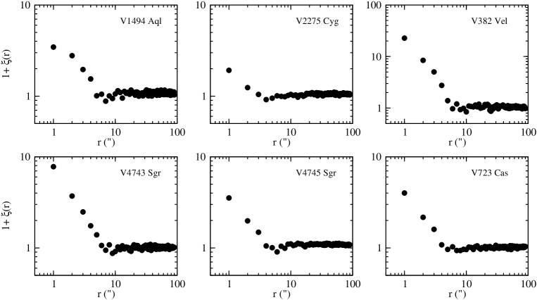
Figure 6: Two-point correlation functions around six novae.

Table 4: Statistical properties of the examined datasets. Abbreviations: $N_{d}$ – number of stars within the specified magnitude range; $N(m<m_{u})$ – total number of stars brighter than the fainter limit; $\Delta N$ – random blend loss via Eq. 3; $\xi(r_{c})$ – the two-point correlation function at $r_{c}=1\aas@@fstack{\prime\prime}5$; blend rate – blending occurrence rate, corrected by $1+\xi(r)$; A1 – the probability that the pre-outburst star coincides with the nova by chance; A2 – the probability that the optical companion is correlated with the nova itself.

Star	Mag range	$N_{d}$	$N(m<m_{u})$	$\Delta N$	$1+\xi(r_{c})$	blend	A1	A2
						rate
V1494 Aql	15–16	8,333	13,229	19	4	0.9%	0.5%	75%
V2275 Cyg	18–19	22,249	47,255	137	1.5	0.9%	1.2%	–
V382 Vel	16–16.6	6,125	19,291	10	15	2.4%	0.3%	–
V4743 Sgr	16–17	10,775	20,165	32	5	1.5%	0.6%	–
V4745 Sgr	17–18.5	35,997	62,042	485	3	4%	2.7%	–
V705 Cas	16.5–17.5	8,066	17,374	18	10	2.2%	0.5%	90%
V723 Cas	18–19.5	18,932	31,302	99	3	1.6%	1%	–

Our next case study was inspired by the independent discovery of the close optical companion of nova V1494 Aql (Kiss et al. 2004). We selected several bright nova outbursts in the last decade for which progenitor star candidates have been identified in Digitized Sky Survey plates or deep star catalogues (most often in the USNO A1.0 and A2.0 catalogue releases). The available details on these candidates are summarized in Table 3. We examined the following questions: How probable is it that the candidates are unrelated stars located only by chance at the nova coordinates? In cases where a star was found a few arcseconds from the nova position, (like for V1494 Aql and V705 Cas), how probable is is that they are physically related to the nova system?

To find out the answers, we downloaded and analysed 1 deg² USNO B1.0 fields around each nova using the USNO Flagstaff Station Integrated Image and Catalogue Archive Service . These fields provide a complete coverage down to $V=21\aas@@fstack{m}0$, 0$\aas@@fstack{\prime\prime}$2 astrometric accuracy at J2000, 0.3 mag photometric accuracy in up to five colours and 85% accuracy for distinguishing stars from nonstellar objects (see Monet et al. 2003 for more details). The latter issue is less relevant in these fields because of the low galactic latitudes. In two cases we found incompleteness of the data, either in the form of large empty areas in the given field (V4745 Sgr) or sudden jumps in the stellar density within certain rectangular areas (V4743 Sgr). Both fields are located in the densest regions of the Milky Way, which explains the difficulties of measuring wide-field Schmidt-plates in such crowded fields. We took these into account in our analysis (e.g. in the latter case we omitted patches of lower density, yielding a decreased survey area).

Since this is Case 1 blending, we calculated random blend losses for each nova by choosing all stars within 1–1.5 mag in brightness of the reported progenitor (when the accuracy was worse, we chose the wider range). For this, we used red magnitude data in the catalogue. We assumed a 1$\aas@@fstack{\prime\prime}$5 confusion radius, based on the pixel scale of the scanned Schmidt-plates (usually about 0$\aas@@fstack{\prime\prime}$9/pixel, Monet et al. 2003) and the fact that the optical companion of V1494 Aql located at 1$\aas@@fstack{\prime\prime}$4 was unresolved in the data. Two-point correlation functions (Fig. 6) were determined via Eq. 5, filling up the survey areas by 25,000 points at random. Blend losses were then multiplied by the two-point correlation functions at $r=1\aas@@fstack{\prime\prime}5$. Finally, we calculated the chance of finding a random blend within 1$\aas@@fstack{\prime\prime}$5 of the nova coordinates. We summarize the results in Table 4 and in Fig. 6 (for V705 Cas we got essentially the same as in Fig. 3 for a wider magnitude range, so that there was no reason to repeat the plot).

It is evident from Fig. 6 that the samples are dominated by binary stars in every field for separations under $\sim 10^{\prime\prime}$. The highest correlation was found around V382 Vel, where the number of 1-arcsec doubles exceeds the number expected for a random field by a factor of 23! In other words, at least 22 of every 23 1-arcsec pairs are physically related (binary) stars. It is also prominent that there is a slope decrease in every correlation function for the smallest radii, which we interpret as a result of confusion losses. For that reason, we estimated $\xi(r_{c}=1\aas@@fstack{\prime\prime}5)$ (6th column in Table 4) from extrapolated linear fits over the log-log plot of the 2–6 arcsecs data, rather than from interpolations between 1 and 2 arcsecs.

The numbers in Table 4 clearly show that random blend loss stays well below 1%; even for the worst case, V4745 Sgr, it is only 1.4% of $N_{d}$. After multiplying by the estimated two-point correlation function values, the blending rate still remains around 1–2%. The eighth column in Table 4 (A1) confirms that progenitors can be identified with high confidence, even in the central regions of the Milky Way.

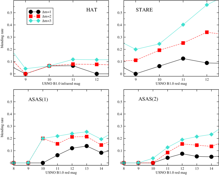
Figure 7: Blending rates for similar projects at four different galactic latitudes (HAT: $+30^{\circ}$; STARE: $+2^{\circ}$; ASAS(1): $-60^{\circ}$; ASAS(2): $-20^{\circ}$). The confusion radius is about $20^{\prime\prime}$ for each project.

The most interesting numbers can be found in the last column of Table 4. They follow from the probability interpretation of the two-point correlation function. Since $(1+\xi(r))$ reflects the excess probability for finding a pair in a sample at distance $r$, $1+\xi(r)=4$ (first row in Table 4) means that there are four times more pairs than in a random sample, so that for any given pair the chance of being correlated is 75%. Therefore, these data suggest that it is quite possible that the optical companions of V1494 Aql and V705 Cas form wide hierarchical triple systems with the cataclysmic components. Interestingly, for V1494 Aql this is also supported by our knowledge of the optical companion. In Kiss et al. (2004) we assigned late F-early G as an approximate spectral type of the companion. The corresponding absolute magnitude for a main sequence star is about $M_{V}=$+4$\aas@@fstack{m}$0, which agrees within the error bars with the quiescent absolute magnitude of the nova (Kiss et al. 2004). Hence, the close apparent magnitudes of the pre-nova and the companion suggest similar distances, consequently the possibility of physical correlation. For V705 Cas, we do not have similar supporting evidence, but it is an intriguing possibility that these optical components are in triple systems with the novae. If confirmed, their presence could be used, for example, to derive independent distances via spectroscopic parallaxes, which in turn would allow one to calculate accurate absolute magnitudes of the nova eruptions.

This case study shows that seeing-limited images are not significantly affected by random blending, even in the galactic plane. We now turn to the case of images with much lower spatial resolution.

5 Wide-field photometric surveys

In the recent years there has been an explosion in the number of small and medium-sized robotic telescopes that monitor selected regions of the sky with various instruments (e.g., Hessman (2004) listed 80 different projects). We selected three representative small instruments that are currently running, to investigate Case 2 blending. They are:

1. The Hungarian Automated Telescope (HAT) which, in its present status, observes stars between $I=9-12$ mag in selected fields of the northern sky. The data were reduced with PSF-fitting photometry (Bakos et al. 2004). We downloaded the 1 deg² USNO B1.0 field in Hercules (RA(2000)=$17^{\rm h}36^{\rm m}$, Dec(2000)=$37^{\circ}30^{\prime}$, $b\approx 30^{\circ}$).

2. The STellar Astrophysics & Research on Exoplanets (STARE) project, observing between $R=9-12\aas@@fstack{m}5$ in various fields (Alonso et al. 2003, Brown 2003). We downloaded the 1 deg² USNO B1.0 field, centered at RA(2000)=$20^{\rm h}06^{\rm m}$, Dec(2000)=$36^{\circ}00^{\prime}$ ($b\approx 2^{\circ}$).

3. The All Sky Automated Survey (ASAS), which covers over 1 million stars in the southern hemisphere between $V=8\aas@@fstack{m}5-15$ mag. The data are reduced with simple aperture photometry (Pojmanski 2002, 2004). We selected two 1-deg² fields at random at two different galactic latitudes: RA(2000)=$00^{\rm h}19^{\rm m}$, Dec(2000)=$-56^{\circ}00^{\prime}$ ($b\approx-60^{\circ}$) and RA(2000)=$06^{\rm h}10^{\rm m}$, Dec(2000)=$-23^{\circ}00^{\prime}$ ($b\approx-20^{\circ}$).

Each project is characterized by $r_{c}\approx 20^{\prime\prime}$, so that their comparison reveals the differences that depend on the galactic latitude. To match the photometric bands used in these projects, we examined USNO B1.0 infrared magnitudes for the HAT-field and red magnitudes for the remaining regions. The main aim was to get an idea of the fraction of biased stars, because although crowding problems are well-known for these instrumental setups, we did not find any quantitative description of the issue. Therefore, we calculated blending rates for various $m$ and $\Delta m$ values that covered the magnitude ranges of the projects. This rate was defined as the following ratio:

$${\rm blending~{}rate}={\nu(m,\Delta m,r_{c})\over\nu(m)},$$ (6)

where $\nu(m,\Delta m,r_{c})$ is the number of stars which have fainter neighbours within a distance $r_{c}$ and magnitude difference $\Delta m$; $\nu(m)$ is the total number of $m$ magnitude stars (in our case, defined as stars with apparent brightnesses within $m$ and $m+1$ mag). We assumed negligible blend losses in the USNO B1.0 catalogue over the studied magnitude and separation ranges. The results are shown in Fig. 7. We also determined two-point correlation functions, which showed that for these bright magnitudes the overwhelming majority of pairs closer than the confusion radius are physically related double stars.

Figure 7 implies an alarming rate of blending, even for high galactic latitudes. We see that 10 to 20 percent of objects observed by the HAT and ASAS projects have blends within 3 mags, while up to 50% are affected near the galactic plane (STARE). Correlated pairs can make the situation quite bad even for the brightest stars, which means blending must be taken into account in every case. Presently available star catalogues offer a good opportunity to do that, thus we recommend to add blending information in all cases when finally reduced data are made accessible to the wider community. Also, the implementation of the image subtraction method (Alard & Lupton 1998) is highly desirable in this type of project, because the photocenter of the variable source can be used to identify which object within a blend is varying (Alard 1996; see also Hartman et al. 2004).

6 Conclusions

In this study we investigated the effects of random blending that involves stars of similar brightnesses, leading to significant biases in the measured apparent magnitudes and amplitudes. A simple formula (Eq. 3) was derived to calculate blend losses in a real catalogue of stars based on the confusion radius, total number of detected stars and survey area. We showed that the two-point correlations must be included in calculations when studying galactic fields, where binary stars dominate for separations under 10^′′. Outside the Milky Way, we quickly lose the information on wide binaries, so that the pure random case applies. That is why the calculated blending rate always puts only a lower limit to the full blending.

We discussed three different applications, which demonstrate the importance of these phenomena. The most interesting results were presented for the OGLE-II data of the Large Magellanic Cloud. With extremely high stellar angular densities, these observations are much more biased by random blending than those fields in the galactic plane. Even though no observations were carried out for seeing larger than 1$\aas@@fstack{\prime\prime}$6–1$\aas@@fstack{\prime\prime}$8, we estimated that 15-20% of the sample are affected by blends that are within three magnitudes in apparent brightness. The resulting magnitude biases can reach 0$\aas@@fstack{m}$2–0$\aas@@fstack{m}$3, depending on the angular position within the LMC. This allows us to reconcile the OGLE-based distance moduli of the LMC ($\mu\approx 18\aas@@fstack{m}3$) and the generally adopted “standard” one ($\mu\approx 18\aas@@fstack{m}5$). Random blend calculations are therefore highly desirable in every case when significant blending is expected, especially in extragalactic observations.

The analysis of star fields around seven novae showed that progenitor identification is very secure, even in the extremely dense fields of the Bulge. Furthermore, statistical evidence points toward the existence of wide hierarchical triple systems, in which the third component lies at 1–2^′′ (i.e. several thousand AU) from the novae. Thus, it is highly desirable to measure proper motions for V1494 Aql and V705 Cas and their optical companions to confirm or reject the physical correlations.

In our last example we demonstrated high-blending rates in typical wide-field photometric surveys for exoplanet transits. In certain cases, up to 50–60% of stars can be affected by blending objects within 3 magnitudes. We recommend that cross-correlation with appropriate star catalogues should always be done as part of the regular data reduction, to flag every possibly problematic star.

Our presented method for calculating blend losses is very simple, thus may not be applicable in certain cases. For instance, when the stellar angular density shows strong gradient, like in a globular cluster or outer parts of a resolved galaxy, the basic assumption of homogeneity and isotropy will be invalid. A possible solution in such cases is to introduce a position-dependent density $n=\rho(x,y)$, where $x$ and $y$ are the image coordinates, and to integrate all equations over the inhomogeneous and anisotropic sample. In principle, the numeric implementation of this generalisation is not too difficult. Another way to treat these cases is to split the data into small segments within which $n\approx{\rm const.}$ and, after calculating blending biases, take averages over the segments.

To summarize, the experience with real datasets suggests that it is always highly advisable to estimate random blend losses when the star density and/or the confusion radius have relatively large values – Eq. 3 or deep star catalogues can be used to characterize any specific example. Where applicable, the upgrade from aperture and PSF-photometry to the image subtraction method is desirable to reduce some of the blending effects.

References

- [] Abt H.A., 1983, ARA&A, 21, 343
- [] Alard C., 1996, IAU Symp. 173, 215
- [] Alard C., 1997, A&A, 321, 424
- [] Alard C., & Lupton R.H., 1998, ApJ, 503, 325
- [] Alcock C., et al., 2001, ApJS, 136, 439
- [] Alcock C., et al., 2004, AJ, 127, 334
- [] Alonso R., Belmonte J.A., & Brown T., 2003, ApSS, 284, 13
- [] Alves D.R., 2004, in: Highlights of Astronomy, Vol. 13, in press, (astro-ph/0310673)
- [] Antonello E., 2002, A&A, 391, 795
- [] Bakos G.Á, Lázár J., Papp I., Sári P., & Green E.M., 2002, PASP, 114, 974
- [] Bakos G., Noyes R.W., Kovács G., Stanek K.Z., Sasselov D.D., & Domsa I., 2004, PASP, 116, 266
- [] Bonanos A.Z., & Stanek K.Z., 2003, ApJ, 591, L111
- [] Brown T.M., 2003, ApJ, 593, L125
- [] Brown J., et al., 2003, IAUC, No. 8123, 1.
- [] Ferrarese L., Silbermann N.A., Mould J.R., Stetson P.B., Saha A., Freedman W.L., & Kennicutt Jr. R.C., 2000, PASP, 112, 177
- [] Gibson B.K., Maloney P.R., & Sakai S., 2000, ApJ, 530, L5
- [] Han C., 1997, ApJ, 490, 51
- [] Han C., 1998, ApJ, 500, 569
- [] Harris J., & Zaritsky D., 1999, AJ, 117, 2831
- [] Hartman J.D., Bakos G., Stanek K.Z., & Noyes R.W., 2004, AJ, submitted (astro-ph/0405597)
- [] Haseda K., et al., 2002, IAUC, No. 7975, 1.
-
[]
Hessman F.V., 2004, http://www.uni-sw.gwdg.de/hessman/
MONET/links.html - [] Hirosawa K., Yamamoto M., Nakano S., Kojima T., Iida M., Sugie A., Takahashi S., & Williams G.V., 1995, IAUC, No. 6213, 1.
- [] Kiss L.L., Csák B., & Derekas A., 2004, A&A, 416, 319
- [] Mason B.D., Wycoff G.L., Hartkopf W.I., Douglass G.G., & Worley C.E., 2001, AJ, 122, 3466
- [] Mochejska B.J., Macri L.M., Sasselov D.D., & Stanek K.Z., 2000, AJ, 120, 810
- [] Monet D.G., et al., 2003, AJ, 125, 984
- [] Munari U., Tomov T., Hric L., & Hazucha P., 1994, IBVS, No. 3977
-
[]
Nicholson M.P., 2002, http://ad.usno.navy.mil/wds/
unpublished/nicholson.html - [] Olsen K.A.G., 1999, AJ, 117, 2244
- [] Peebles P.J.E., 1980, The Large-Scale Structure of the Universe (Chapter III), Princeton University Press, Princeton
- [] Pereira A., di Cicco D., Vitorino C., & Green D.W.E., 1999, IAUC, No. 7323, 1.
- [] Platais I., Girard T.M., Kozhurina-Platais V., van Altena W.F., Jain R.K., & López C.E., 2000, PASP, 112, 224
- [] Pojmanski G., 2002, Acta Astron., 52, 397
- [] Pojmanski G., 2004, Acta Astron., in press (astro-ph/0401125)
- [] Schmeer P., 2001, IAUC, No. 7688, 2.
- [] Skiff B., Abe H., & Bengtsson H., 1993, IAUC, No. 5904, 2.
- [] Snel R.C., 1998, A&AS, 129, 195
- [] Takeuchi T.T., & Ishii T.T., 2004, ApJ, 604, 40
- [] Udalski A., 2000, Acta Astron., 50, 279
- [] Udalski A., Szymanski M., Kubiak M., Pietrzynski G., Wozniak P., & Zebrun K., 1998, Acta Astron., 48, 147
- [] Udalski A., et al., 2000, Acta Astron., 50, 307
- [] Wozniak P., & Paczynski B., 1997, ApJ, 487, 55