Supernova Rates in Galaxy Clusters

Abstract

Measurements of SN rates in different environments and redshifts can shed light on the nature of SN-Ia progenitors, star formation history, and chemical enrichment history. I summarize some recent work by our group in this area, and discuss the implications. The current evidence favors production of most of the iron in the ICM (and perhaps everywhere) by core-collapse SNe, rather than SNe-Ia. These SNe may have been produced by the first, top-heavy-IMF, generation of stars that reionized the Universe. Improved rate measurements can sharpen the picture, and I describe our recent efforts in this direction.

School of Physics and Astronomy, Tel-Aviv University, Tel-Aviv 69978, Israel; maoz@wise.tau.ac.il

Learning what are the progenitors of the different types of SNe, what are their rates, and what are their distributions in space and in cosmic time, are essential steps toward understanding SN physics, cosmic metal enrichment, and galaxy formation (e.g., Kobayashi et al. 2000). Core-collapse SNe explode promptly ($\mathrel{\hbox{\hbox to0.0pt{\hbox{\lower 4.0pt\hbox{$\sim$}}\hss}\hbox{$<$}}}10$ Myr) after the formation of a stellar population, and their rate traces the star-formation history (SFH). In contrast, SN-Ia explosions should occur only after WD formation and binary evolution, with a “delay” of order 0.1–10 Gyr. The SN-Ia rate vs. cosmic time will therefore be a convolution of the SFH with a “delay function,” the SN-Ia rate following a brief burst of star formation. Each of the SN-Ia progenitor scenarios predicts a different delay function (e.g., Madau et al. 1998; Yungelson & Livio 2000), which in turn dictates the SN rate vs. redshift.

SN rate measurements in rich galaxy clusters at redshifts $0<z<1$ are particularly relevant for constraining the SFH in different environments, the progenitors of the different SN types, and the contribution of each type to cosmic metal enrichment. Clusters are useful places to study enrichment because their deep potentials make them “closed boxes” from which little matter can escape. The intra-cluster medium (ICM), which contains about 90% of the baryons in clusters, has a high metallicity. The iron abundance, in particular, is the one most easily and robustly measured, because iron has the strongest X-ray emission line in clusters, and because the theoretical conversion from data to abundance is simple (the line is dominated by emission from He-like ions). It is widely agreed that massive clusters have a “canonical” iron abundance of $0.3Z_{\odot}$, with little dependence on cluster mass (e.g., Lin et al. 2003) or redshift, out to $z\approx 1$ (Tozzi et al. 2003; Hashimoto et al. 2004). Furthermore, the iron production of the various SN types is observationally well constrained — the radioactive decay of nickel to cobalt to iron drives much of the optical luminosity of SNe, and thus empirical SN light curves yield direct estimates of the ejected iron mass. It is easy to show that, including also the mass of iron locked in the stellar component of a cluster, the total iron mass in clusters is surprisingly large (e.g., Renzini et al. 1993; Maoz & Gal-Yam 2004). If core-collapse SNe were the prime source of the iron in clusters, there is a factor of $\sim 5$ excess of observed iron mass, compared with expectations, given the observed present-day stellar mass.

Figure 1.: Cluster SN-Ia rates vs. redshift — predictions and observations. Left panel is a zoom-in on the low-redshift portion of the right panel. Rate curves follow the prescription of Madau et al. (1998), for stellar formation redshift $z_{f}=2$ and SN-Ia delay times of 0.5, 1, 2, or 3 Gyr. The curves are normalized to produce the observed iron-mass-to-light ratio of rich clusters (Maoz & Gal-Yam 2004). Filled circles are the measurements of Gal-Yam et al. (2002) based on HST/WFPC2 data. Empty circles illustrate the mean redshifts of our three ongoing measurements at different redshifts, plotted at arbitrary levels.

A proposed solution to this puzzle is that clusters were enriched by a stellar population with a “top-heavy” IMF, i.e., with relatively many high-mass stars, exploding as iron-producing, core-collapse SNe — perhaps the deaths of the first, very massive stars, that reionized the Universe at $z\approx 10$ (e.g., Loewenstein 2001). Most of the cluster stars seen today would then have formed from the pre-enriched gas. Alternatively, most of the cluster iron may have been produced by SNe-Ia from the normal stellar population. In principle, one could discriminate between the two solutions using the observed elemental mix in the ICM, relative to iron, compared to theoretical SN model yields. However, no consensus has emerged, due to the observational and theoretical uncertainties in the analysis of non-iron elements (e.g., Buote 2002 vs. Lima-Neto et al. 2003).

Measurement of SN rates vs. redshift (i.e., look-back time) offers a different, direct route of investigating the source of the iron. The SN-Ia enrichment scenario requires a large total number of SNe-Ia, integrated over the cluster lifetime. Since present SN-Ia rates are low, the SN-Ia rate must have been much higher in the past. Indeed, for an assumed star-formation epoch in clusters ($z_{f}\approx 2$, based on the fundamental plane; van Dokkum & Franx 2001) and a given SN-Ia delay function, one can predict the cluster SN-Ia rate, SNR${}_{Ia}(z)$, required to produce the observed iron mass. Figure 1 shows an example of such a set of predictions. Measurement of SNR${}_{Ia}(z)$ can not only reveal the iron source directly (if it is SNe-Ia), but can also place observational constraints on the SN-Ia delay function, and hence on the progenitor scenario.

Gal-Yam, Maoz, & Sharon (2002) carried out a first measurement of cluster SN-Ia rates at high $z$ using HST archival data for eight rich clusters. In Maoz & Gal-Yam (2004), the measured rates at $z=0.25$ and $z=0.9$ were compared to those predicted by the SN-Ia iron production scenario. As seen in Fig. 1, the upper limit on the SNR at $z\approx 1$ argues against models with long SN-Ia time delays, predicting SN rates ten times higher than observed. Thus, cluster iron production by SNe-Ia appears to be a viable option only if SNe-Ia have short ($\mathrel{\hbox{\hbox to0.0pt{\hbox{\lower 4.0pt\hbox{$\sim$}}\hss}\hbox{$<$}}}2$ Gyr) time delays. Interestingly, comparison of the SNR${}_{Ia}(z)$ in the field to the cosmic star formation history suggests a long delay time (Pain et al. 2002; Tonry et al. 2003; Gal-Yam & Maoz 2004; Strolger et al. 2004; Dahlen et al. 2004). The results therefore point to core-collapse SNe from an early, top-heavy IMF, stellar generation as the source of cluster enrichment. Alternatively, the existence of two distinct SN-Ia progenitor populations – an “old” one in clusters and a “young” one in the field – is also an option (Mannucci et al. 2004). However, small-number statistics are the major limiting factor in current estimates of SNR${}_{Ia}(z)$, and in constraints on SN-Ia delay functions.

To remedy this situation, we are engaged in obtaining accurate measurements of the SN-Ia rate in several samples of rich clusters. Three different observing programs, currently at various stages of execution, will measure the rate in three different redshift ranges, as follows.
The Wise cluster SN survey; $0.08<z<0.2$ – In 1998–2001 we carried out a SN survey, using the Wise 1-m telescope, on a sample of rich clusters at $0.08<z<0.2$. Among the results of this survey were the first two clear examples of intergalactic cluster SNe-Ia (Gal-Yam et al. 2002). Spectroscopic followup of all candidates or their hosts has been completed at large telescopes, mainly Keck. We therefore now have a “clean” sample of seven transients, each spectroscopically confirmed as a cluster SN-Ia (see Fig. 2), with

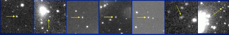
Figure 2.: Seven cluster SNe-Ia discovered at Wise and spectroscopically confirmed at Keck and other telescopes. From left to right, SNe 1998eu, 1998fc, 1999cg, 1999ch, 1999ci, 1999ct, 2001al. These SNe will be used to calculate the cluster SN-Ia rate at $0.08<z<0.2$.

all other candidates from the survey having been demonstrated to not have been cluster SNe-Ia. To derive the SN-Ia cluster rate in this redshift interval, we are determining the detection efficiency. This will allow computation of the control time for the survey, and hence the SN rate (e.g., Gal-Yam et al. 2002).
The NOT cluster SN survey; $0.2<z<0.3$ – In the summer of 2004 we completed the imaging part of a cluster SN survey in this redshift range, using the 2.6-m Nordic Optical Telescope (NOT) in La Palma. A number of candidates have been confirmed as cluster SNe-Ia using Keck spectroscopy (see Fig. 3 for an example),

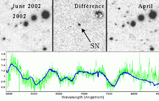
Figure 3.: Discovery images from the NOT of SN 2002lh, and a Keck spectrum showing it is a SN-Ia at the redshift of Abell 1961 ($z=0.236$). Solid curve is a spectrum of nearby SN-Ia 1999ee, suitably redshifted. This and other cluster SNe will be used to derive a cluster SN-Ia rate at $0.2<z<0.3$.

and we continue the followup work on the less-promising transients — these generally have turned out to be active galactic nuclei (AGNs), variable stars, and SNe in the background or foreground of a cluster. We will determine the detection efficiencies for this survey as well, and derive the cluster SN-Ia rate in this redshift interval.
The Keck cluster SN survey; $0.3<z<0.5$ – We have been granted Keck observing time (PI A. Gal-Yam) to measure the SN-Ia rate in a complete sample of X-ray-selected $0.3<z<0.5$ clusters. The first run, in October 2004, successfully obtained $B$ and $R$ reference images for part of the sample. Subsequent runs will yield SNe. As in the nearer samples, followup work and efficiency simulations will result in a SN-Ia rate determination for this redshift bin.

References

- (1) Buote 2002, ApJL, 574, L135
- (2) Dahlen et al. 2004, ApJ, 613, 189
- (3) Gal-Yam, Maoz, & Sharon 2002, MNRAS, 347, 942
- (4) Gal-Yam, Maoz, Guhathakurta, & Filippenko 2003, AJ, 125, 1087
- (5) Gal-Yam & Maoz 2004, MNRAS, 347, 942
- (6) Hashimoto et al. 2004, astro-ph/0401297
- (7) Kobayashi et al. 1998, ApJ, 503, L155
- (8) Lima Neto, Capelato, Sodré, & Proust 2003, A&A, 398, 31
- (9) Lin, Mohr, & Stanford, 2003, ApJ, 591, 749
- (10) Loewenstein 2001, ApJ, 557, 573
- (11) Madau et al. 1998, MNRAS, 297, L17
- (12) Maoz & Gal-Yam 2004, MNRAS, 347, 951
- (13) Mannucci, et al. 2004, A&A, in press, astro-ph/0411450
- (14) Pain et al. 2002, ApJ, 577, 120
- (15) Renzini et al. 1993, ApJ, 419, 52
- (16) Strolger et al. 2004, ApJ, 613, 200.
- (17) Tonry et al. 2003,ApJ, 594, 1
- (18) Tozzi et al. 2003, ApJ, 593, 705
- (19) van Dokkum & Franx, 2001, ApJ, 553, 90
- (20) Yungelson & Livio 2000, ApJ, 528, 108