An overdensity of galaxies at $z=5.9\pm 0.2$ in the Ultra Deep Field confirmed using the ACS grism

Abstract

We present grism spectra taken with the Advanced Camera for Surveys to identify 29 red sources with ($i_{775}$-$z_{850}$) $\geq 0.9$ in the Hubble Ultra Deep Field (HUDF). Of these 23 are found to be galaxies at redshifts between z=5.4 and 6.7, identified by the break at 1216 Å due to IGM absorption; two are late type dwarf stars with red colors; and four are galaxies with colors and spectral shape similar to dust reddened or old galaxies at redshifts z $\approx 1-2$. This constitutes the largest uniform, flux-limited sample of spectroscopically confirmed galaxies at such faint fluxes ($z_{850}$$\leq$ 27.5). Many are also among the most distant spectroscopically confirmed galaxies (at redshifts up to z=6.7).

We find a significant overdensity of galaxies at redshifts $z=5.9\pm 0.2$. Nearly two thirds of the galaxies in our sample (15/23) belong to this peak. Taking into account the selection function and the redshift sensitivity of the survey, we get a conservative overdensity of at least a factor of two along the line-of-sight. The galaxies found in this redshift peak are also localized in the plane of the sky in a non-random manner, occupying about half of the ACS chip. Thus the volume overdensity is a factor of four. The star-formation rate derived from detected sources in this overdense region is sufficient to reionize the local IGM.

1 Introduction

While theory (e.g. Press & Schechter 1974) and numerical simulations can tell us about the gravitational collapse and clustering of dark matter, the onset of star-formation in galaxies is complicated enough that observations are required to guide the theory. The question about how biased the early star-formation is can be addressed by measuring clustering at the highest redshifts accesible.

The Hubble Ultra Deep Field provides a uniquely deep look at the universe in its infancy. With visible and near-infrared observations reaching a depth of $z_{850}$$=28.2$ and $J=26.85$ AB magnitudes (10$\sigma$ for $0."5$ aperture) (Beckwith et al. 2004 in prep., Thompson et al. 2005, Bouwens et al. 2004), one can reliably detect galaxies as faint as $0.02\times L_{*}$ at $z\approx 6$ (Yan & Windhorst 2004, Bunker et al. 2004). Because of its depth this is potentially a good field to study formation and clustering of galaxies, the only handicap being its small size (1.26 physical Mpc on a side at z$\approx 6$).

The census of galaxies at z$\approx 6$ is also interesting because the Gunn-Peterson trough has been observed near this redshift (Fan et al 2002), suggesting that reionization ended around z=6. On the other hand, evidence from microwave background observations suggests that substantial reionization likely occurred at $z\sim 15$ (Spergel et al. 2003), and Lyman-$\alpha$ emitters (Rhoads et al. 2004, Hu et al. 2002, and Taniguchi et al. 2004) suggest that reionization was largely complete by redshift z $\approx 6.5$ (Malhotra & Rhoads 2004, hereafter MR04). Strong clustering of galaxies at this epoch would complicate the reionization scenarios, leading to inhomogeneous reionization.

In accounting for the source(s) of reionizing photons at the epoch of reionization, quasars and active galactic nuclei are not sufficient (Barger et al. 2003, Moustakas & Immler 2004, Wang et al. 2004) and even a hitherto undetected population of faint or obscured quasars would not be able to reionize the IGM at z 6 without overproducing the unresolved soft X-ray background (Dijkstra etal)” . Therefore galaxies must provide a large part of the ionizing photon budget. One of the major goals of the very faint imaging in the Hubble Ultra Deep Field is to determine the luminosity function and therefore the ionizing photon budget of the galaxies at z $\approx$ 6. Bunker et al. 2004, Yan et al. 2004, Stiavelli et al. 2004 have all carried out the determination of the luminosity function at $z\approx 6$ on the basis of imaging data alone, using a color selection $(i-z)>1.3$ to select high redshift galaxies.

We have carried out deep unbiased spectroscopy in the Hubble Ultra Deep Field with the ACS grism to spectroscopically confirm these sources, with GRAPES (GRism ACS Program for Extragalactic Science). About 40 orbits (100 Ks) of exposure time went into the spectroscopic follow-up. Details of the observations and data reduction are described in a paper by Pirzkal et al. (2004.) The benefits of spectroscopy are several. First, we are able to confirm a substantial fraction, but not all, of ($i_{775}$- $z_{850}$) dropouts as high redshift galaxies. Second, the spectra give the slope of the continuum emission, which can constrain stellar populations (modulo extinction). The third advantage of using the spectra to select objects is the easily characterized selection function. The initial color selection can be very inclusive and thus complete, if spectra are finally used to identify objects. Finally, we get redshifts accurate to $\Delta z\lesssim 0.15$, which is essential for studying clustering.

In section 2, we describe the selection of candidates and spectral confirmation. Section 3 describes a comparison of redshifts of objects with their expected and observed broad-band colors. In section 4 we explore the overdensity found at z=5.9, and section 5 contains discussion and conclusions. Appendix A contains the grism spectra of the 23 high redshift galaxies and 4 intermediate redshift red galaxies along with cutouts from images in the $B_{450}$, $V_{606}$, $i_{775}$, $z_{850}$, $J_{110}$, and $H_{160}$ filters.

2 Spectroscopic confirmation

2.1 Candidate Selection

For candidate selection we used the source catalog released by the UDF team, which is based on the i-band image, supplemented by sources which were detected in the z-band only. For the very red sources ($i_{775}$-$z_{850}$)$>0.9$ magnitudes we use the z-band detection parameters (e.g. size, RA, DEC) because the signal-to-noise ratio is higher in the z-band for such red sources.

High redshift candidates were selected by their red color in the ACS F775W and F850LP filters (which correspond to SDSS $i\prime$ and $z\prime$ filters; see Beckwith et al. 2004). The selection criteria were
(1) Red color in the $i_{775}$, $z_{850}$bands: ($i_{775}$-$z_{850}$)$>0.9$ magnitudes; which should pick up sources with redshift $z>5.4$
(2) no detected flux in the F435W (“B”) filter ($B>28.7$); and
(3) $z_{850}$$<28.5$ magnitude. Although our spectra typically reach depth $z^{\prime}\approx 27.1$, fainter broad band $z_{850}$magnitudes may be achieved when either (a) the redshift $z>6$, so that part of $z_{850}$bandpass contributes only noise (and no signal) to the measurements, or (b) the galaxy has a prominent emission line.

The usual criteria for selecting Lyman-break galaxies (LBGs) are oriented towards minimizing the interlopers. One either takes a stringent color cut, so that one has few interlopers (e.g. red galaxies at intermediate redshifts) - both Bunker et al. 2004 and Yan & Windhorst 2004 take a color cut of ($i_{775}$-$z_{850}$)$>1.3$. The other approach is to demand a red color across the break and a blue color longward of the break (e.g. Steidel et al. 1995, Giavalisco 2002). For $z\sim 6$ galaxies in the HUDF, this approach requires near-infrared data. The only NIR images of the UDF that reach approximately sufficient depth (Bouwens et al 2004) cover only a fraction of the full UDF. With slitless spectroscopy we are able to obtain spectra of all the objects, so we choose to be generous in our color-cut to define the sample in order to improve completeness.

With these cuts we obtained 106 candidates. Among these, 25 are brighter than $z_{850}$(AB)=27.1 and 45 are brighter than $z_{850}$=27.5. The nominal sensitivity limit for the GRAPES spectra is between $z_{850}$=27.1 and 27.5, depending on the redshift. (A fixed continuum flux density at $1300(1+z)$Å corresponds to a fainter magnitude in $z_{850}$-band for higher redshift objects, where intergalactic absorption removes most flux from the blue end of the filter bandpass.) Comparison of candidates so selected with the catalogs of Yan & Windhorst 2004 and Bunker et al. 2004, shows good agreement, missing only one object from the YW04 sample which lies close to another galaxy. It has been difficult to extract the spectra of some of the objects where high redshift candidates are close to other objects (see the next section). Since this is a random occurance it does not introduce a bias into our sample of spectroscopically selected galaxies.

Seven of these sources with $z_{850}$$<27.5$ have spectra that overlap substantially with brighter sources nearby, and will not be considered any further. Another four lie outside the GRAPES region, which has about 85% overlap with the UDF region. Out of the remaining 34, 29 have useful spectra, the rest have low s/n spectra because of a combination of low surface brightness and rejection of a significant fraction of the data by contamination. Thus an incompleteness correction of about a factor of (46/29) or about 1.6 should be applied to any results derived from the spectroscopic sample alone, since we were not able to determine the nature of some sources due to spectral overlap.

2.2 Grism spectra

About 100 kiloseconds of grism exposures can potentially provide spectra of all sources in an unbiased way. In practice some information is lost because of overlap of the spectra. The spectra are subject to more crowding than the images since for each object the light is dispersed over 100 pixels rather than a few in one dimension. To mitigate the overlap of the spectra the grism data was taken at four roll angles with position angles of 126, 134, 217, and 231 degrees. Previous grism observations of a supernova field yielded another 24 ksec of data at a PA of 117 degrees. In standard aXe reductions (Pirzkal et al. 2001), the parts of the spectra that have overlap with others are flagged as contaminated. In our analysis we have modified the code to flag contamination not just as a yes/no binary decision but as an estimate of how much of the flux comes from the contaminant (see Pirzkal et al. 2004 for more details). So a spectrum of a bright source contaminated by a faint source is still usable. In the present paper we reject all pixels contaminated by light that is estimated to be more than 33% of the source light. As a further check on the contamination by other spectra, we demand that the broad-band flux from imaging agree with the sum over that passband in grism data.

2.3 Interlopers

Two sources are identified as dwarf stars: UDF 443 is an L dwarf and UDF 366 is an M dwarf, on the basis of their spectra and compact spatial profiles (see Pirzkal et al. 2004b for a complete list of unresolved sources in the HUDF). Similarly four objects— UDF8038, UDF8238, UDF6676 and UDF3551— are definitely identified as red galaxies at moderate redshifts based on the absence of a spectral break in the grism spectra and near infrared colors (Figure 7). Daddi et al. 2005, identify UDF8238 as an intermediate redshift (z=1.39) galaxy along with some other red galaxies on the basis of GRAPES spectra.

2.4 High redshift galaxies

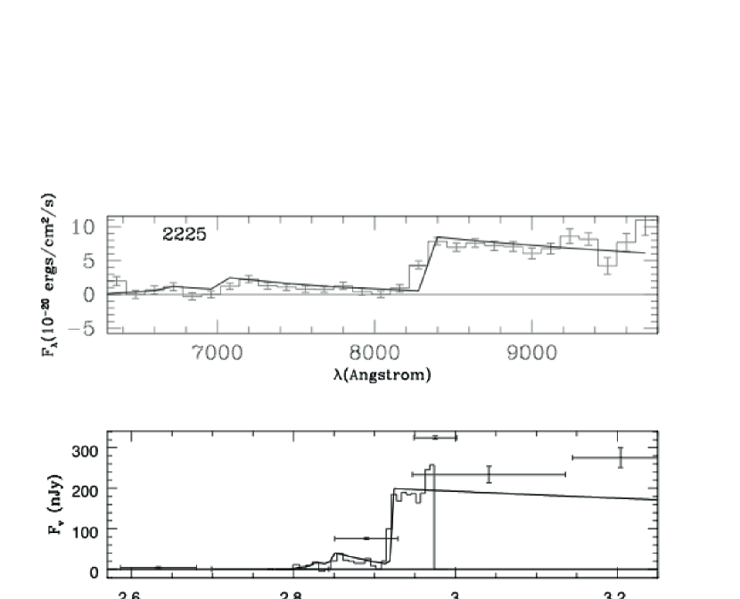
Figure 6: In this figure we present the grism spectra and the best fit using IGM absorption; the top panel show the fits in $F_{\lambda}$ vs. wavelength. The middle panel show the same objects in $F_{\nu}$ vs. log of wavelength, showing also the consistency with broad-band colors. The bottom panel shows cutout images ( 3arcsec on the side) in B,V, $i_{775}$, $z_{850}$, F110W and F160W. The stretch is each image is adjusted to go from -3$\sigma$ to 5$\sigma$. The top panel is labeled with the object name Due to size restrictions not all the spectra could be accomodated in the astro-ph version. Please go to www.stsci.edu/$\sim$san/spectra.pdf for a supplement that shows all the spectra

Twenty three galaxies are identified as high redshift galaxies on the basis of their spectra. This identification is based on detecting the Lyman break in the continuum for 22 of these sources and Lyman-$\alpha$ line and break in one source. For sources as bright as UDF2225, identifying a Lyman break is unambiguous (see Figure 6 for this spectrum). For most other galaxies the signal-to-noise ratio is low, and thus the following procedure was adopted to select reasonable spectral confirmations. The spectra were fit with a Lyman break galaxy template with a power law spectrum of slope $\alpha=0.2$ (where $f_{\nu}\propto\nu^{\alpha}$) attenuated by IGM absorption calculated according to the prescription of Madau 1995. We do a grid search on the parameters redshift and flux at 1250 Å to determine the best fit. With the low s/n, the $\chi^{2}$ per degree of freedom is generally less than 1 . For the sources to be identified as high redshift galaxies we require that (A) the chi-square per degree of freedom be about one; (B) the combined flux redward of the break is well detected, with net $s/n\geq 3$; and (C) the broad-band fluxes are consistent with the grism flux and the fitted LBG spectrum, even though we do not fit to broad-band fluxes while determining redshifts. With regard to point (C) we tolerate about 30% discrepancy in the flux between broad-band and grism measurements, because the aperture match between imaging and the grism often results in discrepancies of that order.

3 Comparison with color selection

Figure 1: The identity of complete color selected sample in the Hubble Ultra Deep Field is shown in this color magnitude plot, the axes of which span the color and magnitude range considered here. labels ’Z’ indicate high redshift galaxy, ’S’ a star, and E indicates an ERO type of galaxy. Small dots denotes galaxies for which we did not have enough data to identify them, either because the galaxies fell outside the GRAPES field, or because of overlap and contamination by other spectra.

Among the 29 objects that we have examined to have clean (non-contaminated), relatively high S/N spectra, 23 are high redshift galaxies. This implies about 80% chance of finding a high redshift galaxy with a color selection of ($i_{775}$-$z_{850}$) $>0.9$. The five galaxies with spectral shapes indicating old or reddened populations at medium redshifts have colors of ($i_{775}$-$z_{850}$)$\approx 1.0$. Thus a color cut of ($i_{775}$-$z_{850}$) $\approx 1.3$ adopted by Yan and Windhorst 2004 and by Bunker et al. 2004 is succesful at eliminating moderate redshift galaxies. The M-dwarf stars identified spectroscopically have ($i_{775}$-$z_{850}$) colors similar to the high redshift galaxies, but are not as faint (Pirzkal et al. 2005). Figure 1 shows the color magnitude distribution of the spectroscopically confirmed high redshift galaxies, stars, and moderate redshift red galaxies.

In Figure 2 we plot the ($i_{775}$-$z_{850}$) color of the spectroscopically confirmed galaxies against the redshift found by fitting a Lyman-break galaxy template. Superposed on that distribution is the expected color for star-forming galaxies from Bruzual & Charlot 2003 models with stellar population ages of 1,10,100 and 1000 Myrs assuming constant star-formation models with solar metallicity. We see that the observed color-redshift distribution follows the theoretical curves reasonably. This is not suprising, since the main effect determining the ($i_{775}$-$z_{850}$) color is the shifting of the Lyman break to longer wavelengths with redshift. There are color variations in the galaxies and some are bluer or redder than the models. The scatter in colors seen is larger than the models would indicate, but are not more deviant than $3\sigma$ in the color errors. The redder than expected color can be explained by invoking dust. The bluer color could be due to the presence of Lyman-$\alpha$ line emission which is not distinctly seen due to the low resolution of the spectra, but can make ($i_{775}$- $z_{850}$) bluer for galaxies upto $z=6$. Some of the apparent color scatter may be due to systematic errors in photometry due to the presence of neighbours. There is also an intrinsic color variation seen in two pairs of sources (3377/3398 and 3317/3325). Both pairs are resolved into separate objects in the official HUDF catalog but have the same redshift based on the break seen in the spectra. The difference in the ($i_{775}$- $z_{850}$) color is 0.7 magnitudes for the 3317/3325 pair and 0.4 magnitudes for the 3377/3398 pair. This shows that there is likely to be a fair variation of ($i_{775}$- $z_{850}$) colors within the same object. Whatever the reason for the color scatter, Figure 2 shows that it would lead to 20-30% incompleteness with the ($i_{775}$-$z_{850}$)$>1.3$ cut for $z\approx 6$ galaxies (YW04, Bunker et al. 2004).

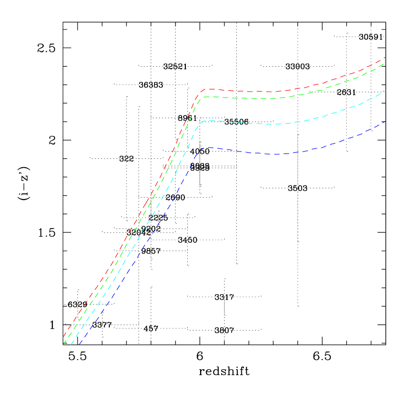
Figure 2: The ($i_{775}$-$z_{850}$) colors of galaxies are plotted against the redshift determined from grism spectra. The agreement with the theoretical curves is generally good, although we see a bias towards slightly blue colors, that might be due to the presence of Lyman-$\alpha$ line.The curves show colors of galaxies vs redshift using Bruzual & Charlot models of ages $10^{6}$, $10^{7}$,$10^{8}$,$10^{9}$ years going from bottom to top (or blue to red).

4 Overdensity at $z=5.9\pm 0.2$

Figure 3 shows the redshift distribution of the spectroscopically confirmed galaxies. We see an overdensity at $z=5.9\pm 0.2$. An overdensity was suggested by Stanway et al. (2004) on the basis of three galaxies in and near the UDF. We see it confirmed here, with 15 galaxies in the redshift range instead of 6 expected from the lower and higher redshifts in this sample. Thus the overdensity is 3.5 $\sigma$, assuming Poisson statistics. Doing the most naïve and straightforward estimate, we find that about 2/3rd of the galaxies in the sample are in 1/3rd of the volume, implying an overdensity of a factor of four.

Figure 3: The redshift histogram of galaxies. We see a definite overdensity at $z=5.9\pm 0.2$. Superposed on the histogram are curves of expected numbers of galaxies in these bins. Toward the high redshift bins the expected numbers fall off due to lack in sensitivity. In the low redshift regime the expected number of objects drops because the color selection misses the bluer objects. The solid lines show the expected numbers of objects with spectra like the Bruzual and Charlot 2003 models with reddening of E(B-V)$=0.15\pm 0.15$, for a range of 1(lower, blue curve) and 1000 (upper, red curve) Myrs old stellar populations. The dashed lines show the expected numbers if the objects have the color range seen at $5.7\leq z\leq 6.1$ in our sample.

This overdensity cannot be explained by selection effects alone. In Figure 3 we over-plot the expected number density of objects. Folding in the color selection, the grism response function and a Lyman break galaxy luminosity function from YW04, we predict the number of galaxies in each redshift bin, shown in figure 3. The drop-off at the higher redshift is due to a decline in the sensitivity of the grism at the red end, the roll-off at the low redshift in the models is due to the color selection, which starts to make us lose the bluer end of the z=5.5 sample. The solid curves show selection function with the color variation introduced by supposing a reddening with mean E(B-V)=0.15 magnitudes and $\sigma(E_{(B-V)})=$ 0.15 magnitudes, which is standard for Lyman break galaxies (Giavalisco, private comm.); the underlying stellar populations are 1 and 1000 Myrs old for the two curves. The dashed curves show the selection function at z=5.5 if we use the wider color range empirically seen in our sample at z=5.7-6.1. In the end the total number of i-drops matches the YW04 number and the overdensity at z=5.9 is seen to be a factor of 2. Thus a factor of two is the conservative lower bound on the peak at overdensity at $z\approx 6$, averaged over the field of view.

The true overdensity could be higher if the peak is substantially spread out by low redshift resolution in the grism data. With the low resolution spectra afforded by the ACS Grism, we are able to determine the redshifts to an accuracy of $\Delta z\approx 0.15$ for a typical object of size 0.”25. Besides this, Lyman-$\alpha$ emission can bias the redshift measurements obtained from the Lyman break, even if the line is too weak to appear obvious in the low-resolution grism spectrum. The shift in the estimate is described by $(\exp{(-EW/\sigma)}-1)\times\sigma$ where $2.355\sigma$ is the FWHM resolution of the spectrum. For typical values in the GRAPES survey, this corresponds to a shift of $\lesssim 200$Å, or a redshift change of $\lesssim 0.15$. This implies that $\Delta z=0.15-0.2$. So any spike in the distribution of galaxies is smeared by up to $\Delta z=0.2$ due to the limited wavelength resolution of the grism.

The overdensity at z=5.9 is also supported by complementary data on Lyman-$\alpha$ emitters from CTIO by Wang, Malhotra & Rhoads (2005) who have imaged a large area, 36’ $=12.9$ Mpc on a side, including the Hubble Ultra Deep Field. They show that the HUDF sits on the edge of a much larger scale ($>3$ Mpc) structure traced by Lyman-$\alpha$ emitters at z=5.7-5.77. Wang et al. 2005 report roughly a factor 3-4 overdensity in the Lyman-$\alpha$ emitters at z $\approx 5.8$, compared to other studies of Lyman-$\alpha$ emitters at z=5.8 (Rhoads et al. 2003, Rhoads & Malhotra 2001, Hu et al. 2003, MR04).

Figure 4 shows the distribution in the sky of the 15 galaxies in the redshift range $z=5.9\pm 0.2$ in the HUDF along with the larger scale structure seen in the Lyman-$\alpha$ emitters at z=5.7-5.77. We see that the galaxy distribution in the HUDF continues the voids seen in the larger distribution. Even within the HUDF the $z\sim 6$ galaxies are not distributed uniformly, and avoid one corner of the field. We applied a two dimensional Kolmogrov-Smirnov test (Peacock 1983, Fasano & Franceschini 1987, Press et al. 1992) to the distribution of the 15 galaxies at $z=5.9\pm 0.2$. Even with just 15 galaxies, the test gives only a 5% chance that they could be so arranged due to chance. Large scale structure has been seen in several such studies for both Lyman Break galaxies and Lyman-$\alpha$ emitters (e.g., Steidel et al. 1998, 2000; Venemans et al. 2002; Miley et al. 2004; Palunas et al. 2004; Ouchi et al. 2001, 2003; Shimasaku et al. 2003; Foucaud et al. 2003; and references therein).

Figure 4: (A) This figure shows the placement in the sky of the $z\sim 6$ galaxies in the UDF - seen here as square points in the diamond inset which is the UDF coverage. The $z\sim 6$ galaxies avoid the eastern corner of the UDF. A two-dimensional KS test shows that the probability of this configuration by chance is about 5%. A larger scale structure is seen in the Lyman-$\alpha$ emitters at z=5.7-5.77 which is consistent with the UDF structure. The dotted rectangle shows the area not covered by the Lyman-$\alpha$ survey due to a dead chip in the MOSAIC camera at CTIO.(B) shows the placement of galaxies at $z=5.9\pm 0.2$ in the HUDF, (the left hand) half of the chip is devoid of galaxies.

4.1 Expectation of overdensity

The location of the Hubble Ultra Deep Field was selected to include a reasonably bright known galaxy at z=5.8 found in the GOODS survey (Dickinson et al. 2004). Given that, we should consider what sort of overdensity is expected. We calculate the overdensity in the galaxy abundance in a cylindrical volume centered around a massive central galaxy.

The first step is to compute the halo mass of the central galaxy. The total mass of a halo that corresponds to the abundance of 1 object between $5.5<z<6.5$ in a solid angle of $\Delta\Omega=150$arcmin² is $M_{c}=9.1\times 10^{11}~{}{\rm M_{\odot}}$, which in turn corresponds to a $3.7\sigma$ peak in the density field. This assumes a duty cycle of $10^{8}$ yrs: each halo is assumed to be visible only a fraction $f_{d}=10^{8}{\rm yr}/t_{H}(z=5.9)=0.11$ of the time, where $t_{H}(z)$ is the age of the universe. The background cosmology is assumed to be flat $\Lambda$CDM with $\Omega_{\rm m}=0.29$ and $H_{0}=72~{}{\rm km~{}s^{-1}~{}Mpc^{-1}}$, consistent with the recent WMAP measurements (Spergel et al. 2003). The halo mass function was taken from the fit to numerical simulations in Jenkins et al. 2001.

The second step is to estimate the typical expected galaxy overdensity in the observed volume. The volume is taken here to be a cylinder centered at $z=5.9$ with angular diameter 3’ (or $2R=7$ comoving Mpc at $z=5.9$) and extending over the redshift range $z=5.9\pm 0.2$ (corresponding to a length of $2D=170$ comoving Mpc).

The mean overdensity $\langle\delta_{g}\rangle$ of galaxies of mass $M_{s}$ expected to fall within this cylinder can then be found by integrating the correlation function over the cylinder:

$$\langle\delta_{g}\rangle=\frac{1}{\pi(R^{2}-R^{2}_{\rm min})(D-R_{\rm min})}\times\int_{R_{\rm min}}^{R}2\pi rdr\int_{R_{\rm min}}^{D}dD\left[1+b_{c}b_{s}g^{2}(z)\xi_{m}(x)\right].$$ (1)

Here $g(z)$ is the linear growth function, $b_{s}$ and $b_{c}$ are the linear halo bias (mw96, ) of the “satellite” and central halos with mass $M_{s}$ and $M_{c}$ respectively, $R_{\rm min}$ is a low-radius cut, which we take to be the sum of the virial radii of the $M_{s}$ and $M_{c}$ halos (in practice, the value does not matter), $\xi(r)$ is the 3D correlation function, and $x\equiv\sqrt{R^{2}+D^{2}}$ (the $\xi(r)$ subscripts $g$ and $m$ refer to the values for galaxies and dark matter respectively.

We find $\langle\delta_{g}\rangle=1.78$ for $M_{s}=M_{c}=9.1\times 10^{11}~{}{\rm M_{\odot}}$. This suggests that a factor of $\sim$two overdensity should be typical in the observed volume. We note that this overdensity is entirely a result of the high bias ($b=8.1$) of the massive halos. As a result of the long redshift extent of the overdense region (an order of magnitude larger than the correlation length of $\sim 10$ Mpc), the corresponding mass overdensity ($1+b^{2}\langle\delta_{m}\rangle\approx 1+\langle\delta_{g}\rangle$) is negligibly small, $\langle\delta_{m}\rangle=1.012$. If we assume that the redshift extent is reduced by a factor of 2 or 10 (changing $D$ from 85 Mpc to 42.5 or 8.5 Mpc), then we find $\langle\delta_{g}\rangle=2.5$ and 6.3, respectively. Thus higher resolution spectra may see a more dramatic overdensity.

Three-dimensional effects can clearly be relevant. The above results should motivate a study of the probability of intersecting the cosmic filamentary density distribution in a way to reveal an elongated overdense region with a large aspect ratio.

5 Discussion and conclusions

This paper establishes the fraction of color selected objects that are bona fide high redshift galaxies to be around 80% for the color $(i-z)>0.9$ and magnitude limit of z=27.1–27.5. For a color selection of $(i-z)>1.3$ and magnitude limit of $z^{\prime}<27.5$ mag, the success rate is 14/15, but such a color selection misses five blue objects that are at redshifts $z\approx 6$.

An overdensity is seen in the redshift distribution at $z=5.9\pm 0.2$. The galaxy number density in this redshift range is a factor of two to four high. The extent of the redshift range spanned by this overdensity may be smaller, because the grism spectra give redshifts for LBGs accurate only to $\Delta z\approx 0.15$. Lyman-$\alpha$ line emission and absorption may further increase the observed scatter. Hence the overdensity may be even larger in a small volume. Hints of such an overdensity were seen by Stanway et al.(2003), who found three Lyman-$\alpha$ emitters at $z\approx 5.9$ in their spectroscopic followup. One of their objects is the same as object number 2225 in our sample. Further, higher resolution spectroscopy would be invaluable in determining the exact redshift extent and structure of this overdense region. A search for Lyman-$\alpha$ emitters has shown an overdensity at z=5.77 (823 nm) relative to z=5.70 (815 nm) (Wang, Malhotra & Rhoads 2005), as well as a strong spatial gradient. The Hubble Ultra Deep Field sits at the edge of this overdensity at z=5.77, and judging by the redshift histograms seen in figure 3, is part of it. If we naively multiply the spatial extent ($\approx 12^{\prime}$) of the structure at z=5.77 seen by Wang et al. 2005 and the redshift extent ($\delta z=0.4$) of the overdensity seen in this paper, we would conclude that the overdensity spans a volume of comoving $1.5\times 10^{5}Mpc^{3}$. According to current theories it would be hard to produce a net overdensity of a factor of 4 over such a large volume, while an overdensity of two could be due to the presence of a bright galaxy in the UDF.

The overdensity at z=5.7-6.1, combined with a simple selection function afforded by the grism, gives us an opportunity to derive the luminosity function and star-formation rate in such an overdensity. The complicating factor is the incompleteness in the spectroscopic sample. As mentioned in section 2.1, we do not have spectral information for 17 out of 46 objects brighter than $z_{850}$ of 27.5. We can, however bracket the parameters of the luminosity function by assuming that the spectroscopically confirmed sample represents the lower limit and the upper limit is obtained by adding to that all the objects for which we have no information. Figure 5 shows the luminosity function for these two cases in the redshift range $Z=5.9\pm 0.2$ and the best fitting Schecter functions. Following Yan and Windhorst (2004), we assume a slope of $\alpha=-1.8$ and derive parameters ${m_{\star}}(z_{AB})=25.2$ and ${\phi_{\star}}$$=2.5\times 10^{-4}$. These values are comparable to the YW04 luminosity function for $\alpha=-1.8$ which is ${m_{\star}}(z_{AB})=25.7$ and ${\phi_{\star}}$$=4\times 10^{-4}$. While ${\phi_{\star}}$and ${m_{\star}}$have correlated error when fitting only upto $z_{850}$$=27.5$, the integrated star-formation is fairly robustly estimated. The star-formation rate density (SFRD) derived from integrating over the luminosity function of the spectroscopically confirmed sample is $2.5\times 10^{-2}M_{\odot}Mpc^{-3}year^{-1}$, following the UV to SFR conversion in Madau, Pozetti & Dickinson (1998). Correcting for completeness with a factor of 1.6 gives $4\times 10^{-2}M_{\odot}Mpc^{-3}year^{-1}$. All these values are significantly higher than YW04 value of $1.2-1.5\times 10^{-2}M_{\odot}Mpc^{-3}year^{-1}$, consistent with there being an overdensity of at least a factor of two in this redshift range. The lower bound to the SFR is obtained by summing up the UV luminosity in the objects spectroscopically confirmed and normalizing by the volume, which is simply calculated as the comoving volume between $Z=5.7-6.1$. Thus the minimum SFR=$1.0\times 10^{-2}M_{\odot}Mpc^{-3}year^{-1}$ which is twice the estimate of Bunker et al. 2004 from the same field. Correcting for spectroscopic incompleteness leads to SFR=$1.9\times 10^{-2}M_{\odot}Mpc^{-3}year^{-1}$ which comes close to the required SFR needed for driving reionization especially if there are metal poor stars in these galaxies and the IGM has a higher temperature (Stiavelli et al. 2004). The volume calculations above have taken the whole area of the HUDF, whereas on the plane of the sky $z\approx 6$ objects occupy about half (or less than) the area of the ACS chip (Figure 4). Thus the volume over-density is a factor of four and the local SFR in the overdensity is definitely enough to drive reionization of the local IGM.

By comparing with the luminosity function of Lyman-$\alpha$ emitters, we see that the space density normalization of LBGs in the UDF as measured here and by Yan and Windhorst ${\phi_{\star}}$$=2.5-4\times 10^{-4}$) is two to four times higher than that of Lyman-$\alpha$ emitters for which MR04 derive ${\phi_{\star}}$$=1\times 10^{-4}$ at z=5.7. The Lyman-$\alpha$ luminosity function derived by MR04 is based on many surveys in different parts of the sky, and therefore should be robust to cosmic variance. Given the overdensity estimates of a factor of 2-4 here, the difference between ${\phi_{\star}}$of the UDF LBGs and Lyman-$\alpha$ galaxies is not significant. The LBG space density could be consistent with that of Lyman-$\alpha$ emitters at z=5.7. That does not mean that every LBG has Lyman-$\alpha$ emission, or that there is a one-to-one correspondence between the two. That is because we often do not know the continuum luminosity of the Lyman-$\alpha$ galaxies, and they could be fainter than even this sample in the rest UV. On the flip side many of the LBGs in the present sample could have weak Lyman-$\alpha$ emission which would not be detected in low resolution spectra.

The SFRD derived from Lyman-$\alpha$emitters is $1.8-3.6\times 10^{-3}$, which is roughly a tenth of the SFRD derived here. This is consistent with the fact that SFR for individual Lyman-$\alpha$ galaxies, derived from the Lyman-$\alpha$ line alone, is on the average 1/10th that of a typical LBG (Rhoads et al. 2000, 2003, Dawson et al. 2004).

Figure 5: The solid points show the luminosity function of the spectroscopically confirmed galaxies in the redshift range z=5.7–6.1 where an overdensity is seen; and the solid line as the best fit Schecter function, assuming a faint end slope of $\alpha=-1.8$) giving the best fit values of (${\phi_{\star}}$, ${L_{\star}}$)=(25.2, 2.5$\times 10^{-4}$). The open circles show the data corrected for incompleteness of the spectroscopic sample, by adding the unidentified objects to the appropriate magnitude bin. The resulting parameters are (${m_{\star}}$, ${\phi_{\star}}$, $\alpha$)=(25.9, 4$\times 10^{-4}$,-1.8)

This sample of spectroscopically confirmed Lyman break galaxies can also provide an independent test of reionization. If the IGM is neutral at $z>6$, the fraction of Lyman break galaxies that show Lyman-$\alpha$ line emission should drop, because the damping wings of neutral IGM reduce the line to at most 1/3rd its original strength (Haiman 2002, Santos 2004). Prior to this paper, all the spectroscopically confirmed galaxies at $z>6$, and all but two at $z>5$, showed Lyman-$\alpha$ emission. This may be a selection effect, since objects with strong lines are easier to confirm spectrocopically. For reference, only 25% of LBGs show Lyman-$\alpha$ emission at $z\simeq 3$ (Steidel et al. 1999). Now we have a sample of about 23 Lyman break galaxies (LBGs) selected using low resolution spectra from the grism on HST at redshifts $z=5.4$–$7$, not biased by the presence or absence of Lyman-$\alpha$ line. Deep, higher-resolution spectra of these objects should be able to detect lines with rest-frame EW of 30 Å. This would determine the Lyman-$\alpha$ emitter fraction and thus constrain whether the IGM is neutral.

Appendix A Grism Spectra

In this appendix we present the grism spectra of 23 high redshift objects. On each, we superpose the best fit Lyman break spectrum , represented by a power law of $F_{\lambda}\propto\lambda^{2.2}$ and Madau IGM absorption (Madau 1995) (top panel). We also see a consistency with the broad-band fluxes (middle panel). The agreement with the broad band fluxes is not perfect due to aperture mismatches, which we have tried to minimize and because the broad-band fluxes were not used in fitting, and the UV slope of the galaxies does vary from object to object, unlike the models we have used. The quality of the data, the s/n seen in most sources, and the limited wavelength range redward of the Lyman break simply did not support fitting the slope as an extra parameter.

The error-bars on the near-infrared fluxes were estimated by placing random apertures of a range of sizes on the finished image and estimating the noise properties of those apertures. The error-bars calculated this way are larger than the typical errors quoted elsewhere (Bouwens et al. 2004), but reflect a more realistic picture. A similar exercise with ACS images gave error estimates that are similar to the formal error estimates obtained by multiplying the rms deviations with the square-root of the number of pixels.

Figure 7: (a) Spectra of (i’-z’) selected red objects, for which the spectra do not show a break but a steady rise of flux into the red. Some of these are old, elliptical galaxies ( UDF 8238 is further discussed by Daddi et al. 2005); and some may be dusty, star-forming galaxies

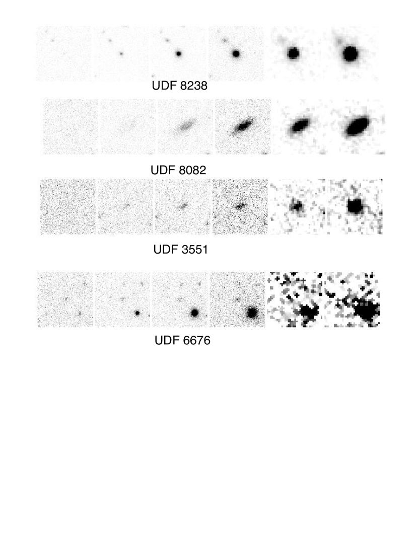
Figure 8: (b) Multiband images of color ($i_{775}$- $z_{850}$)$>0.9$ selected red objects, for which the spectra do not show a break but a steady rise of flux into the red. Some of these are old, elliptical galaxies ( UDF 8238 is further discussed by Daddi et al. 2005); and some may be dusty, star-forming galaxies. The images are $3"\times 3"$ on the side and are (going left to right) in the bands B,V,$i_{775}$,$z_{850}$, F110W( $\approx$ J band) and F160W ($\approx$ H band)

Table 1: Spectroscopic redshifts of i-droputs

UDF id	$z_{850}$	$i_{775}$-$z_{850}$	Redshift	RA (J2000)	DEC(J2000)	S/N
2225	25.06	1.55	5.8	03:32:40.012	-27:48:14.97	23.4
9202	27.43	1.56	5.7	03:32:33.207	-27:46:43.26	6.4
2690	27.33	1.7	5.9	03:32:33.781	-27:48: 7.59	7.0
32521	26.82	2.4	5.9	03:32:36.626	-27:47:50.06	6.7
3377/3398	26.49	1.0,1.3	5.6	03:32:32.636	-27:47:54.30	6.2
9857	26.95	1.4	5.8	03:32:39.066	-27:45:38.75	6.3
6329	26.88	1.1	5.5	03:32:35.196	-27:47:10.08	5.4
8961	26.54	2.12	5.8	03:32:34.097	-27:46:47.23	5.3
8033	26.05	1.9	6.0	03:32:36.467	-27:46:41.44	5.2
32042	28.2	2.4	5.75	03:32:40.554	-27:48: 2.61	4.9
36383	28.0	3.0	5.8	03:32:40.249	-27:46: 5.18	4.8
457	28.0	1.0	5.8	03:32:39.048	-27:49: 8.30	4.6
4050	27.33	1.9	6	03:32:33.429	-27:47:44.86	4.5
322	26.91	1.9	5.7	03:32:41.187	-27:49:14.85	3.9
3317	26.94	1.15	6.1	03:32:34.556	-27:47:55.15	4.3
3503	27.7	1.7	6.4	03:32:34.306	-27:47:53.54	4.3
3807	27.73	0.97	6.1	03:32:34.976	-27:47:48.05	3.9
3325	27	1.85	6.0	03:32:34.547	-27:47:55.98	3.7
3450	27.05	1.5	5.9	03:32:34.283	-27:47:52.35	3.4
35506	27.46	2.8	6.15	03:32:39.860	-27:46:19.08	3.1
33003	27.8	3.3	6.4	03:32:35.056	-27:47:40.18	3.3
30591	27.13	2.56	6.7	03:32:37.277	-27:48:54.57	3.5
Marginal detections
2631	27.71	2.262	6.6	03:32:42.596	-27:48: 8.83	2.9
Red galaxies at intermediate redshifts
8238, 8082, 3551, 1238, 6676
Dwarf stars
443, 366

References

- (1) Barger, A. J., Cowie, L. L., Capak, P., Alexander, D. M., Bauer, F. E., Brandt, W. N., Garmire, G. P., & Hornschemeier, A. E. 2003, ApJ, 584, L61
- (2) Becker, R. H. et al. 2001, AJ 122, 2850
- (3) 2003MNRAS.344.1000B Bruzual, G. & Charlot, S. 2003, MNRAS, 344, 1000
- (4) Bouwens, R.J., Thompson, R.I., Illingworth, G., Franx, M., van Dokkum, P., Fan, X., Dickinson, M., Eisenstein, D.J., Rieke, M., 2004, astroph-0409488.
- (5) Bunker, A J.; Stanway, E R.; Ellis, R S.; McMahon, R G., 2004, MNRAS, to appear, astro-ph/0403223
- (6) Daddi, E., Renzini, A., Pirzkal, N., et al. 2005, submitted to the ApJ.
- (7) Dickinson, M., et al. 2004, ApJ, 600, L99
- (8) Dijkstra, M., Haiman, Z., & Loeb, A. 2004, ApJ, 613, 646
- (9) Fan, X., Narayanan, V. K., Strauss, M. A., White, R. L., Becker, R. H., Pentericci, L., & Rix, H.-W. 2002, AJ 123, 1247
- (10) Giavalisco, M. 2002, ARA&A, 40, 579
- (11) Hu, E. M., Cowie, L. L., McMahon, R. G., Capak, P., Iwamuro, F., Kneib, J.-P., Maihara, T., Motohara, K. 2002, ApJ 568, L75
- (12) Hu, E. M., Cowie, L. L., , Capak, P., McMahon, r. g., Hayashino, T., & Komiyama, Y. 2004, AJ, 127,563.
- (13) Jenkins, A. et al. 2001, MNRAS, 321, 372
- (14) Madau, P. 1995, ApJ, 441, 18
- (15) Malhotra, S., Rhoads, J.E. 2004, ApJL, accepted (astro-ph/0407408)
- (16) Mo, H. J., & White, S. D. M. 1996, MNRAS, 282, 347
- (17) Moustakas, L.A., Immler, S. 2004, ApJL, submitted, astro-ph/0405270
- (18) Pirzkal, N., Pasquali, A., Demleitner, M., 2001, ST-ECF Newsletter, 29, “Extracting ACS Slitless Spectra with aXe, p. 5 (http://www.stecf.org/instruments/acs) ApJS 154, 501-508.
- (19) Pirzkal, N., Xu, C., Malhotra, S. et al. 2004,
- (20) Pirzkal, N., Sahu, K., et al. 2005, submitted to ApJ.
- (21) Press, W.H., Schechter, P, 1974 ApJ,187,425
- (22) Rhoads, J.E., Xu, C., et al. 2004 ApJ, 611,59
- (23) Shimasaku, K. et al. 2003, ApJ, 586, L111
- (24) Spergel, D. N., et al. 2003, ApJS, 148, 175
- (25) Stanway, E. R., et al. 2004, ApJ, 604, L13
- (26) Stiavelli, M., Fall, S. M., & Panagia, N. 2004, ApJ, 610, L1
- (27) Steidel, C. C., Pettini, M., & Hamilton, D. 1995, AJ, 110, 2519
- (28) Taniguchi,Y., Ajiki, M., Nagao,T., Shioya, Y., Kashikawa, N., Kodaira, K., Kaifu, N. et al, astroph-0407542.
- (29) Thompson, R. et al. 2005, Subimtted, AJ.
- (30) Wang, J. X., Malhotra, S., Rhoads, J. E., & Norman, C. A. 2004, ApJ, 612, L109
- (31) Wang, J. X., Malhotra, S., Rhoads, J. E., 2005, submitted to ApJ.
- (32) Yan, H.J., Windhorst, R., 2004, ApJ, 612, L93