Peering through the OH-forest: a new technique to remove residual sky features from SDSS spectra

Abstract

The Sloan Digital Sky Survey (SDSS) currently provides by far the largest homogeneous sample of intermediate signal-to-noise ratio (S/N) optical spectra of galaxies and quasars. The fully automated SDSS spectroscopic reduction pipeline has provided spectra of unprecedented quality that cover the wavelength range $3800-9200\,$Å. However, in common with spectra from virtually all multi-object surveys employing fibres, there remain significant systematic residuals in many of the spectra due to the incomplete subtraction of the strong OH sky emission lines longward of $6700\,$Å. These sky lines affect almost half the wavelength range of the SDSS spectra, and the S/N over substantial wavelength regions in many spectra is reduced by more than a factor of 2 over that expected from counting statistics. We present a method to automatically remove the sky residual signal, using a principal component analysis (PCA) which takes advantage of the correlation in the form of the sky subtraction residuals present in each spectrum. Application of the method results in spectra with essentially no evidence for degradation due to the incomplete subtraction of OH emission features. A dramatic improvement in the quality of a substantial number of spectra, particularly those of faint objects such as the bulk of the high-redshift quasars, is achieved. We make available IDL code and documentation to implement the sky residual subtraction scheme on SDSS spectra included in the public data releases. To ensure that absorption and emission features intrinsic to the object spectra do not affect the subtraction procedure line masks must be created that depend on the scientific application of interest. We illustrate the power of the sky-residual subtraction scheme using samples of SDSS galaxy and quasar spectra, presenting tests involving the near-infrared CaII triplet absorption, metal absorption line features in damped Ly$\alpha$ systems and composite spectra of high-redshift quasars.

1 Introduction

The development over the last two decades of efficient and reliable wide-field multi-object spectrographs has resulted in enormous advances in the ability to compile large samples of high-quality astronomical spectra. The Sloan Digital Sky Survey (SDSS; ?) represents the most impressive application yet of such an instrument to provide spectroscopic samples of quasars, galaxies and stars of unprecedented size. The third data release (DR3; Abazajian et al. 2004b) provides the astronomical community with nearly 500,000 object spectra and further releases will take the number to 750,000 within eighteen months.

The SDSS spectra present a dramatic improvement in quality over data from previous surveys: extended wavelength coverage, $3800-9200\,$Å; intermediate resolution, $\lambda/\Delta\lambda\simeq 2500$; high-quality relative and absolute flux-calibration; typical signal-to-noise ratios (S/N) of $10-30$; availability of accurate noise and mask arrays. Coupled with the overall homogeneity of the dataset this makes them suitable for an almost limitless number of quantitative investigations.

A particularly impressive aspect of the instrumental design, observing strategy and data reduction pipeline (?) has been the quality of the sky-subtraction achieved considering the relatively large, 3 arcsecond diameter fibres and fully automated reduction. Subsets of the SDSS spectra, such as the fainter quasars, include objects with magnitudes in red passbands equivalent to the sky-brightness per square arcsecond. Despite the demonstrable quality of the SDSS spectra, visual inspection reveals significant systematic sky-subtraction residuals longward of $6700\,$Å in many spectra. For fainter objects in particular, the sky-subtraction residuals are the dominant source of uncertainty over a wavelength interval of some $2000\,$Å. The spectroscopic region involved is extensive and includes features of significant astrophysical interest; examples include the Calcium triplet (8500, 8545, $8665\,$Å), a powerful diagnostic of stellar populations in low-redshift galaxies, and the H$\beta$ + [OIII] 4959, $5007\,$Å emission region in quasars and active galactic nuclei (AGN) in the redshift interval $0.4<z<0.8$.

With sufficient care (e.g. ?) it is possible to quantify the noise properties of the SDSS spectra in the red, allowing the statistical significance of features to be estimated reliably. However, the decrease in the S/N relative to that expected from counting statistics can be factors of 2-3. Coupled with the substantial fraction of the spectral range affected, many potential scientific investigations are compromised.

The sky-subtraction procedures incorporated in the SDSS spectroscopic pipeline are very effective, overcoming a number of the longstanding problems associated with wide-field multi-fibre observations. Brief details can be found in the Early Data Release paper (?, Sections 4.8.5 and 4.10.1) and information on calibration improvements for the Second Data Release (DR2) are given in Abazajian et al. (2004a). While the large area of sky, $7.1\,$ square arcseconds, observed through the fibre aperture exacerbates the problem of achieving accurate sky-subtraction, the origin of the dominant systematic residuals present in the SDSS spectra is not a preserve of fibre spectroscopy alone. Rather, the fundamental issue lies in the ability to remove OH emission features from spectra in which the line profiles are barely resolved. Combined with sub-pixel changes in the pixel-to-wavelength calibration between spectra, sharp residuals often remain.

?) provides a recent summary of the difficulties associated with accurate sky-subtraction in long-slit observations, presenting a highly effective procedure for removing the signature of even rapidly varying and poorly sampled emission line features. The technique described by Kelson is certainly not applicable to the extracted fibre spectra available as part of the official SDSS Data Releases and any improvement must rely on an alternative procedure. The sky-subtraction residuals arise from the subtraction of two essentially identical tooth-comb signatures that have been very slightly misaligned relative to one another leading to well-defined patterns (Fig. 1). This suggests a correction procedure that takes advantage of the correlations present in the wavelength direction, offering significant advantages over simply masking the affected pixels.

More specifically, we develop an approach for the removal of the dominant OH sky-subtraction residuals in the SDSS spectra based on principal component analysis (PCA). PCA (also called Karhunen–Loève transformation) is a well-established data reduction technique in astronomy, frequently applied to classification and reconstruction problems associated with large numbers of spectra of various types of object (e.g. galaxies: Connolly et al. 1995; Folkes et al. 1996; Madgwick et al. 2002, 2003; Yip et al. 2004a. Quasars: Francis et al. 1992; Yip et al. 2004b. Stars: Whitney 1983). The idea of employing PCA for sky-subtraction has been suggested by ?), who present a complex method to remove the sky signal without the need for concurrent sky observations. However, the scheme appears to have generated little interest, perhaps because of the ambitious goal of the technique and the targeting of observations in which sky spectra are unavailable. By contrast, we develop a much more specific application of the PCA technique to the SDSS DR2 spectra that results in an improvement by over a factor of 2 in the S/N of those pixels longward of $6700\,$Å  affected by OH sky lines, dramatically increasing the potential use of the red half of the SDSS spectra for a variety of scientific investigations. The technique is equally applicable to the spectra in the recent DR3 release. We adopt the same convention as employed in the SDSS and use vacuum wavelengths throughout the paper.

In Section 2 we present our method which is applied to SDSS galaxy and quasar spectra in Section 3. Section 4 uses subsets of the SDSS DR2 spectroscopic catalogue to demonstrate application of the method to various astronomical studies. The code and documentation with which to carry out the method on public release SDSS spectra is available on the web at http://www.ast.cam.ac.uk/research/downloads
/code/vw/.

Figure 1: Examples of poor OH sky emission line subtraction in SDSS sky-subtracted sky spectra. Note the well-defined patterns present, particularly the characteristic positive-negative residuals.

2 Method

Our overall approach is determined by the extent of the spectroscopic information provided in a SDSS public data release. The raw CCD exposures, typically 4 or 5 per spectroscopic plate, that make up the total exposure in each spectroscopic field are not available, precluding any attempt to improve the sky-subtraction on an exposure by exposure basis. However, the SDSS data releases do provide the final reduced spectra for both target objects and for the fibres allocated to blank sky regions employed to define the underlying spectrum of the night sky. These contain significant diagnostic information about the quality of sky subtraction for each spectroscopic plate.

For each observation of a SDSS spectroscopic plate, approximately 32 fibres, 16 for each of the 2 spectrographs, are assigned to blank sky regions, selected from areas containing no detected objects in the SDSS imaging survey. The sky fibres are identified as “SKY” in the catalogue’s “OBJTYPE” and “SPECCLASS” field. The sky spectra are combined to create a “master-sky” spectrum for each spectroscopic plate, which is then scaled and subtracted from each of the 640 spectra, producing 608 sky-subtracted object spectra and 32 sky-subtracted sky spectra, all of which are part of the standard SDSS data releases. Throughout the remainder of the paper we will refer to the sky-subtracted sky spectra as “sky spectra”, and the sky-subtracted object spectra as “object spectra”.

The availability of large numbers of sky spectra, over 18,500 in DR2, thus provides a direct empirical measure of the noise resulting from counting statistics as well as any systematic residuals from the sky-subtraction procedure. The scale of the SDSS releases is such that the application of empirical self-calibration techniques, based on the statistical properties of the data set itself, can be a powerful tool.

Visual inspection of the spectra of faint objects, or sky spectra (Fig. 1), immediately reveals the presence of “patterns” due to small imperfections in sky subtraction. The presence of systematic deviations that are correlated over extended wavelength ranges suggests that a technique capable of quantifying the form and amplitude of the correlated deviations could allow the removal of a substantial fraction of the sky-subtraction noise. PCA is a well-established technique with a number of desirable properties for such an application.

The principles behind our sky-subtraction method are simple to understand: a PCA of the sky spectra produces a set of orthogonal components that provides a compact representation of the systematic residuals resulting from the sky-subtraction process. The components are then added in linear combinations to remove the systematic sky residuals from the spectra of target objects, such as galaxies.

Our analysis focuses on the red part of the SDSS spectra ($6700-9180\,$Å), as the strong emission features blueward of $6700\,$Å  are small in number and easily masked. The upper limit of $9180\,$Å is set by the requirement that the entire wavelength region be included in all spectra when creating the PCA components from the sky spectra. Although techniques exist to overcome this (?), it was believed they would not greatly improve the applicability of the procedure for scientific objectives due to the very small fraction of plates affected.

2.1 A sample of sky spectra

The goal of the sky-subtraction scheme is to remove any systematic residuals from the bulk of the SDSS spectra. Pathological spectra with very unusual deviations can have a disproportionate effect on the generation of the PCA components. Therefore, we identify a restricted subset of the full 18,764 sky spectra for use in deriving the PCA components.

For the wavelength range used in the analysis ($6700-9180\,$Å) the spectra must satisfy the following criteria, where the numerical values are in the units of the SDSS spectra ($10^{-17}{\rm erg\ s^{-1}cm^{-2}\AA^{-1}}$):

1. $-0.2<$ mean flux $<0.2$, ensuring the spectra have a mean close to zero.

2. variance of the flux $<0.8$, ensuring that the amplitude of pixel-to-pixel fluctuations is not unusually high

3. “spectral colours” have values $|a-b|<0.1$, $|a-c|<0.3$ and $|b-c|<0.3$ ensuring that the spectra do not exhibit significant large scale gradients. $a$, $b$ and $c$ are calculated by averaging the flux in three wavelength regions largely free of OH sky emission (7000:7200 Å  [a], 8100:8250 Å  [b] and 9100:9180 Å  [c]).

We further only accept spectra with a minimum of 3800 good pixels (“NGOOD” parameter) over the entire wavelength range of the spectrum, to eliminate spectra with substantial numbers of missing pixels. Following a trial run of the PCA, 300 spectra are identified as outliers in the distribution of principal components, therefore dominating particular components, and discarded (see Section 2.2). Application of these selection criteria leaves 15,178  sky spectra. Finally, the spectra were normalised to have a median flux of zero over the wavelength range $6700-9180\,$Å. None of the results in the paper depend on the details of the criteria used to define the subset of sky spectra to be used in the PCA-analysis.

2.1.1 Poisson error normalisation

The true error on each pixel in each spectrum is made up of components due to Poisson noise and systematic sky-subtraction errors. Our method for removing sky residuals relies on determining the best-fit PCA-components via a minimum least-squares criterion over all pixels within the $6700-9180\,$Å  wavelength range. A pixel which varies greatly between spectra will be weighted highly during the generation of the PCA-components and in the subsequent reconstruction of the sky-residuals present in individual spectra. For example, there will be a greater variance among spectra at wavelengths in the vicinity of strong OH emission lines, purely due to Poisson noise and independent of whether there is a contribution due to sky-subtraction errors. It follows that to achieve effective sky-subtraction it is important to normalise each spectrum by the Poisson noise expected at each pixel. Failure to do so results in over-subtraction for certain pixels, with “corrected” pixels apparently exhibiting fluctuations below the Poisson limit.

Figure 2: Top: the flux rms (67th percentile) of the 15,178  sky spectra. Bottom: same as top, with the flux normalised by the associated median SDSS spectroscopic plate noise arrays. The impact of the presence of the OH sky emission lines is evident from the increase in the rms (by nearly a factor 2 at maximum), even after the empirical scaling of the noise arrays in the SDSS spectroscopic reduction pipeline.

Each SDSS spectrum includes a companion error array based on the original Poisson errors derived from photon counts, CCD read-noise and so forth. Unfortunately for our application, the error arrays have been systematically increased in regions of poor sky subtraction. The procedure is carried out separately for each plate and details can be found in the data reduction source code at http://spectro.princeton.edu/idlspec2d_doc.html#SKYSUBTRACT. Fig. 2 shows the flux standard deviation (rms) of the 15,178  sky spectra with and without normalisation by the associated SDSS noise arrays. If the SDSS noise arrays accounted for all the variance present in the spectra, the lower plot in Fig. 2 would be flat. In fact the SDSS noise arrays account well both for the increased “continuum” noise at red wavelengths, the presence of the atmospheric A-band at $\sim 7600$Å and the contribution from the increased sky emission associated with the presence of the broad O₂ airglow emission centred on $\sim 8650$Å. However, significant additional residual variance resulting from the incomplete subtraction of the barely resolved OH emission lines remains. For many applications the resulting scaled error arrays, which better reflect the true error in each spectrum, are an improvement. However, using the modified SDSS noise arrays for our sky-subtraction procedure does not allow it to reach its full potential, due to the excessive down-weighting of strong OH features.

It is not possible to recover directly the original Poisson errors that we require, so instead we develop an empirical approximation from investigation of several spectroscopic plates prior to sky subtraction, kindly made available to us by the SDSS project (E. Switzer, P. Macdonald and D. Schlegel). These data confirmed the expectation that scaling of the error arrays is applied by the SDSS reduction pipeline predominantly at positions of OH emission features. The same noise scaling is applied to all spectra on a plate, allowing us to derive a single rescaling for each plate. For each one of the 574 plates we calculate the median noise at each wavelength increment (pixel) from the SDSS error arrays of the sky spectra. The continuum noise is calculated over the full wavelength range of interest interpolating across pixels containing OH sky emission lines. The amplitude of this continuum noise is dominated by counting statistics, and rises towards the red (Fig. 2; upper panel) due to an increase in the sky level and instrumental effects.

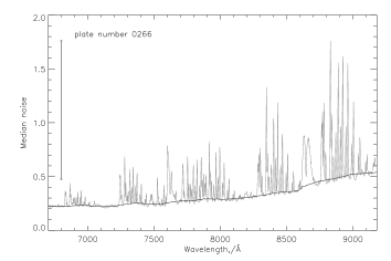
Figure 3: The median noise array for plate number 0266 (grey) and the estimated continuum overplotted (black). The bar to the left hand side indicates the amplitude of max$(n-c)$ for this plate, which occurs at the wavelength of $8829\,$Å.

We use a simple function to approximate the rescaling of the noise, $S_{i}$, for each pixel $i$ on each plate:

$$S_{i}=1+\left[\frac{(n-c)_{i}}{{\rm max}(n-c)}\right]^{\alpha}\times\beta$$ (1)

where $n$ is the median noise of the plate, $c$ the continuum noise, and max$(n-c)$ the maximum noise, above the continuum level, over all pixels. Fig. 3 shows an example plate median noise array, with estimated continuum and max$(n-c)$ marked. $\alpha$ and $\beta$ are determined empirically as described below and represent, respectively, the relative amount of rescaling between pixels with differing amounts of noise, and the total rescaling of the pixel with the highest noise above continuum level. As the exact effects of the SDSS noise scaling are not understood, the form of this function is chosen to provide flexibility in both the total rescaling and dependence with wavelength.

Figure 4: Top: the flux rms (67th percentile) of the 15,178  sky spectra. The lower (upper) spectrum is before (after) the sky-residual subtraction is performed. Bottom: same as top, with flux normalised by the associated median SDSS spectroscopic plate noise arrays, scaled according to Eq. 1 ($\alpha=1,\beta=0.3$). For clarity, the upper spectra have been displaced vertically by 2.5 units (upper panel) and 1.5 units (lower panel). The effectiveness of the sky-residual subtraction procedure is seen by the reduction by more than half of the systematic spikes in the top figure, and complete removal in the bottom figure.

Anticipating the results of Section 3, the effectiveness of the PCA sky-residual subtraction procedure can be seen in Fig. 4. The top panel shows the effect of the sky-residual subtraction on the raw rms of the sky spectra: the lower spectrum shows the uncorrected rms as a function of wavelength (reproducing the top spectrum from Fig. 2); the upper spectrum shows the raw rms after application of the sky-residual subtraction scheme. Note how the features due to the atmospheric A-band ($\sim 7600\,$Å) and O₂-emission ($\sim 8450\,$Å) are unaffected, while the height of the spikes associated with the OH emission lines is greatly reduced. The variation with wavelength of the rms, post sky-residual subtraction, is explained almost entirely by counting statistics. The bottom panel of Fig. 4 shows the rms of the sky spectra weighted by our modified noise arrays (with $\alpha=1,\beta=0.3$): the lower and upper spectra show the rms before and after subtraction of the sky residuals respectively.

Figure 5: Flux rms (67th percentile) of the 15,178  sky spectra after sky-residual subtraction is performed, with flux normalised by the associated median SDSS spectroscopic plate noise arrays, scaled according to Eq. 1. From bottom to top $\beta=0,0.1,0.2,0.3,0.4,0.5$ and $\alpha=1$.

Fig. 5 shows the effect of varying the noise rescaling ($\beta$ in Eq. (1)) applied to the sky spectra prior to creating the eigenspectra. From bottom to top $\beta=0,0.1,0.2,0.3,0.4,0.5$. For low values of $\beta$ (small amounts of rescaling of the noise arrays) the noise weighted rms is approximately constant with wavelength, i.e. the sky-residual subtraction procedure is not removing signal below the Poisson limit for any pixels, although the procedure may also not be removing the full systematic contribution to the errors. As beta increases, initially the rms remains constant until a point is reached where significant dips appear in the red half of the spectra. The presence of these dips show that an unphysical situation has resulted, where, following the rescaling, the noise falls below the Poisson limit for those pixels. The same effect is seen if we undertake the sky residual subtraction without weighting the flux by the noise arrays, i.e. the noise is constant, independent of wavelength. The fact that we can rescale the noise arrays by some amount before these unphysical dips appear, indicates that the SDSS noise arrays have indeed been scaled to take account of the presence of a systematic contribution to the noise at wavelengths where the OH-emission is significant.

Under-subtraction of the sky-residual signal due to over estimation of the Poisson errors prevents our sky-residual subtraction method from reaching its full potential. Over-subtraction of the sky-residual signal causes downward spikes to appear at the location of the OH emission lines (Fig. 5), as we begin to erroneously subtract Poisson noise. This suggests a simple method to estimate the values of $\alpha$ and $\beta$ in Eq. 1: we require the weighted flux rms, post sky-residual subtraction, to be as constant with wavelength as possible whilst maximising the noise rescaling. We take a grid of values for $\alpha$ and $\beta$ and for each combination first run the PCA on the 15,178  sky spectra with noise normalisation scaled according to Eq. (1), then perform with the sky-residual subtraction with the same noise weighting. By calculating the standard deviation of the rms array, post sky-residual subtraction, for each value of ($\alpha$, $\beta$) we can derive the best empirical rescaling of the SDSS noise arrays: we require the greatest value of $\beta$ that does not introduce upward or downward spikes, whilst $\alpha$ allows purely for potential wavelength variations. We find that $\alpha=1$ and $\beta=0.3$. Our final results are insensitive to small changes in $\alpha$ or $\beta$, and the measured value of $\alpha=1$ suggests that the empirical rescaling of the noise arrays within the SDSS spectroscopic pipeline is predominantly a function of the height of the OH spikes above the continuum noise. By systematically decreasing the amplitude of the noise arrays by 30% at positions of OH lines whilst retaining a constant noise weighted rms with wavelength, we substantially increase the effectiveness of the method, without over-subtracting residual sky features beyond the limit set by counting statistics.

We emphasise that it is not possible to derive the true noise array, based on counting statistics, for each SDSS spectrum from the information contained in the publically available SDSS data releases. However, the close to constant rms as a function of wavelength achieved following our empirical rescaling of the noise arrays (Fig. 4; bottom panel) is strong evidence that, while approximate, the scheme does achieve a highly effective correction, reducing the rms close to the level set by counting statistics at all wavelengths. If a version of our sky-residual subtraction scheme could be applied to the SDSS spectra using the true noise arrays, based on counting statistics, then further improvements should result.

2.1.2 Identification of sky pixels

The strong sky emission lines, which lead to the presence of systematic sky-residuals, occupy only a fraction of the $6700-9180\,$Å wavelength range and it is necessary to identify those pixels which suffer significantly from sky subtraction errors. The affected pixels can be found via the calculation of the rms of the 15,178  sky spectra, normalised by the corresponding SDSS noise arrays (as shown in the lower panel of Fig. 2). All pixels above a threshold value are defined as “sky pixels”. The “non-sky pixels” are not included in the PCA sky-residual removal procedure but provide an empirical estimate of the level of Poisson noise (i.e. excluding systematic sky-residuals) present in each spectrum. Adopting a threshold level of 0.85 for the sky/non-sky boundary, the scheme results in 670 sky pixels and 697 non-sky pixels. The results shown in subsequent sections are not sensitive to reasonable variations in the threshold level. Finally, to minimise their effect during the calculation of the PCA components, sky pixels in each spectrum where the associated SDSS noise array is zero (i.e. no data) are set to the mean value of the pixel in all the sky spectra that contain data.

2.2 Principal component analysis

Figure 6: From top to bottom, the first 5 sky principal components, each offset vertically from the next by a value 0.35. A horizontal dashed line indicates zero flux in each component.

PCA is a simple statistical method for data reduction which looks for components in a dataset that vary the most. The technique can be visualised by imagining an $M$-dimensional array, where $M$ is the number of pixels in the spectra. Each spectrum is then represented by a point in the $M$-dimensional array; PCA searches for lines of greatest variance through the array, each one being orthogonal to all previous lines. The line of greatest variance defines the first PCA component, and so on until the line of least variance defines the $M^{th}$ PCA component. The projection of an individual spectrum back onto a PCA component gives the amplitude of the component contained in that particular spectrum. A spectrum is reconstructed by summing the principal components multiplied by the relative amplitudes for that spectrum. Appendix A presents the mathematics of PCA.

Having created a sample of sky spectra containing only those pixels with sky signal and weighted by our empirically derived noise array for the relevant plate, we run the PCA. The output consists of $M$ principal components which are $M$ pixels long. Each component has an associated variance, which gives the percentage of the total variance of the dataset contained in that component.

As PCA can be sensitive to spectra with particularly unusual features in which we are not interested, we remove spectra which dominate the signal in individual components after one trial run. The pruning, of 300 spectra in total, is achieved by removing those spectra with principal component amplitudes more than $5\sigma$ from the mean. The PCA is then rerun on the resulting sample of sky spectra. Fig. 6 shows the first 5 principal components resulting from the analysis. Note the distinctive, correlated features present in each component.

Once the components are created, they can be used as templates to reconstruct the input sky spectra and later the sky residuals in the object spectra (Section 2.3). This is done by projection of each spectrum onto the components and summation of the components weighted by the projection coefficients (Eq. 6 and 6). The reconstruction may then be subtracted from the sky spectra leaving residual-free spectra, termed sky-residual subtracted spectra.

2.2.1 The number of components

The number of components to use in the reconstruction is not well defined. The use of too many results in the artificial suppression of noise below the Poisson limit, with the PCA acting as an (undesirable) high-frequency filter. The use of too few components means that the removal of sky residuals is sub-optimal and, in some cases, the overall quality of the spectra can decrease.

Fig. 7 shows the mean ratio of the rms of the noise-weighted flux in the sky pixels to that in the non-sky pixels, for the 15,178  sky-residual subtracted sky spectra, as a function of the number of components used in the reconstructions. The rms of the non-sky pixels in each spectrum remains constant and the ratio decreases monotonically as more components are used in the reconstructions, with an increasing fraction of the noise in the sky pixels removed.

The reduction of the noise in the sky pixels below the noise in the non-sky pixels is clearly unphysical, and we therefore estimate the number of components to employ in the reconstruction of each spectrum by adopting the non-sky pixel rms of that spectrum as a reference. The reconstruction of a spectrum proceeds one component at a time, with the rms ratio calculated for the sky-residual subtracted spectrum. Reconstruction is stopped when the rms ratio reaches unity, i.e. when the noise weighted flux rms is the same for the sky and non-sky pixels. The scheme is largely self-calibrating. For example, in spectra with high S/N the systematic sky residuals typically contribute only marginally to the sky-pixel noise, the rms ratio thus starts close to unity and only a small number of components are necessary to achieve equality in the rms ratio.

The large number of pixels that contribute, combined with the robust estimator of the non-sky rms, mean the amplitude of the non-sky rms is well determined, providing an excellent indicator of when to halt the reconstructions. Fig. 8 shows the distribution of the number of components used for DR2 sky, galaxy and quasar spectra. For bright objects the contribution to the noise from imperfections in the sky subtraction is small and few components are required to bring the sky and non-sky rms to the same level. The presence of many spectra with high S/N produces the “spike” at low component numbers in both the galaxy and quasar sample histograms. The fainter limiting magnitude of the quasar sample make sky-residuals a problem in a larger fraction of the spectra and, on average, more components are required to remove the systematic errors present following the default SDSS-pipeline sky-subtraction. To limit the effect of very occasional poor estimation of the non-sky rms we set the maximum number of components to 150 and 200 for the galaxy and quasar samples respectively.

Figure 7: The mean ratio of sky to non-sky flux rms over all sky spectra in our sample as a function of the number of components used during sky residual reconstruction. Fluxes are weighted by their respective scaled plate noise arrays. The horizontal dashed line indicates where the two rms values are equal. The error bars show the standard deviation of all objects in the sample.

Figure 8: Histograms showing the number of components used to reconstruct the sky signal in the sky (dotted line), galaxy (thin line) and quasar (thick line) DR2 samples. The y axis is truncated in order to show the majority of the objects, 18% (5%) of galaxies (quasars) require zero components.

2.3 Reconstructing sky residuals in an object spectrum

In the preceding sections we have developed a procedure that achieves a substantial reduction in the amplitude of the systematic sky residuals in spectra that possess no large scale signal, i.e. the successfully sky spectra are known, by definition, to possess zero signal at all wavelengths. We now turn to the more interesting application of removing the systematic sky-residuals from the SDSS science spectra of targets such as galaxies and quasars.

The problem is made tractable by the success of the sky-subtraction procedure performed as part of the standard SDSS spectroscopic pipeline. Detailed examination of the properties of the sky spectra shows that both the mean level and the large scale shape of the sky spectrum to be subtracted from each spectrum have been determined to very high accuracy. As a result, there is effectively no sky “continuum” to remove, rather the problem is confined to removing the high-frequency structure due to the presence of the strong OH sky emission lines. The key goal is to ensure that object continuum and intrinsic absorption and emission line features are not removed as a result of the procedure used to reduce the amplitude of the systematic sky-residuals.

As it is not necessary to identify any sky continuum present, we can remove the continuum of the object spectrum using a median filter before projection of the spectrum onto the principal components derived from the sky spectra. The smallest filter size can be found from median filtering the sky spectra as it is important that the filter is unaffected by the OH residuals (about 40 pixels). As the filter size is increased above this minimum, some features intrinsic to the object fail to be removed. This generally causes an increase in the rms of the non-sky pixels used as a reference point to halt the reconstruction (see previous Section) and therfore a decrease in the number of components used and slight decrease in the effectiveness of the sky-residual subtraction procedure. However, the final effect is small and insignificant for a reasonable range of filter sizes (up to about 80 pixels). We have used a filter size of 55 pixels throughout this paper. In certain circumstances, it may be desirable to reduce the filter scale in order to follow the broad emission line profiles in quasars closer to the line centroids.

Narrow line features present the greatest challenge, as these can be mistaken for an OH sky residual by the PCA. The advantage of PCA in this task is that it looks for patterns in the spectrum, linking lines together which are correlated in the input sky spectra, and weights all bins equally. However, if an emission or absorption feature occurs exactly at the location of an OH line, some combination of principal components can sometimes be found to reconstruct the feature, without increasing the rms in the rest of the spectrum significantly. Such behaviour is particularly likely if the line feature lies in a noisy part of the spectrum. For most applications in which the sky-residual subtraction scheme might be employed, it is possible to mask known emission and absorption features, thereby circumventing the problem. In Section 4.1 we show how such masked features are unaffected by the sky-residual subtraction procedure. The disadvantage is that real sky features which happen to fall in the masked regions do not contribute to the projection onto the principal components and the sky-residual subtraction may not be fully effective in these regions. In some potential applications, it is not known in advance where absorption and emission features may occur and we present such an example in Section 4.2. Features are masked by removing the relevant pixels during projection onto the principal components. Alternatively, replacing the pixels with the local mean results in almost identical reconstruction. We similarly mask bad pixels (where the SDSS noise array is set to zero).

Once the object spectrum has been continuum subtracted, we divide by the SDSS noise spectrum of the relevant plate and project onto the sky principal components (Eq. 5), leaving out those pixels identified as possibly containing emission and absorption features. The resulting principal component amplitudes are used to reconstruct the residual sky-subtraction signal (Eq. 6) and the reconstruction is subtracted from the object spectrum, including masked pixels. Re-multiplication by the noise spectrum, followed by the addition of the object continuum, returns the object spectrum cleaned of OH sky emission line residuals. Fig. 9 illustrates the process of sky-residual subtraction on a typical SDSS galaxy spectrum.

Figure 9: 1 (top): The wavelength region $6700-9180\,$Å, of the SDSS galaxy spectrum spSpec-52427-0979-563. Pixels included in the feature mask are indicated by black horizontal bars under the spectrum; 2: The same spectrum but showing only “sky” pixels, regions between sky pixels are joined by a dotted line; 3: The reconstructed sky spectrum; 4 (bottom): The final sky-residual subtracted galaxy spectrum.

3 Application of method to SDSS spectra

Each class of spectroscopic science targets has different spectral characteristics. The effective application of the sky residual subtraction scheme requires the removal of the large scale “continuum” signal from the target object and the identification of wavelength intervals where narrow emission or absorption features may be present. The extremely high identification success rate achieved in the SDSS means that the wavelengths of strong absorption and emission features in the spectra of stars and galaxies are known; there are only 3,002 spectra without secure identifications among the 329,382 object spectra included in DR2. Potential systematic biases in the sky residual subtraction can be prevented by masking the wavelength intervals that include such features.

The exact nature of the pre-processing applied to spectra prior to the implementation of the sky residual subtraction depends on the scientific goal. However, in subsequent sections we describe schemes that are likely to have wide application in the analysis of the 3 main classes of SDSS science targets: galaxies, quasars and stars.

Figure 10: Examples of sky-residual subtraction applied to galaxy spectra. In each panel the lower spectrum is the raw SDSS data and the upper spectrum is after application of the sky-residual subtraction procedure. The upper sky-residual subtracted spectrum is offset for clarity.

Figure 11: Examples of sky-residual subtraction applied to quasar spectra. In each panel the lower spectrum is the raw SDSS data and the upper spectrum is after application of the sky-residual subtraction procedure. The upper sky-residual subtracted spectrum is offset for clarity.

3.1 Galaxies

The DR2 catalogue contains 249,678 unique objects spectroscopically classified as galaxies. The strong systematic trends in the absorption- and emission-line properties of the galaxies as one moves from early through to late type objects necessitates a sub-classification of the population prior to the application of the sky-residual subtraction. Therefore, we classify each galaxy as either an absorption line, emission line or extreme emission line object. The spectral type parameter (“ECLASS”) in the SDSS catalogue provides the basis for the absorption line (ECLASS$<-0.05$) and emission line (ECLASS $\geq-0.05$) classification. The extreme emission line galaxies are identified through the presence of emission lines with very large equivalent widths (EW) (${\rm EW_{H\alpha}}>200$Å, $z<0.4$; or ${\rm EW_{[OIII]}}>200$Å, $z<0.84$). An appropriate feature mask is then applied depending on the galaxy type (e.g. see Fig. 9). A total of 331/286/469Å are masked in absorption/emission/extreme emission line objects respectively, over the entire rest-frame wavelength range of $3830-9100\,$Å, i.e. in the observed-frame wavelength range of $6700-9180\,$Å only a small fraction of pixels are affected by the line masks. Fig. 10 shows examples of galaxy spectra before and after sky residual removal.

3.2 Quasars

The DR2 catalogue contains 34,674 unique objects spectroscopically classified as quasars or high-redshift quasars. A feature mask includes narrow emission lines (e.g. [OIII] $4961,5008\,$Å) and $70\,$Å intervals (observed frame) centred on the broad emission lines (e.g. CIV $1550\,$Å). The wings of the broad emission features can, in practice, be regarded as “continuum” in the context of the sky residual subtraction as they are removed by the median filtering. Fig. 11 shows examples of quasar spectra before and after sky subtraction.

3.3 Stars

There are 42,027 unique objects classified as stars or late-type stars in the DR2. Due to their single redshift, application of the sky-subtraction procedure is even simpler. Depending on the final science required and the type of stars involved, a suitable feature mask and continuum estimation can be straightforwardly derived but our adopted median filter scale of 71 pixels, employed for the galaxies and quasars, produces very satisfactory results.

4 Tests of method on SDSS science objects

In this Section we present the quantitative results of applying the sky-residual subtraction to a variety of object spectra.

4.1 Galaxy absorption features: The CaII triplet

Table 1: Mean EWs, EW-ratios and sample variances of the final two CaII triplet lines (8544Å [2], 8664Å [3]), before and after the sky-residual subtraction. $m$ is the width of the feature mask applied during reconstruction (see text).

		Before subtraction		After subtraction
$m$	mean(EW2+EW3)	mean(EW2/EW3)	var(EW2/EW3)	mean(EW2+EW3)	mean(EW2/EW3)	var(EW2/EW3)
1	-4.86	1.46	0.35	-4.86	1.46	0.32
2	-4.85	1.46	0.35	-4.86	1.46	0.33
3	-4.85	1.46	0.35	-4.86	1.46	0.32

Figure 12: Example SDSS spectra in the region of the CaII triplet, before (lower) and after (upper) sky-residual subtraction. Vertical lines indicate where equivalent widths of lines are measured, shaded regions are where the continuum is estimated. The inferred continuum is overplotted (dashed line). In each case the upper corrected spectrum is offset for clarity.

Figure 13: Resulting reduced-$\chi^{2}$ between a scaled matched-filter and $\sim 6000$ spectra with detected CaII triplet, as a function of the observed wavelength of the 8544.4Å line. Upper (lower) panel is for spectra without (with) sky-residual subtraction. All galaxies in SDSS DR3 with S/N in the R band of $<$ 15 and redshifts $z<0.05$ are searched for the CaII triplet at the redshift of the galaxy. The sky-residual subtracted spectra are treated identically to the original dataset. The samples plotted result from adopting a $3\sigma$ detection threshold for the presence of the CaII triplet.

The far red spectrum of galaxies is where old stellar populations emit most of their light. Contamination by light from hot, young stars and any blue “featureless” AGN continuum is reduced compared to shorter wavelengths. The impact of Galactic reddening is also much reduced (?). The CaII triplet (8500.4, 8544.4, $8664.5\,$Å), the strongest absorption feature in this region, is visible in stellar spectra of all but the hottest spectral types. The CaII triplet EW is considered a good estimator of luminosity class in high metallicity objects and a useful metallicity indicator in metal-poor systems (e.g. ?). The relatively narrow intrinsic widths of the lines ($\sigma\approx 50\rm{km\,s}^{-1}$) and the increased velocity resolution per Å, twice that at blue optical wavelengths, makes the CaII triplet ideal for studying the internal kinematics of galaxies (??). In spectra of intermediate S/N, the principle limitation to the use of the CaII triplet is the presence of a large number of strong OH emission lines. The SDSS spectra allow the measurement of the the CaII triplet in galaxies out to redshifts $z\mathrel{\lower 2.58334pt\hbox{$\buildrel{\textstyle<}\over{\scriptstyle\sim}$}}0.06$.

The CaII triplet is ideally placed to investigate any potential bias in line feature properties caused by the sky-residual subtraction procedure. A large sample of galaxies with significant CaII triplet absorption and measured velocity dispersions from the SDSS spectroscopic data reduction pipeline is readily identified. Furthermore, performing our own line search on low S/N SDSS spectra allows an immediate demonstration of the potential benefits afforded by the sky-residual subtraction technique.

4.1.1 Equivalent width line ratios

Galaxy velocity dispersion ($\sigma_{v}$) is only measured in the standard SDSS data reduction pipeline for objects with ECLASS $<-0.02$, $z<0.4$ and SPECCLASS = “GALAXY” . We select a sample of 7760 galaxies according to the criteria: $z<0.054$, to provide enough spectrum for continuum estimation; $70<\sigma_{v}<420\,\rm{km\,s}^{-1}$; $\rm{S/N}>10$ in the r-band as recommended on the SDSS website; CaII[8544.4] and CaII[8664.5] absorption lines detected in the SDSS catalogue at $>4\sigma$ significance. We remove from this sample those galaxies which are untouched by the sky subtraction procedure (their non-sky rms is equal to or greater than their sky rms). As we have selected high S/N objects through the requirement of significant CaII triplet line detection, this removes a further $\sim 1000$ galaxies, leaving a sample of around 5500 (dependent on the width of the mask used for the CaII triplet lines).

The centre of each line is given by the line wavelength in the SDSS catalogue; the feature mask width and the region over which the line EW is measured are set as $\pm m\sigma_{v}$ and $\pm n\sigma_{v}$ respectively. We use a value of $n=2$ which generally spans the widths of the lines well, $m$ can take different values to investigate any bias caused by the sky-residual subtraction procedure. The continuum level at each wavelength in the region of the absorption lines is determined using a linear interpolation between the median flux contained in two bands, (8444.3:8469.3Å  and 8687.4:8712.4Å). Fig. 12 shows examples of SDSS galaxy spectra in the CaII triplet region before and after sky-residual subtraction. The regions defining the absorption lines and continuum bands are indicated.

The rest-frame EW is calculated as

$${\rm EW}=\sum_{i=1}^{N}\Delta(W_{i})(1-\frac{f_{i}}{c_{i}})$$ (2)

where N is the total number of pixels, $\Delta(W_{i})$ the width of pixel $i$ in Å (rest-frame), $f_{i}$ the observed flux, and $c_{i}$ the continuum.

The total EW is defined as the sum of the two strongest absorption lines at $8544\,$Å and $8664\,$Å. Inclusion of the other, weaker, line often increases the noise (e.g. ?). While the total EW varies with galaxy type, the ratio of the line EWs remains constant. Table 1 presents the mean total EW, and mean and variance of the ratio of first to second EWs for the galaxy sample, before and after sky residual subtraction, and for mask widths of $m=1$, 2 and 3. Provided the feature mask is broad enough to include the wings of the absorption lines, the mean total EWs are not significantly different. The mean EW ratios and variances also remain constant even with the narrowest feature mask.

On average, the sky-residual subtraction produces improvements in the S/N of spectra within the regions of the masked absorption features; the feature mask excludes the absorption line wavelengths from contributing to the PCA reconstruction of the sky residual but the sky-residual subtraction is applied to all wavelengths. The key result of the test using the properties of the CaII triplet is that, providing the features are masked prior to the PCA reconstruction of the sky-residual signal, the properties of the features are not systematically biased.

4.1.2 Improvement in feature detection quality

A practical illustration of the improvement afforded by the sky-residual subtraction procedure is seen in the results of a conventional matched-filter search (?) for the presence of the CaII triplet in relatively low S/N spectra. The DR3 release, used in this case simply to increase the sample size, contains $\sim 15000$ galaxy spectra with S/N in the R band of $<$ 15. The original and sky-residual subtracted spectra were treated identically. Adopting a nominal $3\sigma$ threshold for detection results in 5702 and 5662 detections respectively, 5119 of which are common to both. Close to the $3\sigma$ S/N threshold, twice as many spurious detections of the CaII triplet ”in emission” exist in the original sample, providing evidence that the $\sim 10\%$ of lines unique to each sample are statistically more reliable in the sky-subtracted data set. However, the most significant difference apparent in the properties of the detected features is in the quality of the fit between the matched-filter template and the data. For each CaII triplet detection a goodness-of-fit is calculated based on the sum of the squared deviations between the data and the scaled template. In Figure 13 this is plotted versus the observed frame wavelength of the 8544Å line. The overall scatter in the $\chi^{2}$ distribution at wavelengths where OH lines are present ($>$8650Å) is significantly reduced in the case of the sky-residual subtracted spectra (the median $\chi^{2}$ for detections with wavelength $>$8650Å decreases by 27%). The systematic trend as a function of wavelength is also essentially removed. A significant fraction of the original spectra present extremely poor fits where the observed frame wavelength of the triplet coincides with a particularly strong OH line. At wavelengths $>$8650Å, the fraction of detections with $\chi^{2}$ values exceeding twice the median value decreases from 8% to just 1% in the case of the sky-residual subtracted galaxies.

4.2 Absorption features in damped Ly$\alpha$ systems

Figure 14: Composite spectrum of 68 DLAs identified in the SDSS-DR1 by ?), before (lower) and after (upper) sky-residual subtraction. The absorption features were masked prior to sky-residual subtraction. No attempt was made to remove the underlying composite quasar spectrum.

Figure 15: Composite spectra of 63 DLA systems showing the rest-frame wavelength range $2000-2850\,$Å that includes strong absorption features due to Mg and Fe. The 3 spectra show the composite before sky-residual subtraction (lower), after sky-residual subtraction with absorption features unmasked (middle), and with absorption features masked (upper).

Table 2: Equivalent widths of absorption features in a composite of 68 SDSS-DR1 DLAs before and after sky residual subtraction: (a) absorption features unmasked; (b) $14\,$Å  around absorption features masked. Wavelengths of continuum and measurement regions are given, together with the number of spectra where the wavelength of the line falls between 6700 and $9180\,$Å, therefore contributing to the composite.

Line ID	N	cont1	cont2	line	before	$\rm{after^{a}}$	$\rm{after^{b}}$
FeII[2344.9]	47	2327,2337	2353,2363	2340.9,2347.9	-0.65	-0.58	-0.66
FeII[2375.2]	46	2357,2367	2392,2402	2371.2,2378.7	-0.50	-0.44	-0.54
FeII[2383.5]	45	2357,2367	2392,2402	2379.0,2386.5	-0.68	-0.62	-0.66
MgII[2796.4]	11	2760,2790	2810,2825	2792.0,2799.5	-1.89	-1.71	-1.81
MgII[2803.5]	10	2760,2790	2810,2825	2799.5,2807.0	-1.75	-1.55	-1.73

The detection of intervening absorption features in quasar spectra is an example of an investigation in which it is not possible to simply mask the wavelength regions containing features before the application of the sky residual subtraction. That is not to say that the sky-residual subtraction scheme is not of potential interest. The improvement in the quality of the spectra is such that the S/N of specific features can increase, albeit at the potential cost of modification of the feature properties. In practice, a hybrid scheme, involving one or more iterations, with detected features masked in a second application of the sky-residual subtraction, is straightforward to implement.

In any particular application, a full understanding of the advantages of employing the sky-residual subtraction scheme would require the use of (straightforward) Monte Carlo simulations to quantify the probability of feature detection as a function of wavelength. Such an investigation is beyond the scope of the present paper but to illustrate the impact of the sky-residual subtraction on unmasked absorption features we create a composite spectrum of damped Ly$\alpha$ (DLA) systems identified by ?). Each quasar spectrum is shifted to the rest frame of the DLA absorber and normalised to possess the same signal in the absorber rest-frame wavelength interval $1250-1800\,$Å. The composite spectrum is then constructed using an arithmetic mean of all the spectra with signal at each wavelength, taking care to account for the flux/Å term in the SDSS spectra. Fig. 14 shows the resulting composite spectrum, calculated with and without the application of the sky-residual subtraction to the constituent quasar spectra. As in Section 3.2 the centres of prominent broad emission lines in the quasars are masked during the sky-residual subtraction.

Fig. 15 shows 3 versions of the composite spectrum, focusing on the rest-frame wavelength region that derives from observed-frame wavelengths $\lambda>6700\,$Å. The 3 versions of the composite were calculated using quasar spectra without sky-residual subtraction (bottom), with sky-residual subtraction (middle) and with sky-residual subtraction and the absorption features masked. The absorption-line mask consisted of 14 Å intervals, in the absorber rest-frame, centered on each absorption line.

Absorption-line equivalent widths (EWs) are measured in the absorber rest-frame, using the method of Section 4.1. Table 2 includes the EWs of the absorption features in the 3 composite spectra, together with the wavelength intervals used in the line and continuum measurement. For each composite the same continuum is used for measuring EWs, in this case calculated from the spectrum with lines masked, although in practice any consistent continuum would suffice. The sky-residual subtracted composite, with masking of absorption lines, provides the best reference. As expected, the EWs of several of the absorption lines in the unmasked composite are systematically reduced. However, the illustration is a “worst case” example of the sky-residual subtraction scheme involving only a single iteration. A second application of the sky-residual subtraction using a mask based on the identification of features following the first application, offers the prospect of significant improvement in the identification and measurement of features at initially unknown wavelengths.

4.3 Composite quasar spectra

Figure 16: Composite spectra of $z\sim 4$ quasars including the SiIV+OIV $\lambda 1400$ and CIV $\lambda$1549 emission lines. The observed-frame spectra fall at wavelengths $\lambda>6700\,$Å. For each pair of spectra, the lower composite is created directly from the SDSS spectra, and the upper composite from the same spectra after subtracting sky residuals. From bottom to top the composites consist of 41, 35, 24 and 20 spectra and the improvement in error weighted absolute deviation from the underlying spectrum (see text) is 23%, 17%, 17% and 18%.

Poor sky subtraction affects most those spectra with low S/N, and the fainter quasars, including those at high redshift ($z>4$), suffer from significant contamination from sky subtraction residuals. The extended wavelength range of the SDSS spectra combined with a redshift range for the quasars of $z\simeq 0-5$, allows the construction of composite spectra over unprecedented ranges in rest-frame wavelength and luminosity (?). However, the number of quasars that occupy the extremes of the wavelength and luminosity ranges is relatively small and the sky subtraction residuals at $\lambda>6700\,$Å limit both the determination of the continuum properties and the detection of weak emission features. We create composite spectra of all quasars in the SDSS with $z>4.1$, in redshift slices of $\Delta z=0.1$. Each input quasar spectrum is normalised to have a mean flux of 1 between $1250-1600\,$Å, prior to combination using an arithmetic mean. Fig. 16 illustrates how the sky-residual subtraction technique improves the quality of these composites. Subtracting the underlying spectrum using a median filter and removing the centers of emission lines from the calculation, we calculate the error weighted absolute deviation from zero on the composites with and without sky-residual subtraction. The average improvement in S/N over the entire wavelength region due to the sky subtraction is about 20% for all redshift bins.

5 Summary

The SDSS spectra represent a vast improvement in data quantity, quality and wavelength coverage over previous surveys. The sky-subtraction carried out by the SDSS reduction pipeline has in general achieved excellent results, however the common problem of the subtraction of undersampled OH emission lines results in substantial systematic residuals over almost half the spectral range. A technique is presented to remove these residual OH features, based on a principal component analysis of the observed-frame sky spectra which have been sky subtracted along with all other spectra in the SDSS data releases. The scheme takes advantage of the high degree of correlation between the residuals in order to produce corrected spectra whose noise properties are very close to the limit set by counting statistics.

The sky-residual subtraction scheme is applied to the SDSS DR2 catalogue and is immediately applicable to the recent SDSS DR3 release. The precise form of the implementation depends on the spectral energy distributions of the target objects and the scientific goal of any analysis. As a consequence, the main classes of target objects, galaxies, quasars and stars, are treated slightly differently. Constructing composites of high-redshift quasars before and after sky-residual subtraction illustrates the significant increase in the overall S/N of the spectra that is achieved. The application of the procedure when narrow absorption or emission features are present requires the use of a mask to prevent the sky-subtraction scheme suffering from bias. Both the calcium-triplet in low redshift galaxies and metal absorption lines in damped Ly$\alpha$ systems at high redshifts fall in the wavelength range affected by the OH-forest ($6700-9200\,$Å). By employing these two rather different examples it is shown that masking absorption and emission features prior to the reconstruction of the sky-residual signal in each spectrum ensures that the properties of the features themselves are not systematically biased in the resulting sky-residual subtracted spectra.

The significant improvement in S/N achieved over some $2000\,$Å of a large fraction of SDSS spectra, particularly for the fainter objects such as the high-redshift quasars, should benefit a wide range of scientific investigations. We have made available datafiles, IDL code and a comprehensive guide on using the code, with which the procedure can be applied to all SDSS spectra (http://www.ast.cam.ac.uk/research/downloads
/code/vw/). Further improvements should be possible if the sky-residual subtraction procedure is adapted to run on the SDSS spectra using the original noise arrays based on counting statistics alone. The nature of the sky-residual subtraction scheme is such that application to other large samples of spectra should be relatively straightforward.

Appendix A Principal Component Analysis

For completeness we include the basic mathematics of PCA. Further details can be found in ?) and, for astronomical applications, in ?) and ?). For an $N$ spectra by $M$ pixel data array $\{X_{ij}\}$, where $1\leq i\leq N$, $j\geq 1$ and $k\leq M$, the covariance matrix is

$$C_{jk}=\frac{1}{N}\sum_{i=1}^{N}\rm{X}_{ij}\rm{X}_{ik}.$$ (3)

The eigenvectors ($\underline{e}$, principal components in the language of this paper) and eigenvalues ($\lambda$) of the covariance matrix are

$$\underline{C}\underline{e}_{j}=\lambda_{j}\underline{e}_{j}.$$ (4)

It can be shown that $\underline{e}_{1}$ is the axis along which the variance is maximal, $\underline{e}_{2}$ is the axis with second greatest variance, and so on until $\underline{e}_{M}$ has the least variance. The principal component amplitudes for each noise weighted input spectrum $\underline{f}$ are given by

$$a_{j}=\underline{f}\cdot\underline{e}_{j}.$$ (5)

The $M$ eigenvectors can be used as a basis set on which to project any spectrum of the same dimensions. The principal component amplitudes of this projection and the eigenvectors can then reconstruct the input spectrum from the templates:

$$f_{k}=\sum_{j=1}^{M}a_{j}e_{jk}.$$ (6)

The reconstructed spectrum only contains information present in the templates, which may or may not be a fair representation of the input spectrum. In general as the variance of the eigenvectors decrease, so does the useful information contained in the spectra, allowing PCA to be a useful form of data compression. The exact number of eigenvectors required to reconstruct the input spectrum satisfactorily depends on the dataset and purpose of the analysis.

Bibliography

- Abazajian K., Adelman-McCarthy J. K., Agüeros M. A., et al. (the SDSS collaboration), 2004a, AJ, 128, 502
- Abazajian K., Adelman-McCarthy J. K., Agüeros M. A., et al. (the SDSS collaboration), 2004b, preprint (astro-ph/0410239)
- Bolton A. S., Burles S., Schlegel D. J., Eisenstein D. J., Brinkmann J., 2004, AJ, 127, 1860
- Connolly A. J., Szalay A. S., 1999, AJ, 117, 2052
- Connolly A. J., Szalay A. S., Bershady M. A., Kinney A. L., Calzetti D., 1995, AJ, 110, 1071
- Diaz A. I., Terlevich E., Terlevich R., 1989, MNRAS, 239, 325
- Dressler A., 1984, ApJ, 286, 97
- Efstathiou G., Fall S. M., 1984, MNRAS, 206, 453
- Folkes S. R., Lahav O., Maddox S. J., 1996, MNRAS, 283, 651
- Francis P. J., Hewett P. C., Foltz C. B., Chaffee F. H., 1992, ApJ, 398, 476
- Hewett P. C., Irwin M. J., Bunclark P., Bridgeland M. T., Kibblewhite E. J., He X. T., Smith M. G., 1985, MNRAS, 213, 971
- Kelson D. D., 2003, PASP, 115, 688
- Kendall M. G., 1975, Multivariate Analysis. Griffen, London
- Kurtz M. J., Mink D. J., 2000, ApJL, 533, L183
- Madgwick D. S., Coil A. L., Conselice C. J., Cooper M. C., Davis M., Ellis R. S., Faber S. M., Finkbeiner D. P., Gerke B., Guhathakurta P., Kaiser N., Koo D. C., Newman J. A., Phillips A. C., Steidel C. C., Weiner B. J., Willmer C. N. A., Yan R., 2003, ApJ, 599, 997
- Madgwick D. S., Lahav O., Baldry I. K., et al. (the 2dFGRS team) 2002, MNRAS, 333, 133
- Murtagh F., Heck A., 1987, Multivariate data analysis. Astrophysics and Space Science Library, Dordrecht: Reidel, 1987
- Newman R. N., Long D. C., Snedden S. A., et al. (for the SDSS collaboration), 2004, preprint (astro-ph/0408167)
- Prochaska J. X., Herbert-Fort S., 2004, PASP, 116, 622
- Rutledge G. A., Hesser J. E., Stetson P. B., Mateo M., Simard L., Bolte M., Friel E. D., Copin Y., 1997, PASP, 109, 883
- Stoughton C., Lupton R. H., Bernardi M., et al. (the SDSS collaboration), 2002, AJ, 123, 485
- Terlevich E., Diaz A. I., Terlevich R., 1990, MNRAS, 242, 271
- vanden Berk D., Yip C., Connolly A., Jester S., Stoughton C., 2004, in ASP Conference Series, Volume 311 p. 21
- Whitney C. A., 1983, AAPS, 51, 443
- Yip C. W., Connolly A. J., Szalay A. S., Budavári T., SubbaRao M., Frieman J. A., Nichol R. C., Hopkins A. M., York D. G., Okamura S., Brinkmann J., Csabai I., Thakar A. R., Fukugita M., Ivezić Ž., 2004a, AJ, 128, 585
- Yip C. W., Connolly A. J., Vanden Berk D. E., Ma Z., Frieman J. A., SubbaRao M., Szalay A. S., Richards G. T., Hall P. B., Schneider D. P., Hopkins A. M., Trump J., Brinkmann J., 2004b, AJ, 128, 2603
- York D. G., Adelman J., Anderson J. E., et al. (the SDSS collaboration), 2000, AJ, 120, 1579