Nulling Tomography with Weak Gravitational Lensing

Abstract

We explore several strategies of eliminating (or nulling) the small-scale information in weak lensing convergence power spectrum measurements in order to protect against undesirable effects, for example the effects of baryonic cooling and pressure forces on the distribution of large-scale structures. We selectively throw out the small-scale information in the convergence power spectrum that is most sensitive to the unwanted bias, while trying to retain most of the sensitivity to cosmological parameters. The strategies are effective in the difficult but realistic situations when we are able to guess the form of the contaminating effect only approximately. However, we also find that the simplest scheme of simply not using information from the largest multipoles works about as well as the proposed techniques in most, although not all, realistic cases. We advocate further exploration of nulling techniques and believe that they will find important applications in the weak lensing data mining.

I Introduction

Progress in cosmology in the last decade has been dramatic, and there is reason to believe that we will make further advances on key questions in the coming years. Key to this progress is the ability to confront precise data with highly accurate theoretical predictions. Gravitational lensing illustrates both the potentials and difficulties of this era of cosmological research. In principle, lensing can constrain the properties of the dark energy causing the accelerated expansion of the universe and constrain both the cosmic geometry and the growth of large scale structure (e.g. tomography ; Hui ; Huterer_2002 ; Hu_tomo_2 ; wl_space_III ; Abazajian ; Song_Knox ; Takada_Jain ; Ishak ). But one of the main challenges for future weak lensing surveys will be controlling the theoretical systematic errors involved in predicting the lensing signal at small, nonlinear scales of $\ll 1$ degree. These errors include numerical artifacts in computing the non-linear power spectrum (see e.g. Vale_White ; White_Vale ; LosAlamos ; Huterer_Takada ) and complex baryonic processes that are difficult to model accurately White_baryon ; Zhan_Knox and make semi-analytic predictions of nonlinear power unreliable.

Many of the difficulties in making theoretical predictions come in at small physical scales. In this paper we explore one approach to protect against theoretical biases at small scales. We suggest selectively throwing out the small-scale information and “nulling” the bias while at the same time retaining useful cosmological information. What makes us optimistic in this regard is that the information contained in the weak lensing convergence estimated in different redshift slices is strongly overlapping, essentially because of the width of the lensing kernel. Therefore, dropping a reasonably small subset of the tomographic information leads to small degradations in overall cosmological constraints. This has been used by Takada & White Takada_White to propose dropping the autospectra in order to protect against unwanted biases due to intrinsic alignments of galaxies. We take this general idea further and propose identifying specific linear combination of the cross-power spectra that are most sensitive to a given nonlinear effect, and then dropping them in the analysis in order to null out the effect while ideally preserving most of the sensitivity to cosmological parameters.

In the next Section we describe the fiducial assumptions about the survey and small-scale bias. In Sec. III we describe and explore several nulling tomography techniques. We discuss the results and comment on future prospects in Sec. VI.

II Methodology and small-scale bias model

Assume a weak lensing survey with the ability to divide source galaxies in $N_{s}$ redshift bins. Let $P_{ij}^{\kappa}(\ell)$ be the convergence cross-power spectrum in $i$th and $j$th tomographic bin at a fixed multipole $\ell$ — for definitions and details, see e.g. Ref. Huterer_2002 . The observed convergence power is

$$C^{\kappa}_{ij}(\ell)=P_{ij}^{\kappa}(\ell)+\delta_{ij}{\langle\gamma_{\rm int}^{2}\rangle\over n_{i}}$$ (1)

where $\langle\gamma_{\rm int}^{2}\rangle^{1/2}$ is the rms intrinsic shear in each component which we assume to be equal to $0.22$, and $\bar{n}_{i}$ is the average number of galaxies in the $i$th redshift bin per steradian.

For definiteness we assume a SNAP-type survey SNAP covering 1000 sq. deg. with the galaxy distribution of the form $n(z)\propto z^{2}\exp(-z/z_{0})$ that peaks at $2z_{0}=1.0$. We assume 100 usable galaxies per arcmin². We use information from the wide range of scales corresponding to multipoles $100\leq\ell\leq 10,000$. We have a set of six cosmological parameters: energy density and equation of state of dark energy $\Omega_{\rm DE}$ and $w$, spectral index $n$, matter and baryon physical densities $\Omega_{M}h^{2}$ and $\Omega_{B}h^{2}$, and the amplitude of mass fluctuations $\sigma_{8}$. Throughout we assume a flat universe. For our fiducial results, we let these six parameters vary without any priors since the fiducial survey alone is powerful enough to determine the cosmological parameters to a good accuracy. The cosmological constraints can be computed using the standard Fisher matrix formalism.

To be definitive, let us now consider systematic bias in the matter power spectrum $P(k)$ of the form

$$P(k,z)=\bar{P}(k,z)\left[1+a\,f(k)\right]$$ (2)

where $\bar{P}(k,z)$ is the true, unbiased power spectrum, and $a$ is the coefficient that we use to “turn on” the bias $f(k)$ whose functional form is, we assume for a moment, precisely known. [Note that realistic biases $f(k)$ may be redshift dependent as well, perhaps increasing at late times during the nonlinear structure formation, but we ignore this issue since it is unimportant in the following discussion.] In order to use weak lensing to measure the cosmological parameters, we are forced to fit for the parameter $a$ as well, otherwise our results will be biased. Our goal here is to minimize the sensitivity of the data on parameter $a$, since the results would thus become less sensitive to the particular bias in the power spectrum from Eq. (2). At the same time, we hope not to significantly weaken the sensitivity to other cosmological parameters, such as the equation of state of dark energy $w$.

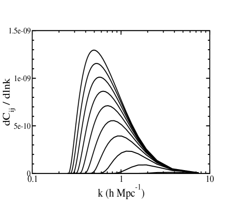
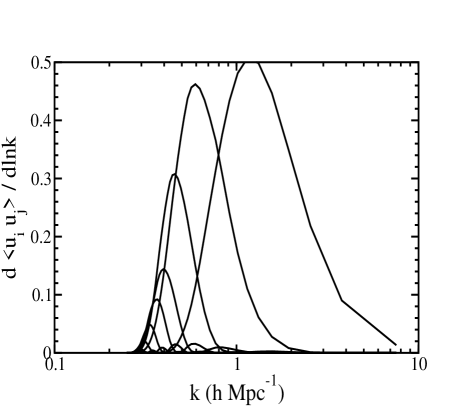
Figure 1: Derivatives $dC_{ij}^{\kappa}/d\ln k$ (left panel) and $d\langle u_{i}u_{j}\rangle/d\ln k$ (right panel) at multipole $\ell=1100$. Here $C_{ij}^{\kappa}$ are the original cross-power spectra and $\langle u_{i}u_{j}\rangle$ are the covariance of the new combinations of shear, defined in Eq. (5). Note the coverage in $k$ for the new eigenmodes; the ones that have most of their weight at high wavenumbers are most sensitive to the parameter $a$. The overall normalization in each panel is arbitrary, but the relative size of the modes is not.

For the bias in the matter power spectrum, our fiducial model is as in Eq. (2) with $a=1.0$ and $f(k)=(k/k_{*})^{\alpha}$. This model phenomenologically describes the baryonic effects if we further set $\alpha\sim 3$ and $k_{*}\sim 10h\,{\rm Mpc}^{-1}$ White_baryon ; LosAlamos and these are the values we use, although we explored a range of other values and found similar results. Finally, to compute the bias in the cosmological parameters due to the small-scale bias, we follow the standard formalism that uses the Fisher matrix described in e.g. Ref. Huterer_Takada .

III 1-point nulling

Let us first consider using $N_{s}$ specific linear combinations of shears in individual redshift bins, specifically $\sum_{j=1}^{N_{s}}Q_{ij}\gamma_{j}(\mbox{\boldmath$\theta$})$, where the coefficients $Q_{ij}$ are independent of the angular position of the galaxy. In other words, each linear combination gives equal weight to all galaxies in the $j$th redshift bin. Our goal is to find specific linear combinations that are most sensitive to the nuisance parameter $a$ and simply throw them out. The nice feature of this problem is that it is tractable analytically.

Let us fix the multipole $\ell$ and define $\tilde{\gamma}_{(\ell,m),i}\equiv a_{(\ell,m)i}$, where $a_{(\ell,m),i}$ is the spherical harmonic coefficient of the shear map in redshift bin $i$. The only things we really need to know about $\tilde{\gamma}_{(\ell,m),i}$ are its mean and variance

$$\langle\tilde{\gamma}_{(\ell,m),i}\rangle=0,\,\,\,\,\,\,\langle\tilde{\gamma}_{(\ell,m),i}\tilde{\gamma}_{(\ell^{\prime},m^{\prime}),j}\rangle=\delta_{\ell\ell^{\prime}}\delta_{mm^{\prime}}C^{\kappa}_{ij}(\ell),$$ (3)

Now consider the linear combinations

$$u_{i}=\sum_{j=1}^{N_{s}}Q_{ij}\tilde{\gamma}_{(\ell,m),j}.$$ (4)

where hereafter we drop the subscript $(\ell,m)$ from $u_{i}$. The covariance matrix of those combinations is

$$\langle u_{i}u_{j}\rangle=\sum_{k,l}Q_{ik}Q_{jl}C_{kl}={\bf q}^{(i)T}\,{\bf C}\,{\bf q}^{(j)}\vspace{-0.3cm}$$ (5)

where the column vector ${\bf q}^{(i)}$ is defined as the i^th row of the matrix ${\bf Q}$, and the matrix ${\bf C}$ has elements $C^{\kappa}_{kl}=\langle\tilde{\gamma}_{(\ell,m),k}\tilde{\gamma}_{(\ell,m),l}\rangle$. Say we only had a measurement of a single $u_{i}\equiv u$. The likelihood for $u$ (in the Fisher matrix approximation) is gaussian

$$\mathcal{L}\propto{1\over\sqrt{R}}\exp{\left({-u^{2}\over 2R}\right)}.$$ (6)

where $\langle u^{2}\rangle\equiv R={\bf q}^{T}\,{\bf C}\,{\bf q}.$ and we suppressed the index $i$ on ${\bf q}$ as well. Then we want to determine the ${\bf q}$ by maximizing the error in $a$, or minimizing (after a bit of algebra)

$$F_{aa}\equiv\left<-{\partial^{2}\over\partial a^{2}}\ln\mathcal{L}\right>={1\over 2R^{2}}\left({\partial R\over\partial a}\right)^{2}.$$ (7)

We now need to solve the following problem: find the column vector ${\bf q}$ that maximizes $F_{aa}$ in Eq. (7), given the $N_{s}\times N_{s}$ covariance matrix ${\bf C}$. Fortunately, this problem is well known and can be solved using standard techniques (e.g. TTH ; Watkins ). The solution is to consider

$$\left({\bf L}^{-1}{\partial{\bf C}\over\partial a}({\bf L}^{-1})^{T}\right)\left(\bf{L}^{T}{\bf q}\right)=\lambda\left(\bf{L}^{T}{\bf q}\right).$$ (8)

where ${\bf L}$ is a lower triangular matrix satisfying ${\bf C}=\bf{LL^{T}}$. Eq. (8) is an eigenvalue-eigenvector relation for ${\bf L}^{T}{\bf q}$ which we can solve to obtain ${\bf q}$. It can easily be shown that the error in $a$ from measurement of any single combination $u_{i}$ is $\sqrt{2}/|\lambda_{i}|$, and that $\langle u_{i}u_{j}\rangle=\delta_{ij}$. Therefore, we get the whole spectrum of uncorrelated combinations of shear ordered by their sensitivity to the small-scale parameter $a$. Again, recall that we need to repeat the same procedure at every multipole $\ell$ (or, multipole bin centered at $\ell$).

We find that the Fisher information on the parameter $a$ is heavily dominated by one (or a few) particular combinations of shears. For example, for the multipole bin centered at $\ell=1100$ and 4-bin tomography, the eigenvalues $\lambda$ are: $7.0\cdot 10^{-6}$, $4.2\cdot 10^{-5}$, $3.3\cdot 10^{-4}$, and $1.3\cdot 10^{-2}$. Clearly, by far the most information about the nuisance parameter $a$ is carried in the eigenvector corresponding to the fourth eigenvalue. This eigenvector is (after adjusting the unimportant overall normalization for clarity) $\tilde{\gamma}_{1}-5.3\tilde{\gamma}_{2}+10.2\tilde{\gamma}_{3}+5.8\tilde{\gamma}_{4}$. Therefore, this combination of shears at $\ell=1100$ is most sensitive to the parameter $a$ and would be the one to drop.

Figure 1 shows $dC_{ij}^{\kappa}/d\ln k$ and $d\langle u_{i}u_{j}\rangle/d\ln k$ at multipole $\ell=1100$, now for a 10-bin tomography, where $C_{ij}^{\kappa}$ are the original cross-power spectra and $\langle u_{i}u_{j}\rangle$ are the covariances of the linear combinations of shears $u_{i}$ defined in Eq. (4). It is clear that the covariances of the $u_{i}$ have a more differentiated wavenumber dependence than the original $C_{ij}^{\kappa}$. However, because of the width of the gravitational lensing kernel, the weights $d\langle u_{i}u_{j}\rangle/d\ln k$, shown in right panel, are still strongly overlapping.

First, consider the fiducial case where we keep all information in the survey, but add a single new parameter $a$ describing the small-scale effect. If the form of the small-scale effect is known exactly, we find that the additional degeneracy introduced by the new parameter $a$ is negligible, and marginalized errors in cosmological parameters increase by only a few percent relative to the case when $a$ is fixed. This is not surprising, as the parameter $a$ enters the observables in a different way than the cosmological parameters, and the fiducial survey is powerful enough to determine them all without substantial loss of accuracy.

Let us now drop the combination $u_{i}$ that is the most sensitive to parameter $a$. We find that the marginalized error on the parameter $a$ increases by several orders of magnitude while increasing the cosmological parameter accuracies only by several tens of percent. While this sounds like fantastic news, we should remember that we optimistically assumed that we were able to exactly guess — and parametrize — the form of the small-scale effect $f(k)$. In reality, we will be able to guess $f(k)$ only approximately, and the difference between the true and guessed $f(k)$ will lead to biases in the measured cosmological parameters. The real figure of merit is the ratio of the bias due to the incorrectly guessed $f(k)$ and the fiducial accuracy in any given cosmological parameter. Clearly, our goal should be to strike balance between the systematic bias and the statistical precision, minimizing the former while not increasing the latter by more than a few tens of percent.

Table 1 shows the errors and biases in $w$ when between zero and two combinations of shear, out of ten total, were dropped, and alternatively, when multipoles $\ell>\ell_{\rm max}$ were dropped. While our 1-point nulling works impressively well, the cut in multipole space is as, and perhaps even more, impressive. For example, to achieve the same statistical error as in 1-point nulling with one combination of shears dropped (error $\gtrsim 100\%$ bigger than the fiducial one) we can alternatively cut all multipoles at $\ell>1000$, but then the bias with cutting in $\ell$ is more than two times smaller than the bias with nulling! We have checked that these results are qualitatively unchanged with a different choice of both the actual and the guessed bias.

IV 2-point nulling

Inspection of Table 1 shows that one problem with 1-point nulling is that it does not have enough resolution in choosing how much of the small-scale structure to null. For example, dropping the single combination of shears that is most sensitive to the parameter $a$ increases the error in $w$ by about 150%, which is too much to tolerate regardless of the success in nulling out the unwanted bias in $P(k,z)$. The lack of ability to perform nulling more gradually is not too surprising, as there are only $N_{s}$ linear combinations to choose from.

Ideally we would like to have a better resolution in the eigenvalues $\lambda_{i}$ and thus obtain a better leverage in controlling the cosmological parameter degradations as a function of the nulling efficiency. One way to remedy that is to form linear combinations of the convergence power spectra $C_{ij}^{\kappa}$, as there are $N\equiv N_{s}(N_{s}+1)/2$ of them

$$v_{i}\equiv\sum_{j=1}^{N}\tilde{Q}_{ij}C_{j}^{\kappa}(\ell)$$ (9)

where $\tilde{Q}_{ij}$ are coefficients (different from $Q_{ij}$ in the previous section) and we denote a pair of redshift bins by a single subscript; here $i$ and $j$ take values from $1$ to $N$. The goal is to find the linear combination(s) $v_{i}$ that produce the largest Fisher matrix element $F_{aa}$. While the 1-point procedure can be repeated, the optimization problem, sadly, cannot be solved analytically as before because $\langle C_{j}^{\kappa}\rangle\neq 0$, and we needed that assumption for the expression for $F_{aa}$, Eq. (7), to take its simple form. Therefore, we choose to find the optimal combinations of the convergence power spectra by brute force. Using Powell’s minimization method NR , we find the linear combination $v_{1}$ that has maximal $F_{aa}$. Using the Gram-Schmidt algorithm, we then project to the $(N-1)$ dimensional subspace, perform the maximization again, and find the second most sensitive combination, $v_{2}$. And so on, until we find all combinations of the power spectra ordered by their sensitivity to the small-scale effect. As with the 1-point function, we apply this algorithm at every $\ell$ separately, where $\ell$ is the center of the corresponding band power window in multipole space.

1-point Nulling			Cutting above $\ell_{\rm max}$
Skipped	$\sigma(w)$	$\delta(w)$	$\ell_{\rm max}$	$\sigma(w)$	$\delta(w)$
0	0.054	0.085	10000	0.054	2.630
1	0.130	0.023	3000	0.073	0.101
2	0.291	0.003	1000	0.117	0.010

Table 1: Nulling out shear combinations that are most sensitive to $a$ vs. simply cutting measurements at some $\ell_{\rm max}$ for a 10-bin tomography case. The nulled $\delta P(k)$ was assumed to go as $k^{3}$ (with $k_{*}=10$h Mpc^-1), the actual one as $k^{3.5}$. While nulling in principle works well, it leads to degradation in statistical errors that are about 150% or larger, and therefore too large to tolerate. On the other hand, simply throwing out power beyond some $\ell_{\rm max}$ is surprisingly efficient; for example, restricting to $\ell_{\rm max}=1000$ leads also to a similar $\gtrsim 100\%$ increase in $\sigma(w)$, but with the bias in $w$ that is smaller than with 1-point nulling. More importantly, cutting in $\ell$ can be done gradually, while the 1-point nulling necessarily leads to jumpy changes in the statistical error and bias.

We indeed find that the resolution in nulling is greater with 2-pt nulling than with 1-point; for example, throwing out the most sensitive combination increases $\sigma(w)$ by about 40%, and not 150%. However, we found two problems with 2-point nulling. First, as before we find that simple cutting in $\ell$ works about as well or better. In addition, we find that the biases in cosmological parameters are substantially suppressed only if the form of the bias is nearly precisely known, and not in more realistic situations when the bias is guessed incorrectly. These conclusions are unchanged even after trying different forms of $f(k)$, looking at different cosmological parameters, different values of $k_{*}$, and different numbers of survey redshift bins. Therefore, unless our 2-point procedure is substantially improved in some way, 1-point nulling is the more effective approach.

V Cutting in wavenumber $k$

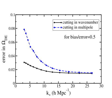
Figure 2: Comparison of the cutting in wavenumber $k$ vs. the cutting in multipole $\ell$. Left panel: evolution of error vs. the (absolute) bias in $\Omega_{\rm DE}$ with increased aggressiveness in cutting in $k$-space (solid black curve) or $\ell$-space (dashed blue curve). The cut is increasingly more severe going from bottom right to top left. Here we use a 4-bin tomography case with the small-scale effects going as $(k/k_{*})^{3}$ with with $k_{*}=10h\,{\rm Mpc}^{-1}$. For orientation, we show one value each of $\ell_{\rm max}$ and $k_{\rm cut}$ on the curves along which they vary; these are roughly the points where the bias is reduced to a fraction ($\sim 0.5$) of the statistical error, and in this case the total error with the $k$-cut is about 50% smaller than that with the $\ell$-cut. Right panel: statistical error in $\Omega_{\rm DE}$ after cutting as a function of the scale at which the small-scale bias enters, $k_{*}$, for the $k$ and $\ell$ cutting. With each method and for each value of $k_{*}$, just enough cutting is performed so that the remaining bias in $\Omega_{\rm DE}$ is equal to one half of its statistical error. Note that the two methods are comparable if the bias enters at small scales (high $k_{*}$), but if the bias affects much larger scales the $k$-cutting is clearly more effective as it leads to a smaller final error in $\Omega_{\rm DE}$.

Another simple strategy is to simply throw out contributions to the band powers coming from wavenumbers greater than some (comoving) cutoff $k_{\rm cut}$. Assume that the Limber’s approximation integral over the large-scale structures is discretized, with $N_{p}$ (rather than infinitely many) lens planes. Then, assigning a single subscript $i$ for any of the $N$ cross-power spectra, we have

$$C_{i}^{\kappa}(\ell)=\sum_{j=1}^{N_{p}}W_{ij}P(k_{j},z_{j})$$ (10)

where $W$ are suitably defined weights that depend on the lensing geometry and the distribution of galaxies and $P(k_{j},z_{j})$ is the matter power spectrum evaluated at some wavenumber $k_{j}=\ell/r(z_{j})$ and redshift $z_{j}$ of the lens plane in question. We now form a $N\times N_{p}$ matrix with the $(i,j)$ entry equal to $W_{ij}P(k_{j},z_{j})$; we have $N=10$ (corresponding to $N_{s}=4$ redshift bins) and $N_{p}=59$. Then we simply transform this matrix to the lower triangular form. The rows now represent linear combinations of the convergence power spectra, and new matrix entries are their weights. Of course, all $N$ rows still contain the same information as before, as we simply performed a linear operation on the $C^{\kappa}$s. However, by considering the first $M$ rows only ($M<N$), we can avoid using any information coming from wavenumbers greater than the wavenumber on $(N_{p}-M)$th lens plane. As before, we repeat the procedure at each multipole band centered at $\ell$. For simplicity we hold $k_{\rm cut}$ independent of $\ell$, and then higher $\ell$ implies higher $k_{j}$ for a fixed lens plane — therefore, more combinations will be cut at higher $\ell$, until some multipole $\ell\simeq k_{\rm cut}r(z_{\rm max})$ where no information at $k>k_{\rm cut}$ will be left. Note too that, unlike the 1 and 2-point nulling, cutting in $k$ does not require a guess of the offending small-scale effect as all information beyond $k_{\rm cut}$, “good” and “bad”, is thrown out.

To explore the efficacy of this type of nulling, we perform it for a variety of values $k_{\rm cut}$, then compare to the “gold standard” of dropping multipole power spectra above a fixed $\ell_{\rm max}$. Overall, we find that cutting in $k$ works better than cutting in $\ell$, as expected since our small-scale contamination is defined in $k$. However, the two methods are essentially equally powerful unless the small-scale effect enters at very large scales (i.e. if $k_{*}$ is small), and in that case the $k$-cut can be significantly more powerful; see Fig. 2. This is easy to understand as, from the relation $k\simeq\ell/r(z)$, we see that even if stringent cutting in $\ell$ is performed, some amount of high $k$ modes, corresponding to low redshift structures, will be left in the data — and these high $k$ modes can be extremely damaging if $k_{*}$ is small since the bias in the observables goes as a power law in $k/k_{*}$. It is also interesting to note that cutting in $k$ is equivalent to removing the low-redshift structures from the data — in other words, instead of cutting above some $k_{\rm cut}$, one could equivalently choose not to use lens galaxies with (photometric) redshifts less than $z_{\rm cut}$ where $r(z_{\rm cut})=\ell/k_{\rm cut}$. Which of these two possibilities is more feasible in practice is an interesting question, but outside the scope of this work.

Current estimates indicate that the effective scale of various small-scale effects is anywhere from a few to a few tens of $h\,{\rm Mpc}^{-1}$ (e.g. White_baryon ; LosAlamos ; Zhan_Knox ). If $k_{*}$ is closer to the lower end of this range for any of these effects, cutting out the high wavenumbers (or low-redshift structures) may prove extremely beneficial.

VI Discussion and Conclusions

We have described and explored three different strategies for nulling out small-scale information in weak lensing power spectrum measurements, with the idea of protecting against uncertain, approximately known contamination while preserving most of the sensitivity to cosmological parameters.

The 1-point nulling tomography uses select linear combinations of shear in different redshift bins so as to maximally reduce the survey’s sensitivity to small-scale bias. The algorithm for achieving this is well known and largely analytic, and it produces the desired linear combinations ordered by how sensitive they are to the parameter $a$ describing the small-scale bias. Figure 1 shows that, as expected, the combination that is most sensitive to the small-scale bias has weight at smaller scales than the other combinations. Since in a realistic situation we will only have approximate understanding of the true bias, we test the performance of 1-point nulling by assuming the fiducial bias is a power law in wavenumber, while the fit bias, normalized by the parameter $a$, is a different power law. We find that even as just one linear combination of shear is dropped from the analysis (the one most sensitive to the parameter $a$) the biases in cosmological parameters are sharply reduced. However, in that case the increase in cosmological parameter errors is about 150%. Whether that is too large to tolerate depends on the fiducial power of the survey and on the deleterious effect of other, unrelated systematic errors.

The problem of large initial degradation can in principle be ameliorated by 2-point nulling, where we form linear combinations of the cross power spectra (rather than shear). Because the number of cross power spectra is of order the number of redshift bins squared, we have many more observables at our disposal and can achieve a finer resolution in the amount of nulling performed, and hence in cosmological parameter error degradation. Unfortunately 2-point nulling does not have a nice analytic solution and linear combinations of power spectra that are most sensitive to the small-scale bias need to be found by brute force. We find that the method works well in cases when the functional form of the bias can be guessed accurately. If the exact form for the bias is guessed incorrectly, however, 2-point nulling produces biases in cosmological parameters that do not decrease as the most sensitive combinations are dropped. We conclude that 1-point nulling is more effective than the 2-point approach, and this is unlikely to change unless a substantial improvement to our 2-point procedure is found in the future.

While both 1 and 2-point nulling are effective, we found that they are not significantly better than the simplest strategy of dropping the highest multipoles of the convergence power spectra. [This may not be too surprising in retrospect: decreasing $\ell_{\rm max}$ from 10000 to 3000, for example, increases the cosmological parameter error bars by only $\sim 30\%$ while having a tremendous impact in removing a variety of small-scale contaminations — in other words, the price to pay with dropping the highest multipoles is relatively small, and this procedure is already reasonably effective.] This motivated us to explore yet another, but very different, method for removing the small-scale biases. We proposed a method of removing all information above some wavenumber $k_{\rm cut}$ or, roughly equivalently, removing structures below some redshift from the data. This approach is different from the previous two in that the functional form of the bias need not be known, and all information above $k_{\rm cut}$, useful or not, is thrown out. This works the best of all methods, leading to cosmological parameter errors that are 10-50% percent smaller than those with the $\ell$ space cut, and by up to a factor of two if the small-scale effect enters at sufficiently large scales. Given that weak lensing shear data is likely to be biased by large nearby structures (e.g. a large cluster of galaxies at low redshift), some form of cutting in wavenumber will surely be beneficial to protect against biases.

All of the aforementioned techniques require rough knowledge of the cosmological model so that the fiducial convergence power spectra (i.e. those not including the small-scale bias) are known to a good accuracy, and can be manipulated to null out the unwanted effects. This should not be a problem in the future, as the cosmological parameters are already reasonably well determined with the combination of cosmic microwave background, type Ia supernovae and large-scale structure constraints. However, systematic errors in weak lensing measurements are a bigger concern. While the study in this paper was precisely concerned with removing biases due to a class of systematics – uncertain theoretical predictions on small scales – there will be other systematics in weak lensing measurements that can roughly be divided into redshift errors and additive and multiplicative errors in measurements of shear wlsys . Those errors are likely to depend on numerous factors (e.g. observational season, galaxy morphology, etc.) and are uncertain at this time. We do not believe that the systematics will significantly affect the nulling techniques described in this paper since the systematics, provided they are small, should be a lower-order contribution to our observables (which are linear or quadratic in shear). Nevertheless, just as with all other applications of weak lensing in the next generation experiments, incorporating the systematics into the nulling tomography will be an important and challenging task.

In conclusion, we strongly believe that the strategies that we described will find application in weak lensing data mining. We only considered the convergence power spectrum information here. Other aspects of weak lensing, such as mapping of dark matter, depend more critically on the small-scale information, and it might be that nulling-type techniques will reach their full potential in precisely those applications. It is likely that these interesting possibilities will be considered in the future.

References

- (1) Hu, W. 1999, ApJ, 522, L21
- (2) Hui, L. 1999, ApJ, 519, L9
- (3) Huterer, D., 2002, Phys. Rev. D, 65, 063001
- (4) Hu, W. 2003, Phys. Rev. D, 66, 083515
- (5) Refregier, A. et al. 2003, MNRAS, 346, 573
- (6) Abazajian, K. & Dodelson, S. 2003, Phys. Rev. Lett., 91, 041301
- (7) Song, Y.-S. & Knox L. 2004, Phys. Rev. D, 70, 063510
- (8) Takada, M. & Jain, B. 2004, MNRAS, 348, 897
- (9) Ishak, M., Hirata, C.M., McDonald, P. & Seljak, U. 2004, Phys. Rev. D, 69, 083514
- (10) Vale, C. & White, M. 2003, ApJ, 592, 699
- (11) White, M. & Vale, C. 2004, Astropart. Phys., 22, 19
- (12) Heitmann, K., Ricker, P. M., Warren, M. S., Habib, S., 2004, astro-ph/0411795
- (13) Huterer, D. & Takada, M. 2005, Astropart. Phys., 23, 369
- (14) White, M. 2004, Astropart. Phys., 22, 211
- (15) Zhan, H. & Knox, L. 2005, ApJ, 616, L75
- (16) Takada, M. & White, M. 2004, ApJ, 601, L1
- (17) Aldering, G. et al. 2004, PASP, submitted (astro-ph/0405232)
- (18) Tegmark, M., Taylor, A. N., & Heavens, A. F. 1997, ApJ, 480, 22
- (19) Watkins, R., Feldman, H. A., Chambers, S. W., Gorman, P. & Melott, A. L. 2002, ApJ, 564, 534
- (20) Press, W. H., Flannery, B. P., Teukolsky, S.A., and Vetterling, W.T. 1992, Numerical Recipes in C, Section 10.5, Cambridge University Press.
- (21) Huterer, D., Takada, M., Bernstein, G. & Jain, B. 2005, astro-ph/0506030