T Tauri stellar magnetic fields: He i measurements

Abstract

We present measurements of the longitudinal magnetic field in the circumstellar environment of seven classical T Tauri stars. The measurements are based on high-resolution circular spectropolarimetry of the He i $\lambda 5876$ emission line, which is thought to form in accretion streams controlled by a stellar magnetosphere. We detect magnetic fields in BP Tau, DF Tau and DN Tau, and detect statistically significant fields in GM Aur and RW Aur A at one epoch but not at others. We detect no field for DG Tau and GG Tau, with the caveat that these objects were observed at one epoch only. Our measurements for BP Tau and DF Tau are consistent, both in terms of sign and magnitude, with previous studies, suggesting that the characteristics of T Tauri magnetospheres are persistent over several years. We observed the magnetic field of BP Tau to decline monotonically over three nights, and have detected a peak field of 4 kG in this object, the highest magnetic field yet observed in a T Tauri star. We combine our observations with results from the literature in order to perform a statistical analysis of the magnetospheric fields in BP Tau and DF Tau. Assuming a dipolar field, we determine a polar field of $\sim 3$ kG and a dipole offset of 40° for BP Tau, while DF Tau’s field is consistent with a polar field of $\sim-4.5$ kG and a dipole offset of 10°. We conclude that many classical T Tauri stars have circumstellar magnetic fields that are both strong enough and sufficiently globally-ordered to sustain large-scale magnetospheric accretion flows.

1 Introduction

It has been postulated that accretion in low-mass pre-main-sequence stars is magnetically-controlled (e.g. Köenigl, 1991; Collier Cameron & Campbell, 1993), with the magnetic field disrupting a Keplerian disc and the accreting material plummeting along the field lines onto the stellar surface. This model provides an attractive solution to the angular momentum dissipation that is required to produce a slowly rotating protostar, and synthetic emission line profiles produced assuming a magnetospheric accretion via a dipolar field are able to reproduce some characteristics of the observed profiles (e.g. Hartmann et al., 1994; Muzerolle et al., 1998).

One of the key requirements of this model is the presence of a strong, relatively structured, magnetic field a few stellar radii above the star. Traditional methods for measuring surface magnetic fields rely on the Zeeman effect. Actual splitting of absorption line profiles is rarely observed, because other broadening mechanisms (rotation, pressure, turbulence etc) usually dominate over the relatively weak Zeeman effect. Nonetheless, if the intrinsic shape of the profile is well understood, it is possible to attribute the residual broadening to Zeeman splitting, and hence measure a magnetic field strength. This method has been used with some success on classical T Tauri stars (CTTSs), and surface fields of a few kilogauss have been determined (Basri et al. 1992; Guenther et al. 1999; Johns-Krull et al. 1999).

Although surface magnetic fields have been measured for a few CTTSs, it is not clear how the strength of these fields changes with radius and how ordered they are (e.g. Safier 1998). Measurements of circumstellar magnetic fields require observations of the Zeeman effect in an emission line, and here the Zeeman broadening technique fails – primarily because the lines are broadened by the bulk motion of the accreting gas, and the intrinsic profile of the line cannot be determined with any certainty. Fortunately Zeeman splitting also results in a polarization signature, with the $\sigma$-components of the transition being circularly polarized in opposite senses. The separation between these components is directly proportional to the mean longitudinal field strength (Babcock, 1947).

Johnstone & Penston (1986, hereafter JP) attempted to measure the magnetic fields in three T Tauri stars using this effect, and found a 2.3-$\sigma$ detection ($-548$G) for RU Lup, which was not confirmed by later observations (Johnstone & Penston, 1987). More recently Johns-Krull et al. (1999) measured the Zeeman shift in circular polarization of the He i $\lambda 5876$ in BP Tau, using an echelle spectrograph on a 2.7-m telescope at McDonald Observatory. The He i $\lambda 5876$ line is thought to form above hot impact regions on the stellar surface in streams of gas being accreted by the star (e.g. Valenti et al. 1993). Edwards et al. (1994) found that the line showed an inverse P Cygni profile for stars with high levels of continuum veiling – two well-known accretion indicators. Johns-Krull et al. (1999) inferred a mean longitudinal magnetic field of 2.4 kG, which was the first direct evidence of magnetic accretion in a CTTS. Similar observations on three more CTTSs were presented by Johns-Krull et al. (2001) and Valenti et al. (2003).

Here we present measurements of the longitudinal magnetic field in seven CTTSs using the He i $\lambda 5876$ emission line. The aim of these observations was to expand the sample of CTTSs with known fields and to examine the long-term (many rotation cycles) stability of the magnetosphere.

2 Observations and data reduction

2.1 Zeeman effect

In this paper we exploit the Zeeman effect to measure the magnetic field around CTTSs. If there is a net magnetic field along the observer’s line of sight, a spectral line is split and the separation in wavelength between the two $\sigma$-components is a measure of the field strength. The wavelength shift is

$$\Delta\lambda=2\,\frac{e}{4\pi m_{e}c^{2}}\,\lambda^{2}\,g_{\mathrm{eff}}\,B_{z}$$ (1)

$$\phantom{\Delta\lambda}=9.34\times 10^{-7}\,\lambda^{2}g_{\mathrm{eff}}\,B_{z}\,\textrm{m\AA}\,\textrm{kG}^{-1}$$ (2)

where $\lambda$ is the rest wavelength of line (in Å), $g_{\mathrm{eff}}$ is the effective Landé $g$-factor of the line transition and $B_{z}$ is the net longitudinal magnetic field (Mathys, 1991). The value of $g_{\mathrm{eff}}$ adopted for He i $\lambda 5876$ was $1.11$, but the line is formed by multiple transitions and $g_{\mathrm{eff}}$ is dependent on the environment (see e.g. Johns-Krull et al. 1999). For other spectral lines, Landé $g$-factors were obtained from the solar line list table of J.F. Donati reproduced at http://bass2000.bagn.obs-mip.fr.

2.2 Observations

Spectra were obtained with the ISIS spectrograph at the Cassegrain focus of the 4.2-m William Herschel Telescope. The configuration for circular spectropolarimetry is described in Tinbergen & Rutten (1992). A quarterwave plate first converts from circular to linear polarization. Light from the target object then passes through one aperture of a comb dekker; the other apertures sample the background sky emission. A comb dekker with 20-arcsec apertures was used for all exposures except the tungsten lamp flat-fields. The star and sky beams all pass through a Savart plate which spatially separates the orthogonal linear polarizations into o- and e-beams, each of which then passes through the standard spectrograph optics and is recorded on a CCD detector. Rotating the quarterwave plate between exposures, by $90\degr$ relative to the first position, swaps the polarization sense of each beam and should reverse direction of the measured wavelength shift. Many of the possible systematic errors in the optics or detector would lead to unequal inferred magnetic field magnitudes from a pair of exposures, and this is the first of several tests we can use to assess the veracity of our results.

The observations were made on nights beginning 2001 December 3–5 and 2002 December 21–23 with the R1200 grating on the ISIS red arm. Approximately half of each run was lost to weather or technical problems. We observed calibration targets, and seven bright CTTSs in the Taurus-Auriga region with known He i emission lines (Edwards et al., 1994). The TEK4 CCD detector was used during the 2001 run, providing $0.40\rm{\AA}$ per pixel reciprocal dispersion; the newer MARCONI2 CCD was employed in 2002 to obtain $0.22\rm{\AA}$ per pixel. The resolution achieved was 0.7Å (FWHM of the arc lines). Maximum sensitivity of the system was selected by inserting a circular-polarizing filter during setup, and finding the quarterwave-plate angle that gave the maximum contrast between the intensity of the o- and e-beams. Observations of the target objects (typically 1000-s per frame) were bracketed by exposures with copper-neon and copper-argon comparison lamps to provide a wavelength calibration.

2.3 Data reduction

The procedure for obtaining a magnetic field measurement requires cross-correlation of two spectra recorded simultaneously on different areas of the CCD. Differential errors in the extraction or calibration of the spectra will create a false magnetic field detection; it is important to test the systematic effects are well below the (less than one pixel) expected Zeeman wavelength shift.

Each CCD frame was first bias-subtracted and flat-fielded. The flat-field frames had a large intensity gradient towards the edges where vignetting was significant, so these frames were normalised so that they had a value close to 1 across the central area, where the spectral lines of interest were recorded. In the 2002 run, flat-field frames were recorded at both quarterwave-plate rotation positions ($\theta_{0}$, $\theta_{0}+90\degr$) and the appropriate master flat-field used for correcting each of the target exposures in a pair. Similarly, the arc comparison frames were recorded at both quarterwave-plate angles, and the appropriate arc spectrum was used for calibrating each target spectra.

The 2001 observations contained calibration frames made at only one rotation angle of the quarter-wave plate, and it was necessary to test the effect of reducing data from both quarter-wave plate positions with a flat-field from just one position. Test reductions were carried out with the 2002 data using mismatching flat-fields and the derived wavelength shifts were not significantly different from the results using flat-fields from both quarter-wave plate positions. These results were also unaffected when a single arc-lamp exposure was used to calibrate each complementary pair of target exposures, so we had confidence in using these techniques for the 2001 data.

For each exposure, the two stellar spectra (corresponding to the left- and right-handed polarisation states) were extracted, as well as two spectra sampling the sky background. The sky spectra were of very much lower intensity than the stellar continuum and were unstructured over the wavelength extent of the He i $\lambda 5876$ line. Tests on sample frames showed that sky subtraction did not affect the results; it was decided that this process only contributed noise and should be omitted from the data reduction sequence.

Spectra of the arc lamps were obtained from their frames using the same extraction windows used for the stellar spectra, then a third-order polynomial wavelength scale was fitted using identifiable emission lines as references. The typical RMS error from the fit to the arc lines was $\sim 0.03$Å. The four stellar spectra (an o- and an e-beam recorded at each quarterwave plate position) were rebinned to a common linear wavelength scale in preparation for determining the wavelength shift. The scale was chosen to be similar to that of the individual spectra.

2.4 Cross-correlation analysis

A range of wavelength bins containing the emission or absorption line of interest were copied from the full spectra for cross-correlation using the procedure described in JP. We manually inspected the spectra to choose the limits for the line region, rather than employ an automated procedure. The emission lines in the T Tauri-class spectra were generally strong compared to the continuum, so most of the photons were recorded in a narrow wavelength range and it was not felt necessary to include the line wings where it was difficult to identify the transition to the local continuum intensity.

The two rebinned spectra from each CCD frame were cross-correlated by evaluating a $\chi^{2}$ statistic, S, for one spectrum being used as a model for the other (after allowing for intensity rescaling). As described in JP, we made whole-pixel shifts between the spectra and fitted a parabola to the three values of S that were closest to the minimum value, S(min). The minimum turning point of the parabola gives the wavelength shift between the two spectra, $\Delta\lambda$, that is used to obtain the magnetic field strength $B_{z}$ (Equation 2). Table 1 lists $B_{z}$ for each of the target exposures.

Although we had propagated uncertainty estimates for each pixel or wavelength bin throughout the data reduction, when the spectra were rebinned to a common wavelength scale it became non-trivial to estimate the uncertainty contribution from each source bin to each target bin because the errors are then correlated. We therefore used the ratio of variances method (described in JP; Lampton et al. 1976) to estimate the 1-$\sigma$ uncertainty interval for each Zeeman wavelength shift. The interval is found from the cross-correlation shift $\chi^{2}$ statistic, S, relative to S(min), its value at the minimum turning point of the parabola, such that:

$$\mathrm{S}<\mathrm{S(min)}\left[1+\frac{\mathrm{p}}{\mathrm{N}^{\prime}-\mathrm{p}}F(\mathrm{p},\,\mathrm{N}^{\prime}-\mathrm{p},\,\alpha)\right]$$ (3)

where $\mathrm{p}$ is the number of free parameters used to find S(min); $\mathrm{N}^{\prime}$ is the number of independent wavelength bins in the spectra; $\alpha$ is the confidence level required (i.e. $\sim 0.68$ for the 1-$\sigma$ interval); and $F(\mathrm{p},\,\mathrm{N}^{\prime}-\mathrm{p},\,\alpha)$ is the Fischer-Snedecor ratio of variances function. One spectrum from each pair was scaled in intensity to match the other, and then shifted in wavelength, so $\mathrm{p}=2$. We follow the advice of JP, who show that after rebinning the spectra, the effective number of independent wavelength bins is reduced to $5/6$ of the number of bins in the raw spectra. The interval in Equation 3 defines a range of wavelength shifts that gives (with Equation 2) the 1-$\sigma$ uncertainties on the $B_{z}$ values presented in Table 1.

A hybrid scheme was also tried which used inverse variance weighting when calculating the $\chi^{2}$ statistics. The advantage of this alternative was that the variance associated with each wavelength bin included information about the flat-field uncertainties, detector noise etc. The results were not significantly altered by this change in procedure, and we concluded that the original cross-correlation method was adequate.

We found that small changes made to our procedures (such as altering the wavelength limits of the emission line, or the trials using single calibration frames in Section 2.3) typically perturbed the individual measurements by approximately $100$G. When the uncertainties in the polarization standards (Section 2.5) are also taken into account, we estimate that the systematic errors in our results are probably of magnitude $\sim 200$G and we would not confidently claim to detect magnetic fields of lesser strength. We have not attempted to account for the systematic effects when quoting uncertainty intervals in this paper; they are always the formal errors derived from the cross-correlation procedure.

The magnetic field of a target T Tauri star was expected to vary little over the duration of the observations (less than $\sim 1$h) on a given night. We therefore obtained a nightly $B_{z}$ measurement for each star by computing a mean value weighted by the inverse variance of the individual estimates. Fig.1 shows both the individual measurements and the mean values, with their 1-$\sigma$ uncertainty intervals. We present the combined results in Table 2, along with characteristic stellar data from the literature.

Figure 1: Plots of the $B_{z}$ (G) results from individual exposures. The circles are the measurements derived from individual exposures; the horizontal lines are the 1-$\sigma$ uncertainty intervals for those values. Each night’s data for each object were combined using an inverse-variance weighted mean. The vertical solid and dashed lines show the mean and 1-$\sigma$ intervals respectively.

To test our estimates of the 1-sigma uncertanties we can calculate a reduced chi-squared statistic for all our measurements, with respect to the mean for the object on the night in question. This yields a $\chi_{\nu}^{2}$ of 0.836 with 59 degrees of freedom. Since we expect 81 per cent of such experiments to exceed this value, it suggests that both our assumption that the polarization is unchanging within the $\sim$1h of our observations, and our calculation of the uncertainties is broadly correct. Table 2 also gives the values of $\chi_{\nu}^{2}$ for each object on each night. Although there are a couple of uncomfortably high values of $\chi_{\nu}^{2}$ for individual objects on individual nights, given the above result, and the low number of degrees of freedom for the nightly chi-squareds, their statistical significance is unclear. Furthermore, the highest value corresponds to the data with the smallest uncertainty (86G) and thus we would expect it to be affected by the systematic uncertainties that we estimate to be about 200G. We therefore conclude that the $\chi^{2}$ analysis supports our conclusion that there are systematic effects at the 200G level, but above this level our uncertainties are probably correct.

2.5 Test stars

We observed three targets with dependable levels of circular polarization to test our instrumental setup and data reduction process. The Sun has a magnetic field strength much smaller than the sensitivity of our equipment, so it was used as a null reference. Sunlight reflected from Vesta provided practical access to the solar spectrum; for the purposes of this experiment, the asteroid can be considered to be a passive reflector of circularly-polarized light. In poor seeing conditions, only two measurements had reasonable signal-to-noise ratios and these two useful exposures were obtained with the quarterwave plate at the same angle, so we can not test that the same magnitude of wavelength shift is measured as the beams are reversed (as described in Section 2.3). An inverse-variance weighted mean of the shift in the Na i 5889Å line represented a mean field strength $\mathrm{B}_{z}=-20\pm 180$G, which is consistent with the expected null result.

Observations of the magnetic Ap star 53 Cam permitted comparison with measurements published by other authors. Data obtained in both the 2001 and 2002 runs were phased using the ephemeris of Hill et al. (1998). Our two measurements are shown in Fig. 2, along with those from two other sources. Rather than choose a sign convention for $B_{z}$ based on the spectrograph setup, we have assumed that our 53 Cam measurements are consistent with the previously published data, and should therefore both have a positive sign. Our data then are of the magnitude expected from the previous studies, indicating that our measurement technique is reliable. The sign convention adopted is later shown to also be consistent with previous measurements of T Tauri magnetic fields published by other authors.

Figure 2: Magnetic field measurements of the Ap star 53 Cam. Our data are shown as filled squares, along with those of Hill et al. (1998) (open squares) and Wade et al. (2000) (open circles).

Observations were made of a linear polarization standard star to determine whether our instrumentation would apparently detect a Zeeman wavelength shift because of unwanted conversion from linear and circular polarization in the optics. The star HD25443 (5.1 per cent V band linear polarization; Turnshek et al. 1990) was observed during the 2001 run and several spectral lines were cross-correlated. The wavelength shift found by our data reduction process would be equivalent to a magnetic field of $-194\pm 45$G, which would be a significant detection. It is possible that this star does have an intrinsic longitudinal magnetic field, but it is more likely that the apparent wavelength shift between the two beams is caused by imperfect polarization optics. We expect that any effects of polarization cross-talk are going to be within the 200G systematic error estimate we discussed above and do not threaten the validity of our experimental results.

Table 1: Summary of T Tauri star observations and individual results. Times quoted are UT at exposure midpoint. Quarterwave plate rotation angles ($\phi$) are quoted in degrees, relative to the adopted zero point (Section 2.2). Uncertainties in the longitudinal magnetic field, $B_{z}$, are the 1-$\sigma$ interval.

Name	Night	JD$-$2452000	$\phi$	$\Delta\lambda$ (mÅ)	$B_{z}$(G)	$\pm$ 1-$\sigma$		Name	Night	JD$-$2452000	$\phi$	$\Delta\lambda$ (mÅ)	$B_{z}$(G)	$\pm$ 1-$\sigma$
BP Tau	2001 Dec 03	247.476	0	64	1800	1100		DN Tau	2002 Dec 23	632.317	90	53	1490	410
		247.488	90	23	630	340				632.329	0	$-0.4$	$-10$	440
		247.500	0	70	1950	750				632.341	90	21	600	420
		247.512	90	$-16$	$-450$	760				632.353	0	10	270	440
		247.525	0	54	1520	750				632.369	90	42	1160	380
		247.537	90	50	1410	622				632.381	0	15	430	350
	2002 Dec 21	630.385	0	160	4400	1200		GG Tau	2002 Dec 23	632.401	0	$-18$	$-500$	640
		630.391	90	130	3700	1100				632.412	90	33	920	660
		630.412	0	120	3400	1200				632.424	90	0.4	10	500
		630.424	90	150	4100	1200				632.436	0	$-11$	$-320$	560
		630.441	0	130	3500	1100				632.450	90	12	330	520
		630.453	90	140	3900	1300		GM Aur	2002 Dec 22	631.688	90	$-100$	$-2800$	1600
	2002 Dec 22	631.633	90	90	2510	870				631.700	0	$-52$	$-1460$	780
		631.645	0	81	2250	540				631.712	0	$-59$	$-1650$	910
		631.657	0	60	1670	460				631.724	90	6	170	980
		631.668	90	68	1910	620				631.737	90	$-54$	$-1500$	1600
	2002 Dec 23	632.564	0	45	1270	290			2002 Dec 23	632.726	0	$-25$	$-700$	1700
		632.575	90	32	880	660				632.738	90	27	760	501
		632.587	0	41	1140	380				632.747	90	50	1400	1100
		632.599	90	42	1180	680				632.753	0	$-86$	$-2400$	1400
		632.612	0	39	1100	260		RW Aur A	2001 Dec 05	249.700	0	8	210	370
		632.624	90	47	1300	530				249.711	90	22	620	380
DF Tau	2002 Dec 21	630.474	0	$-38$	$-1050$	430				249.723	0	15	410	500
		630.491	90	$-36$	$-1010$	300				249.735	90	22	620	420
		630.506	0	$-28$	$-770$	400			2002 Dec 21	630.659	0	21	600	1700
		630.520	90	$-31$	$-870$	480				630.671	90	29	800	1600
		630.532	0	$-35$	$-970$	530				630.683	0	$-29$	$-800$	1700
		630.544	90	$-41$	$-1150$	360			2002 Dec 23	632.484	90	28	780	880
	2002 Dec 23	632.649	90	$-23$	$-640$	190				632.497	0	3	80	570
		632.661	0	$-38$	$-1060$	280				632.509	90	$-6$	$-160$	830
		632.672	0	$-42$	$-1160$	260				632.521	0	$-5$	$-130$	870
		632.684	90	$-18$	$-490$	170				632.533	90	36	1000	1200
		632.696	90	$-17$	$-480$	170				632.545	0	4	110	820
		632.708	0	$-46$	$-1280$	290
DG Tau	2002 Dec 21	630.564	0	$-18$	$-500$	1500
		630.576	90	25	700	1700
		630.588	0	32	880	1100
		630.600	90	22	620	1100
		630.615	0	$-6$	$-170$	1500
		630.627	90	9	240	2300

3 Results

Here we describe our measurements of individual objects, and review the observational evidence for magnetically controlled phenomena.

3.1 Null detections

Two of the target CTTSs had results that were consistent with zero longitudinal field. Our cross-correlation analysis (Section 2.4) leads to formal 2-$\sigma$ upper limits of $|B_{z}|<0.80$ kG for DG Tau and $|B_{z}|<0.32$ kG for GG Tau. Each of these stars was observed on only one night, so it is possible that the measurements were made at epochs when the orientations of the magnetic fields were unfavourable.

3.2 Possible detections

Table 2: Nightly $B_{z}$ results for each star. The $v\,\sin i$ data are from Hartmann & Stauffer (1989). Other properties for each object were from references: 1. Cohen & Kuhi (1979); 2. Gullbring et al. (1998); 3. Hartigan et al. (1995); 4. Valenti et al. (1993). Mass accretion rate ($\dot{{\rm M}}$) is in units of $10^{-7}\mbox{$\rm{M}_{\odot}\,\mathrm{yr}^{-1}$}$, $\mathrm{v}\,\sin i$ in  $\mbox{km}\,\mbox{s}^{-1}$.

Name	Sp. Type (ref.)	$\mathrm{v}\,\sin i$	$\dot{{\rm M}}$ (ref.)	Night beg.	# Obs.	$B_{z}$(G)	$\pm$ 1-$\sigma$	$\chi^{2}_{\nu}$
BP Tau	K7 (1)	10.0	0.288 (2)	2001 Dec 03	6	920	240	1.57
				2002 Dec 21	6	3820	480	0.106
				2002 Dec 22	4	1980	290	0.361
				2002 Dec 23	6	1170	150	0.093
DF Tau	M0.5 (1)	16	1.767 (2)	2002 Dec 21	6	$-980$	160	0.121
				2002 Dec 23	6	$-717$	86	2.40
DG Tau	K7–M0 (3)	22	20 (3)	2002 Dec 21	6	420	570	0.151
DN Tau	M0	10.2	0.033(2)	2002 Dec 23	6	630	160	2.20
GG Tau	K7–M0 (1)	10.2	0.175(2)	2002 Dec 23	5	70	250	0.795
GM Aur	K7–M0 (1)	12.4	0.096(2)	2002 Dec 22	5	$-1260$	460	0.825
				2002 Dec 23	4	490	420	1.98
RW Aur A	K3 (4)	19.8	3.4 (4)	2001 Dec 05	4	460	210	0.263
				2002 Dec 21	3	210	960	0.271
				2002 Dec 23	6	190	330	0.258

In 2001 we detected a magnetic field on RW Aur ($+0.46\pm 0.21$ kG) although it was at the limit of our setup’s sensitivity. Subsequent observations on two nights in 2002 found $B_{z}$ close to zero. On the night of 2002 December 22, $B_{z}$ for GM Aur was found to be $-1.26\pm 0.46$ kG – a significant detection – but by the following night was consistent with zero ($+0.49\pm 0.42$ kG).

These stars might be expected to show evidence of magnetospheric accretion. Gullbring et al. (1998) found the accretion rate of GM Aur to be of the order of $\sim 10^{-8}$$\rm{M}_{\odot}\,\mathrm{yr}^{-1}$and Muzerolle et al. (2001) presented fits to the Balmer lines and Na D profiles of RW Aur based in a magnetospheric accretion model with $\dot{{\rm M}}=\sim 10^{-8}$ $\rm{M}_{\odot}\,\mathrm{yr}^{-1}$. High resolution time-series spectroscopy of RW Aur A revealed periodic modulation of the emission line profiles ($P=2.77$ d, Petrov et al. 2001). Non-axisymmetric accretion, due to either a close companion or an offset dipole configuration, was postulated to explain the variability. Magnetic fields are also implicated in the formation of its jet (Hirth et al., 1994).

We are less confident in our claims for these CTTSs than for others (Section 3.3). The behaviour may be evidence for rotational modulation of the magnetic fields, but detections at more than one epoch would be desirable for these two targets.

3.3 CTTS with detected magnetic fields

Johns-Krull et al. (1999) used circular spectropolarimetry to search for magnetic fields on BP Tau. They determined an upper-limit of 200 G for the surface field, but found $B_{z}=2460\pm 120$ G in the magnetosphere from the He i $\lambda 5876$ line. They concluded that the accretion must be confined to streams with small footprints on the stellar surface. Further He i $\lambda 5876$ observations (Valenti et al., 2003) showed that $B_{z}$ is variable on a time-scale of days, indicating rotational modulation of a structured magnetosphere.

Our BP Tau observations from 2001 and 2002 confirm those of Johns-Krull et al. (1999) and Valenti et al. (2003), although our peak $B_{z}$, at 4 kG, is the strongest yet found for any CTTS. In our sign convention (see Section 2.5), $B_{z}$ was always positive, as it was in the previously published results. The field strength appeared to be monotonically declining over the three consecutive nights of the 2002 observing run. Three data points are not sufficient to draw any conclusions about periodicities in the data, but the Valenti et al. (2003) observations also showed a smooth change over six consecutive nights (with a minimum value of $0.3$ kG), so it likely that the dominant magnetic time-scale is many days, possibly matching the stellar rotation period (7.6 d; Simon et al. 1990). We investigate this possibility further in Section 3.4.

DF Tau is a binary system (Chen et al., 1990), although the primary is responsible for the continuum and line emission in the blue (Lamzin et al., 2001). Valenti et al. (2003) observed a longitudinal field strength that varied smoothly between $-0.3$ and $-1.0$ kG over six nights. Our two measurements are within this range, so we have another indication that the T Tauri magnetospheres have persistent long-term characteristics.

It should be made clear that Fig. 1 appears to show the individual DF Tau measurements from 2002 December 23 alternating between two separate magnetic field strengths. The bimodal distribution is accounted for by the change of quarterwave-plate angle between exposures. The sign of the magnetic field, but not its magnitude are expected to change after that procedure. Small-scale magnitude variations were seen in other targets, but the later set of DF Tau observations shows the most significant effect. It is likely that imperfections in the spectrograph optics are affecting either the polarization signature of the star, or introducing a systematic error into our wavelength calibrations. The mean magnitude of $B_{z}$ in these data is sufficiently high that we are confident in ruling out a null detection, but the formal error estimates in the final result should be treated sceptically.

Our measurements of $B_{z}$ for DN Tau show an overall statistically significant detection ($+0.63\pm 0.16$ kG) although several of the contributing individual data points were consistent with zero magnetic field. We suggest that we have probably made the first detection of a longitudinal magnetic field from this star.

Two of the CTTSs with detected magnetic fields have shown evidence for surface hotspots: DN Tau (Vrba et al. 1986; Bouvier et al. 1986) and DF Tau (Bouvier et al., 1993) – which has been mapped by Unruh et al. (1998) using Doppler tomography.

Table 3: Published longitudinal magnetic field measurements for the T Tauri stars BP Tau and DF Tau using the He i $\lambda 5876$ line. References: 1. Valenti et al. (2003); 2. Johns-Krull et al. (1999).

Name	Night	$B_{z}$(G)	$\pm$ 1-$\sigma$	Ref.
BP Tau	1997 Nov 21	$2460$	$120$	2
	1998 Nov 26	$2740$	$170$	1
	1998 Nov 27	$1490$	$170$	1
	1998 Nov 28	$850$	$150$	1
	1998 Nov 29	$330$	$280$	1
	1998 Nov 30	$390$	$320$	1
	1998 Nov 31	$610$	$150$	1
DF Tau	1998 Nov 26	$-300$	$110$	1
	1998 Nov 27	$-520$	$90$	1
	1998 Nov 28	$-810$	$80$	1
	1998 Nov 29	$-940$	$90$	1
	1998 Nov 30	$-1020$	$330$	1
	1998 Nov 31	$-1000$	$110$	1

3.4 Models for BP Tau and DF Tau

Our observations of the longitudinal magnetic field of T Tauri stars, have some targets in common with those recently published by Johns-Krull et al. (1999) and Valenti et al. (2003). Those authors’ results for the stars BP Tau and DF Tau are shown in Table3. With all three data sets, there is a sufficient number of measurements (11 and 8 respectively of BP Tau and DF Tau) to permit a preliminary statistical analysis of the magnetic field properties.

We investigated the case where the measured field arises solely from an accretion stream following the field lines of a dipolar magnetosphere. The line-of-sight component of such a magnetic configuration, $B_{z}$, is given by:

$$B_{z}=B_{\mathrm{pole}}(\cos i\,\cos\beta+\sin i\,\sin\beta\,\cos\phi)$$ (4)

where $B_{\mathrm{pole}}$ is the field strength at the poles of the magnetosphere; $i$ is the observer’s inclination with respect to the rotation axis; $\beta$ is the dipole offset – the inclination of the magnetic polar axis with respect to the rotation axis; and $\phi$ is the rotational phase angle at the time of observation.

A Monte Carlo computer code was used to make simulated observations at many phases based on input parameters of $B_{\mathrm{pole}}$, $i$ and $\beta$. The relative spacing (but not actual values) of the phase points were chosen to reflect the timing of the real observations, i.e. a random phase point was first chosen to represent ‘night 1’ of an observing run, and then the elapsed time to the next observation, divided by the rotation period, was used to derive the subsequent phase points. The periods used were 7.6 d (Simon et al., 1990), for BP Tau and 8.5 d for DF Tau (Bouvier, 1990). The inclination parameter, $i$, was allowed to vary by 10°about fixed values from the literature: 50$\degr$ for BP Tau, 70$\degr$ for DF Tau (Valenti et al. 2003).

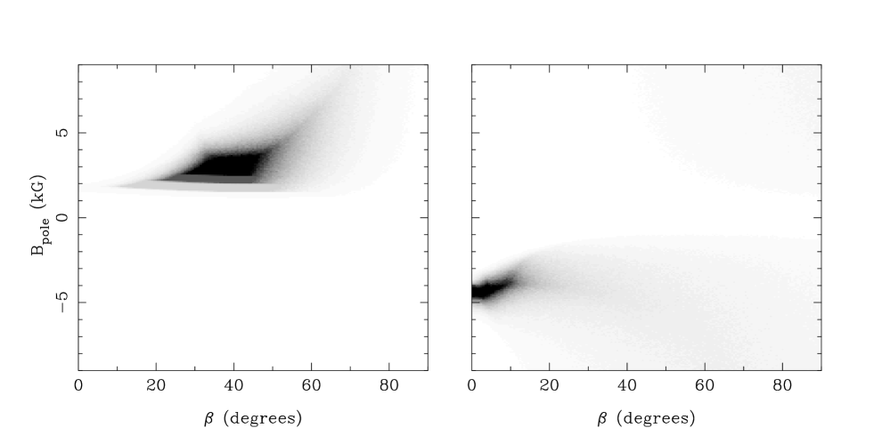
Figure 3: Kolmogorov-Smirnov statistics for BP Tau (left) and DF Tau (right). Each pixel shows the probability that the observations are consistent with a simulated distribution of measurements from a dipole magnetic field with given values of $B_{\mathrm{pole}}$ and dipole offset ($\beta$). Black represents a probability of $>50$ per cent, white is $0$, and the greyscale shows a linear range between these two values. The step changes seen in the BP Tau simulation are a consequence of employing the K-S test with a small number of data points.

Many such sets of observations were simulated for varying values of $B_{\mathrm{pole}}$ and $\beta$ and a Kolmogorov-Smirnov (K-S) test was carried out to determine whether the genuine observations were consistent with the simulated distribution. In Fig.3, the K-S probability is shown as $B_{\mathrm{pole}}$ and $\beta$ are changed, and it can be seen that the models are ruled out for many combinations of the these parameters. In each case, there is a practical constraint that $B_{\mathrm{pole}}$ must be at least as great in magnitude as the maximum observed value of $B_{z}$. Imposing a narrow range of viewing inclinations will also introduce a degeneracy between $B_{\mathrm{pole}}$ and $\beta$, i.e. a $B_{\mathrm{pole}}$ value that does not match the star’s actual $B_{\mathrm{pole}}$ might be compensated for by changing the dipole offset so that the distribution of simulated observations is more widely spread and then is consistent with the real observations.

The BP Tau observations are found to be best matched by $B_{\mathrm{pole}}\sim 3$ kG and $\beta\sim 40\degr$. DF Tau was consistent with $\sim-4.5$ kG and $\beta<\sim 10\degr$ – the difference in dipole offset is consistent with our expectation, since our model gives smaller dipole offsets for objects with smaller variability for obvious physical reasons.

4 Conclusions

Measurements were made of the mean longitudinal magnetic field, $B_{z}$, from Zeeman splitting of the He i $\lambda 5876$ line in the spectra of seven classical T Tauri stars. For the star that had been previously best-studied with this technique, BP Tau, the field strengths were mostly within the range found by previous authors (Johns-Krull et al., 1999; Valenti et al., 2003), but we also measured the strongest field so far detected for any T Tauri star (4 kG). Another star, DF Tau, was found to have a magnetic field that was also within the range of previous measurements. A first $B_{z}$ detection was made for DN Tau, and the stars GM Aur and RW Aur each showed one measurement that was above our instrumental sensitivity limit. In total, five of the seven targets showed evidence for a magnetic field at one or more epochs.

There are now a total of nine CTTSs in the literature with precise magnetospheric field measurements, and of this sample a statistically significant field has been detected in seven objects. Interestingly our repeat observations of BP Tau and DF Tau indicate that the fields may have characteristics that are persistent on a time-scale of years (i.e. hundreds of rotation cycles). It is evident that classical T Tauri stars have fields with the magnitude ($\sim 1$ kG) and stability expected in theoretical studies of the magnetospheric accretion process (e.g. Romanova et al. 2003).

We note that the dipole offset estimates derived for BP Tau and DF Tau (40°and $<10$°respectively) would result in very different magnetospheric stream structures according to the magneto-hydrodynamical models of Romanova et al. (2003). The simulations suggest that DF Tau should accrete from two diametrically opposed streams, while BP Tau (with its larger dipole offset) would have a more complex accretion structure. However, it appears BP Tau shows line profile variability that is consistent with an inclined dipole (Gullbring et al. 1996), while the variability of DF Tau is apparently difficult to interpret in terms of the magnetospheric accretion paradigm (Johns-Krull & Basri 1997).

The next stage of these investigations should be a simultaneous measurement of the mean field and the longitudinal field, perhaps using time-series measurements to map the surface magnetic field structure using a technique such as Zeeman Doppler Imaging (ZDI; Semel 1989).

References

- Babcock (1947) Babcock H. W., 1947, ApJ, 105, 105
- Basri et al. (1992) Basri G., Marcy G. W., Valenti J. A., 1992, ApJ, 390, 622
- Bouvier (1990) Bouvier J., 1990, AJ, 99, 946
- Bouvier et al. (1986) Bouvier J., Bertout C., Bouchet P., 1986, A&A, 158, 149
- Bouvier et al. (1993) Bouvier J., Cabrit S., Fernandez M., Martin E. L., Matthews J. M., 1993, A&A, 272, 176
- Chen et al. (1990) Chen W. P., Simon M., Longmore A. J., Howell R. R., Benson J. A., 1990, ApJ, 357, 224
- Cohen & Kuhi (1979) Cohen M., Kuhi L. V., 1979, ApJ, 227, L105
- Collier Cameron & Campbell (1993) Collier Cameron A., Campbell C. G., 1993, A&A, 274, 309
- Edwards et al. (1994) Edwards S., Hartigan P., Ghandour L., Andrulis C., 1994, AJ, 108, 1056
- Guenther et al. (1999) Guenther E. W., Lehmann H., Emerson J. P., Staude J., 1999, A&A, 341, 768
- Gullbring et al. (1998) Gullbring E., Hartmann L., Briceno C., Calvet N., 1998, ApJ, 492, 323
- Gullbring et al. (1996) Gullbring E., Petrov P. P., Ilyin I., Tuominen I., Gahm G. F., Loden K., 1996, A&A, 314, 835
- Hartigan et al. (1995) Hartigan P., Edwards S., Ghandour L., 1995, ApJ, 452, 736
- Hartmann et al. (1994) Hartmann L., Hewett R., Calvet N., 1994, ApJ, 426, 669
- Hartmann & Stauffer (1989) Hartmann L., Stauffer J. R., 1989, AJ, 97, 873
- Hill et al. (1998) Hill G. M., Bohlender D. A., Landstreet J. D., Wade G. A., Manset N., Bastien P., 1998, MNRAS, 297, 236
- Hirth et al. (1994) Hirth G. A., Mundt R., Solf J., Ray T. P., 1994, ApJ, 427, L99
- Johns-Krull & Basri (1997) Johns-Krull C. M., Basri G., 1997, ApJ, 474, 433
- Johns-Krull et al. (1999) Johns-Krull C. M., Valenti J. A., Hatzes A. P., Kanaan A., 1999, ApJ, 510, L41
- Johns-Krull et al. (2001) Johns-Krull C. M., Valenti J. A., Saar S. H., Hatzes A. P., 2001, in Garcia Lopez R. J., Rebolo R., Zapaterio Osorio M. R., eds, ASP Conf. Ser. 223: 11th Cambridge Workshop on Cool Stars, Stellar Systems and the Sun, Astron. Soc. Pac., San Francisco . p. 521