Large-scale variations of the dust optical properties in the Galaxy

We present an analysis of the dust optical properties at large scale, for the whole galactic anticenter hemisphere. We used the 2MASS Extended Source Catalog to obtain the total reddening on each galaxy line of sight and we compared this value to the IRAS 100 $\mu$m surface brightness converted to extinction by Schlegel et al. (1998). We performed a careful examination and correction of the possible systematic effects resulting from foreground star contamination, redshift contribution and galaxy selection bias. We also evaluated the contribution of dust temperature variations and interstellar clumpiness to our method. The correlation of the near–infrared extinction to the far–infrared optical depth shows a discrepancy for visual extinction greater than 1 mag with a ratio $A_{V}({\rm FIR})/A_{V}({\rm gal})=1.31\pm 0.06$. We attribute this result to the presence of fluffy/composite grains characterized by an enhanced far–infrared emissivity. Our analysis, applied to half of the sky, provides new insights on the dust grains nature suggesting fluffy grains are found not only in some very specific regions but in all directions for which the visual extinction reaches about 1 mag.

1 Introduction

Large scale dust studies started with IRAS which revealed the whole sky in four far–infrared (FIR) wavelength bands. It led to the current view of the interstellar dust seen as a 3 components grain population (Désert et al., 1990): polycyclic aromatic hydrocarbons (PAH), very small grains (VSG) and big grains (BG). The color analysis of IRAS surface brightnesses provides insight to the variations of the 3 dust component abundances with respect to various environments. BG dominate in molecular clouds whereas VSG are more representative of the diffuse interstellar medium usually associated with the atomic hydrogen. Our understanding of interstellar medium (ISM) dust has further evolved with advances in FIR and submillimeter (submm) instrumentation in the last decade. Not only is the dust composed of different grain size components but the optical properties of the dust change with the environment. The PRONAOS balloon observations reveal the complexity of the dust properties with emissivity variations (Bernard et al., 1999; Stepnik et al., 2003) and spectral index variations (Dupac et al., 2002). More difficult because of the atmosphere absorption but still possible, ground based observations in the submillimeter range also find evidence of dust emissivity variations with SCUBA observations (Johnstone et al., 2003). The initial results from IRAS, DIRBE, or ISO, which were mainly focused on dust abundances and temperature, reveal much more if re-examined in light of these recent dust optical property results obtained from longer wavelengths, notably in the submm. Cambrésy et al. (2001) have quantified the emissivity enhancement at 100 $\mu$m comparing COBE/DIRBE with an extinction map of the Polaris Flare. Their results have been confirmed by del Burgo et al. (2003) who found similar behavior for the FIR dust emissivity in eight nearby interstellar regions observed by ISOPHOT. Dale & Helou (2002) studied a sample of galaxy spectral energy distributions with ISO and IRAS, proposing a change in the dust emissivity at wavelengths longer than 100 $\mu$m to match SCUBA brightnesses. ISOPHOT sources discovered at 200 $\mu$m (but not detected at 100 $\mu$m) suggest a change in the grain properties (Lehtinen et al., 2003).

Although it is now established that the dust optical properties vary with the environment, likely due to fluffy grain population, the spatial extent in these variations is still controversial and the density threshold for the transition from regular to the enhanced emissivity dust population remains unknown. In this paper we address these questions using a large scale analysis of the whole galactic anticenter hemisphere. We propose to compare data from IRAS and DIRBE, converted to dust extinction by Schlegel et al. (1998) (hereafter SFD98), with the reddening of 2MASS galaxies. Our goal is to investigate the dust properties through the apparent discrepancy between these two quantities. The 2MASS extended source catalog characteristics are presented in Sect. 2 followed by a detailed analysis of the biases in the galaxy color excesses in Sect. 3. Section 4 is dedicated to the analysis of the correlation between the galaxy reddening and the FIR dust opacity, the conclusions of the paper are presented in Sect. 5.

2 The 2MASS extended source catalog

2.1 Presentation

The 2MASS All-Sky Data Release for extended sources (XSC) contains positions and photometry in $JHK_{s}$ for 1.6 million objects (Jarrett et al., 2000a). About 97% are galaxies but the catalog also contains galactic resolved sources such as HII regions, planetary nebulae, reflection nebulae, young stellar objects, etc. Galaxies were identified using a decision tree method which uses several parameters including size, shape, central surface brightness and color. In order to increase the reliability of the object classification, a visual classification has also been performed. It is mainly based on the eye examination of the color-combined images, but also optical DSS images when it was needed. Roughly 25-30% of all XSC sources have been inspected, with close to 100% for bright sources ($K_{s}<12.5$ mag, Cutri et al., 2003). All XSC sources have been inspected in the galactic plane ($|b|<5\deg$) and in some other regions of specific interest (Magellanic clouds, galaxy clusters like Virgo). Visual inspection reveals that only a small fraction (less than 1%) of sources are artifacts of various origins such as bright star neighborhood, airglow, meteor streaks or image edges. In total, among the $\sim 1.5\times 10^{6}$ galaxies in the XSC, more than $3\times 10^{5}$ have been confirmed by eye.

2.2 Catalog properties

2.2.1 Source density and completeness

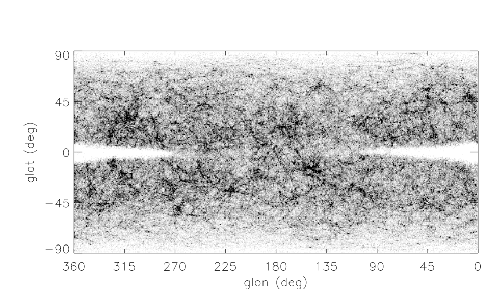
Figure 1: Spatial distribution of the $1.5\times 10^{6}$ 2MASS galaxies projected in rectangular coordinates. Milky Way objects have been removed. The Cartesian projection is in galactic coordinates and is centered at the anticenter direction. The absence of detected galaxies near the galactic center results from the confusion noise due to high stellar densities.

Figure 1 shows the spatial distribution of the XSC galaxies, filtered from the Milky Way extended sources. The large scale structures of the universe dominate the source distribution over the local dust extinction. The confusion noise prevents the galaxy identification in the very high stellar density regions such as the Galactic Center (Jarrett et al., 2000b). The striking filamentary structure in the source distribution reflects the large scale structure of galaxies in the universe (see also Jarrett, 2004). It is worth noting that if Fig. 1 were restricted to a longitude range of 90 to 270 deg (i.e. the anticenter hemisphere), the Milky Way disk would barely be seen. We will therefore not consider using source counts in the near–infrared as an extinction estimator as it has been done by Burstein & Heiles (1982) in the visible. Since the source counts are incomplete in the Galactic Center region, the analysis presented in this paper is restricted to the anticenter hemisphere, about $8.5\times 10^{5}$ galaxies.

Figure 2: Magnitude distribution of galaxies at $J$ (upper panel) and $K_{s}$ (lower panel) for latitudes greater than 25 deg and lower than 5 deg. Only sources in the galactic anticenter hemisphere (longitude from 90 to 270 deg) are considered.

In the following, magnitudes always refer to the fiducial elliptical isophotal ($K_{s}=20$ mag arcsec^-2) magnitudes. The level of completeness for the detection depends on the latitude as the stellar density increases in the plane. Magnitude distributions for $|b|>25\deg$ and $|b|<5\deg$ are presented in Fig. 2 (Jarrett et al., 2000b). The low and high latitude samples are quite similar. The latitude has only a small impact on the value of the turn off in the distribution which represents the 2MASS sensitivity limit for extended objects. The low-latitude distribution is almost parallel to the high-latitude curve, indicating the confusion noise reduces the completeness at all magnitudes (except the very bright end, $J<9$) without any significant change in the observed luminosity function shapes. Consequently, we do not expect any significant color systematic effect from photometry signal-to-noise.

2.2.2 Galaxy colors

The color distribution of galaxies is related to their morphological type. It reflects various characteristics such as the stellar content (old/young populations, star forming rate) and the dust fraction. Jarrett (2000) and Jarrett et al. (2003) analyzed 2MASS galaxy properties according to their morphological types and found that ellipticals are slightly redder in near–infrared color than lenticulars and that normal barred and transition barred spirals have similar colors. However the dispersion for spirals is increased by a factor of 2, going from early to late type due to important star formation and amount of dust material in the earliest types. For some morphologies, color can be clearly different as for AGN which are 0.3-0.4 mag redder than the average, or dwarf, irregular/peculiar and compact galaxies which are bluer than the norm. Ellipticals and spirals dominate the galaxy population and we find $J-K_{s}=1.0\pm 0.1$ for high-latitude galaxies (no Milky Way extinction) restricted to $J<14.0$ and $K_{s}<13.3$. These magnitude cuts are addressed later in the paper and correspond to our high-latitude sample as shown Fig. 6.

3 Extinction from galaxy colors

The extinction estimation is based on the $J-K_{s}$ galaxy color excess from the normal distribution. Visual extinction is derived from the color excess $E_{J-K_{s}}$ as follows:

$$E_{J-K_{s}} = (J-K_{s})_{\rm obs}-(J-K_{s})_{\rm int}$$

$$A_{V} = \left(\frac{A_{J}}{A_{V}}-\frac{A_{K_{s}}}{A_{V}}\right)^{-1}E_{J-K_{s}}$$

where the indices $obs$ and $int$ stand for $observed$ and $intrinsic$, respectively. $(J-K_{s})_{\rm int}=1.0\pm 0.1$ mag assuming zero redshift. We use the extinction law from Rieke & Lebofsky (1985) for which $A_{J}/A_{V}=0.282$ and $A_{K_{s}}/A_{V}=0.112$ yielding the color excess to visual extinction conversion formula $A_{V}=5.88\times E_{J-K_{s}}$. Although the determination of the extinction looks straightforward, systematic effects might occur and must be overcome. We distinguish three independent possible effects:

• contamination of the photometry by foreground stars

• color of a galaxy affected by its redshift.

• selection effect with the galactic latitude.

The following section explores all the possible bias that may contaminate the galaxy colors.

3.1 Biases in the reddening estimation

3.1.1 Foreground star contamination

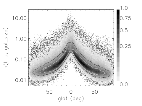
Figure 3: Density plot of the number of foreground stars from a Monte Carlo simulation. The contamination probability depends on the latitude, the longitude (from 90 to 270 deg) and the galaxy size which are taken from the XSC. The y-axis is in log scale and the bar scale indicates the normalized density color coding. As an example, for a galaxy at $b=10$ deg, the number of foreground stars is between 0.04 and 6 (depending on longitude and galaxy size) and the most common number is about 0.2 star (within the 50% iso-contour).

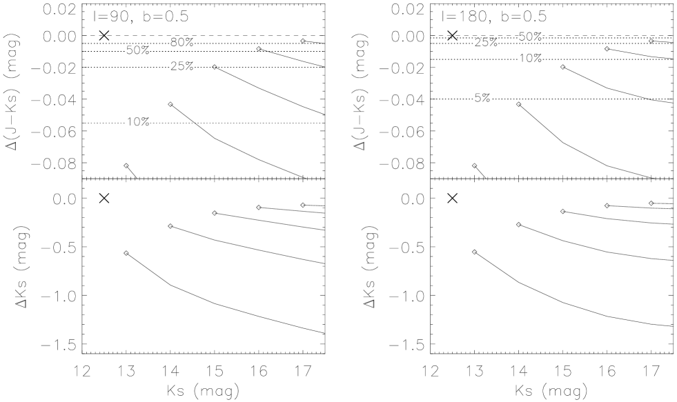
Figure 4: $J-Ks$ color contamination (upper panel) and $K_{s}$ contamination (lower panel) of a typical galaxy ($K_{s}=12.5$, with a 12″ diameter) by foreground stars in the galactic plane for $l=90$ deg (left) and $l=180$ deg (right). In all panels, the cross represents the reference galaxy and the diamonds the brightest foreground star. Solid lines show the contamination level versus the magnitude of the foreground stars. For the upper panels, dotted lines give the probability of reaching the corresponding contamination level.

The probability of having a star on a galaxy line of sight depends on the galaxy size and the local stellar number density. The first parameter introduces a systematic effect because galaxies of a given size are not randomly spread over the sky but often concentrate in clusters which are groups of same distance, and thus similar size, objects. The latter parameter, the stellar number density, relies mostly on the galactic latitude or the star distribution in the disk of the Milky Way. The foreground contamination biases the galaxy photometry toward the blue because stars are generally bluer than galaxies with an average $J-K_{s}$ color of $\sim 0.65$ versus $\sim 1.0$ (see Sect. 2.2.2). However, if the star is bright enough compared to the galaxy it is likely identified and its contribution to the total flux is subtracted (Jarrett et al., 2000a). The contamination arises for stars more than 1 magnitude fainter than the galaxy. A Monte Carlo simulation is well adapted to estimate the bias. We use the following parameters:

• $\;\left[J({\rm gal})+1\right]\;<J({\rm star})\;<19.0$ and $\left[K_{s}({\rm gal})+1\right]<K_{s}({\rm star})<17.5$. Fainter sources comprise the uniform background level (i.e. background fluctuations).

• galaxy size and local stellar number density for $K_{s}<14$ from the XSC catalog.

• star luminosity function slope (to extrapolate the number of star fainter than $K_{s}=14$): 0.31

• $\overline{J-K_{s}}$ from 0.65 mag for stars at high galactic latitude to 0.98 mag at $b=0$ were diffuse extinction is not negligible and reddening is appreciable.

Figure 3 shows the number of foreground stars for each galaxy versus the galactic latitude. Using this number, the stellar luminosity function and the magnitude limit for stars mentioned previously we removed the stellar component in the flux of each galaxy. The level of contamination is globally small since less than 1% of the galaxies have at least 1 foreground star. For latitude higher than 25 deg or lower than 5 deg the fraction of contaminated galaxies is 0.09% and 1.5%, respectively. An example of how the foreground star contamination translate into magnitude and color bias is presented in Fig. 4. It shows the contamination of a galaxy, $K_{s}=12.5$, with a 12″ diameter. To compute the probability of presence of a foreground star we use the starcount model described in Jarrett (1992) and Jarrett et al. (1994), with validation analysis presented in Cambrésy et al. (2002). The model also provides us with the luminosity function at a given latitude and longitude. For the worst case, at $l=90$ and $b=0.5$, the contamination could reach a few percent of a magnitude in color (about 25% probability that $\Delta(J-K_{s})>0.02$ mag). At this stage a new catalog is generated with the statistical correction of the foreground star contamination bias. With this correction, we expect color biases to be smaller than 1 to 2%.

3.1.2 Redshift contribution

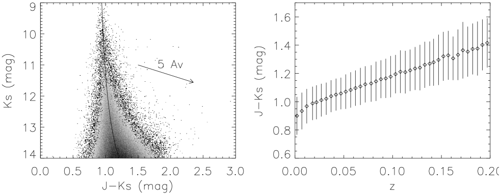
Figure 5: Left panel: color-magnitude diagram for galaxies non-reddened by the ISM ($I_{100\mu{\rm m}}<1.5$ MJy sr^-1). The solid line indicates the magnitude-dependent reference for the extinction measurements. It is defined by the equation $J-K_{s}=(16.5-K_{s})^{-1}+0.81$. Right panel: K-correction for $J-Ks$ from Jarrett (2004). The color variation in our galaxy sample is consistent with a maximum redshift of about 0.1.

Given the 2MASS pixel size, galaxies as small as 10″ are resolved as extended sources, reaching $z\sim 0.1$ for the most luminous cluster members (Jarrett, 2004). At this redshift level, more $H$-band stellar light is transfered into the $K_{s}$-band, reddening the $J-K_{s}$ galaxy color. If individual redshifts for each source were known the method would be to apply the K-correction to obtain the photometry that would have been measured at $z=0$. However we are unable to make this correction as long as we do not have the individual redshift knowledge. It is still possible to correct the bias using the color-magnitude diagram presented in Fig. 5. The subsample selected to make this diagram contains only the object with a line of sight characterized by an IRAS 100 $\mu$m surface brightness lower than 1.5 MJy sr^-1. The low 100 $\mu$m surface brightness ensures that the line of sight is free from local ISM reddening. Assuming the fainter objects are the most distant observed, the Fig. 5 trend is directly related to the K-correction. The diagram shows a reddening of $J-K_{s}\sim 0.2$ mag between the bright and the faint end of the magnitude distribution which is in agreement with the value expected for $z\sim 0.1$. The color excess used to derive the extinction is therefore defined in the color-magnitude plane as the distance along the reddening vector between each galaxy and the reference line of equation $J-K_{s}=(16.5-K_{s})^{-1}+0.81$ (Fig. 5). The color excess is determined for each galaxy following this definition. The statistical uncertainty on this correction is negligible compared to the photometric uncertainty which causes the scatter in Fig. 5.

3.1.3 Selection effect with the galactic latitude

Figure 6: Latitude-dependent limiting magnitude used to correct the selection effect of galaxies reddened by the Milky Way disk dust. The curves represent the loss in sensitivity due to confusion noise.

Galaxies detected through the Milky Way disk suffer from more extinction than high-latitude objects. Consequently the nature of the faint galaxies depends on the latitude. For instance more high redshift objects are detected at high latitude. This has been corrected in the redshift bias analysis, but one can imagine other selection effect such as a low surface brightness galaxy fraction or a face-on galaxy fraction as a function of the galactic latitude. Another possible effect related to foreground extinction make the fainter outer parts of galaxies to fall below the isophotal detection limit. These outer parts are usually bluer because of the age and metallicity gradients. The non-detection of the outer parts would make the galaxy color to appear redder and the derived extinction to be overestimated. The resulting bias depends on the photometric bands used. For $J-K_{s}$, Jarrett et al. (2003) provide radial profile for about 500 large 2MASS galaxies showing the color gradient is actually small (see their Fig. 15). The color change is about 0.1 mag from the galaxy center to the outer disk, where most of the change is happening well within the half-light radius. To reduce the selection effects we evaluate the average extinction as a function of the latitude and we set a limiting magnitude which depends on the galactic latitude. Figure 6 shows that the magnitude cut is about 1 mag brighter at $b>30$ deg than it is at $b=0$ deg. The difference in $K_{s}$ is smaller with about 0.4 mag. It is a strong constraint on the total galaxy number which is reduced from $8.5\times 10^{5}$ to $1.2\times 10^{5}$ galaxies.

3.2 Extinction mapping

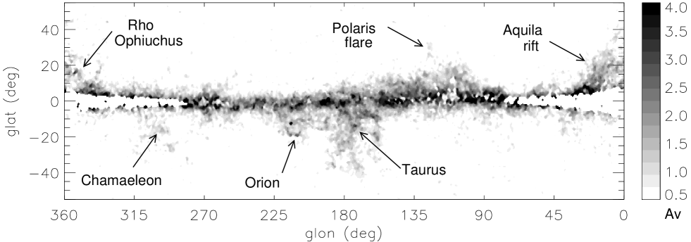
Figure 7: Extinction map derived from the median color in adaptive cells containing 5 galaxies each. The scale is labeled in visual magnitude units. The statistical uncertainty is 0.3 mag. As for Fig. 1 no galaxy is detected near the galactic center due to high stellar density.

It is clear from Fig. 1 that the galaxy density variations follow the large scale structure of the universe (see also Jarrett, 2004). The adaptive method described in Cambrésy et al. (2002) to derive the extinction is particularly well adapted in this case. For each position in the map the extinction is obtained from the median color excess of the 5 closest neighbors. This technique optimizes the spatial resolution to the local galaxy density. The result is presented in Fig. 7. The average spatial resolution is 1 deg with variation from 30′ in large scale structures to about 4 deg for isolated galaxies. Such a low resolution map should be viewed with caution since galaxies are not uniformly distributed in space. As mentioned Sect. 2.2.2 the galaxy color for a non-obscured field is $J-K_{s}=1.0\pm 0.1$. It translates into a statistical uncertainty for the visual extinction of $0.1\times(A_{J}/A_{V}-A_{K_{s}}/A_{V})^{-1}/\sqrt{5}=0.3$ mag. However the systematic error resulting from the spatial non-uniformity of the galaxy distribution probably dominates the error. The extinction map obtained from galaxy color excess is not equivalent to an average extinction at the given resolution. The extinction map presented in Fig. 7 should actually be considered as a lower limit for the extinction since galaxies are preferentially detected in low extinction areas, i.e. between dense clouds that block the light coming from low surface brightness objects.

4 Extinction and FIR dust opacity comparison

4.1 Individual line of sight analysis

Our goal is to compare the extinction measured from 2MASS galaxy color with the dust optical depth in the FIR. IRAS data provides the 100 $\mu$m flux density. The temperature is needed to translate the thermal dust emission to optical depth. The work has been done by SFD98 using IRAS data modified to take into account the temperature variations derived from lower resolution DIRBE data. They have carried out the next step which is the conversion of the optical depth into visual extinction. Since they performed a careful calibration at high galactic latitude, we use their dust map.

The previous section pointed out that the extinction map presented in Fig. 7 is not equivalent to an average extinction at the cell resolution. The situation is different for the FIR surface brightness maps which provide the true arithmetic mean value at the beam resolution. The direct comparison of the two maps is therefore not appropriate. As an alternative to a map to map comparison we propose a strategy which consists in comparing directly the individual galaxy reddening to the corresponding SFD98 pixel extinction map. Dutra et al. (2003a) used a similar strategy focusing on 20 early type galaxies for which they could derive the extinction from their individual spectra. In the individual comparison of galaxies with the SFD98 pixels, the spatial resolution problem is reversed and single galaxies have the higher resolution with a typical resolution of about 10″ (the size of a galaxy) where the IRAS beam size is only $\sim 5\arcmin$.

4.1.1 Temperature bias

The existence of several dust temperature components has been revealed by IRAS through the analysis of the correlation between the 100 $\mu$m and 60 $\mu$m surface brightnesses (Laureijs et al., 1991; Abergel et al., 1994). These results are actually based on the observation of changes in the small grain abundances (Boulanger et al., 1990). In Lagache et al. (1998) the temperature variations are directly measured using FIRAS spectra and DIRBE maps. They found a dust temperature of about 17.5 K for the diffuse ISM and a colder component at around 15 K or less towards molecular clouds.

Figure 8: Figure from Cambrésy et al. (2001) representing the effective to total optical depth ratio as a function of the warm component fraction. Cold and warm components are described by the modified Planck function $P=B_{\nu}(T)\times(\lambda/\lambda_{0})^{-2}$ with $T_{c}=13.5$ K and $T_{w}=17.5$ K.

In SFD98, the FIR optical depth is derived from the IRAS 100 $\mu$m brightness using an effective temperature for a line of sight. It is not equivalent to the sum of the optical depths from different temperature components. The impact of this point on the final optical depth is discussed in Cambrésy et al. (2001) with a model assuming the 100 $\mu$m emission comes from a mixture of two distinct components. Assuming a $\nu^{2}$ emissivity law, a single black body and a combination of two black bodies are fitted to the emission. The result is presented in Fig. 8, which shows the effective optical depth is always smaller than the sum of the optical depth for the two dust components. When temperature changes along a line of sight, SFD98 are expected to underestimate the amount of interstellar material. On the other hand, the temperature variations have absolutely no effect on the galaxy reddening. There is a bias in the SFD98 optical depth determination which depends on the fraction of warm dust component along a line of sight. This fraction is hard to estimate and according to the modeling of Fig. 8 a 5 to 15% underestimation in the SFD98 extinction is possible.

4.1.2 ISM clumpiness bias

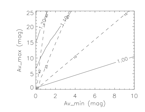
Figure 9: ISM clumpiness bias derived from a synthetic molecular clouds (Padoan et al., 1998). The solid lines are the isocontours for $\overline{A_{V}}/A_{V}({\rm gal})$ and the dashed lines correspond to the $\sigma(A_{V})/A_{V}$ ratio isocontours labeled in percentage. For $\sigma(A_{V})/A_{V}\approx 25\%$, the bias in the extinction determination $(\overline{A_{V}}-A_{V}({\rm gal}))/A_{V}({\rm gal})$ is less than 10%.

Section 3.2 focuses on the role of the galaxy distribution in the extinction estimation and shows a non-linear effect results from the non-uniform galaxy distribution. It is still relevant here because we compare each galaxy to the corresponding IRAS pixel which is about 5′ large. If the interstellar medium is clumpy at the IRAS scale we expect a systematic effect since galaxies will preferentially be detected in the less obscured part of the pixel whereas the FIR extinction relies on the arithmetic mean over the pixel. Lada et al. (1999) and Thoraval et al. (1997) have discussed the dust clumpiness and they both conclude it is rather smooth compared to the gas. On small scale they propose an upper limit for the $\sigma(A_{V})/A_{V}$ ratio of about 25%. The $\sigma(A_{V})/A_{V}$ ratio is a constraint on the dust distribution but the scaling function is also needed to compute the bias. Padoan et al. (1998) generate synthetic molecular clouds from supersonic turbulence. We use a sample of unreddened galaxies together with their simulation to compute the bias. The method consists in applying the extinction from the simulation and then to apply a magnitude cut which is equivalent to the instrumental sensitivity limit. Then the ratio of the arithmetic mean extinction to the median extinction from the remaining galaxies gives the bias. We applied this method to various values for the minimum and maximum extinction values in the simulated cloud; results are presented in Fig. 9. For each run the $\sigma(A_{V})/A_{V}$ ratio is computed and constrains the fluctuations expected from small scales. For $\sigma(A_{V})/A_{V}\approx 25\%$ the galaxy color excess underestimates the average extinction by about 10% if the real extinction goes from 3 to 20 mag within a single IRAS pixel. For lower extinctions, the systematic effect decreases. It is safe to consider a 10% bias as an upper limit.

4.2 Results

Figure 10: Upper panel: difference of extinction between SFD98 and 2MASS galaxies versus the galaxy extinction, restricted to SFD98 pixels not contaminated or corrected for point sources (=covered by the PSCz catalog). The deviation for $A_{V}>1$ is fitted by the dashed line of equation $A_{V}({\rm FIR})=1.31\times A_{V}({\rm gal})-0.24$. Lower panel: same as upper panel but with all SFD98 pixels, including those for which the contamination cannot be assessed. The dashed line is $A_{V}({\rm FIR})=1.58\times A_{V}({\rm gal})-0.66$

Figure 11: Extinction from 2MASS galaxies (solid line) and from SFD98 (dashed line) versus the galactic latitude cosecant for the northern (upper panel) and the southern (lower panel) part of the anticenter hemisphere. The sample is restricted to SFD98 pixels not contaminated or corrected for point sources (=covered by the PSCz catalog).

Our sample contains $1.2\times 10^{5}$ galaxies corrected for all biases described in Sect. 3.1. To compare the extinction obtained for each galaxy with the FIR extinction map pixels we proceed as follows: the two quantities are averaged on 1 deg wide strips in latitude that cover the whole anticenter hemisphere longitude range (from 90 to 270 deg). Almost all the spatial information is lost in this operation except the latitude. Point sources contaminate the IRAS fluxes. To derive their extinction map Schlegel et al. (1998) used the PSCz catalog (Saunders et al., 2000) to remove the point sources brighter than 0.6 Jy at 60 $\mu$m over most of the sky at $|b|>5$ deg and over parts of the sky at lower latitudes. The low-latitude sky is critical in our analysis and we adopt a conservative approach. Among the 1149 low-latitude IRAS pixels ($0.5<b<1.5$ deg) containing a 2MASS galaxy the contamination can be assessed for only for 259 (=23%) of them. The upper panel of Fig. 10 shows the extinction difference between SFD98 and 2MASS galaxies versus the galaxy extinction for pixels not contaminated or corrected for point sources, i.e. in the area covered by the PSCz catalog. For extinction greater than 1 mag a linear fit gives $A_{V}({\rm FIR})/A_{V}({\rm gal})=1.31\pm 0.06$. The lower panel is similar but includes all pixels, which means pixels not contaminated or corrected for point sources and pixels for which the contamination cannot be assessed. The ratio $A_{V}({\rm FIR})/A_{V}({\rm gal})$ becomes 1.58. The discrepancy with the previous value is significant. We chose to be conservative keeping only pixels covered by the PSCz catalog which represent 23% of our galaxy sample at $|b|<5$ deg and almost the whole sky at $|b|>5$ deg. However pixels actually contaminated in the low-latitude regions of the PSCz catalog represent only 7% of the population. It suggests we are probably underestimating the $A_{V}({\rm FIR})/A_{V}({\rm gal})$ ratio which would be in the range from 1.31 to 1.58.

Figure 11 presents the same data in another form. It shows $A_{V}$ versus the latitude cosecant. The discrepancy appears more clearly in the south because extinction is more significant in this area with the large envelope surrounding the Taurus cloud.

4.3 Discussion

It is now understood that the SFD98 map overestimates the extinction at least in some specific regions that have been carefully examined by various authors. For instance Arce & Goodman (1999) deduced an overestimation factor for SFD98 of 1.3 to 1.5 in the Taurus clouds, Chen et al. (1999) obtained a 1.16 average factor towards 131 globular clusters at $|b|>2.5$ deg. A factor of 2 was found by Cambrésy et al. (2001) in the Polaris Flare which is a peculiar region with an unexpected low temperature for a cirrus. In the galactic center direction a discrepancy factor from 1.31 to 1.45 have been measured using 2MASS data (Dutra et al., 2003b, 2002). In a recent paper Dutra et al. (2003a) studied the spectral properties of 20 early-type galaxies located at $|b|<25$ deg to derive the extinction along the line of sight. They found a ratio $A_{V}({\rm FIR})/A_{V}({\rm gal})\approx 1.31$ for $A_{V}>0.75$ and an agreement for lower values. Although their sample contains only 20 objects they benefit from the high reliability of spectra. Our analysis yields a very similar conclusion on a large scale with a sample of $1.2\times 10^{5}$ galaxies. Dutra et al. (2003a) and Arce & Goodman (1999) suggest the SFD98 map should be recalibrated, but they do not propose any physical reason for this adjustment.

We support the idea of an enhanced emissivity of the dust in the FIR due to fluffy grains (Cambrésy et al., 2001; Stepnik et al., 2003). A grain growth through grain-grain coagulation or accretion of gas species is expected in dense cold molecular clouds (Draine, 1985) and leads to porous grains. Dwek (1997) studied the fluffy grain optical properties and showed the emissivity in the FIR is increased for porous grains. If this effect applies to the present analysis it means the grain coagulation starts at extinction close to 1 mag. We would expect variations from cloud to cloud depending on their star forming activity, the local interstellar radiation field and their geometry. The minimum extinction value at which the FIR to extinction ratio changes is actually not the correct quantity to check since it relies on the column density rather than the 3D volume density. Several low density clouds on the same line of sight and a single dense cloud may have the same column density but their $A_{V}({\rm FIR})/A_{V}({\rm gal})$ would be very different. However, Fig. 11 points out the extinction values beyond the threshold for the enhanced emissivity are generally restricted to low-latitude regions with $|b|<8$ deg. Our interpretation for the grain aggregate formation leads to the conclusion that higher-density clouds are preferentially located in the plane, which is in total agreement with our knowledge about the ISM distribution in the Galaxy. A comparative analysis for various environment would confirm our hypothesis if clouds were proved to be different in their FIR to extinction correlation. Unfortunately the spatial information in our analysis, the galactic latitude, does not allow us to conclude on spatial variation of the $A_{V}({\rm FIR})/A_{V}({\rm gal})$ ratio.

5 Conclusion

The 2MASS galaxy colors appears to be a very interesting extinction estimator to compare with FIR extinction. Both extinction estimators are sensitive to the absorption for the whole line of sight, but they are totally independent. We have investigated the galactic anticenter hemisphere and found $A_{V}({\rm FIR})/A_{V}({\rm gal})=1.31\pm 0.06$ for the SFD98 extinction map restricted to pixels corrected for point source contamination. We correct for several biases that would affect the correlation analysis. The foreground star contamination estimated with the stellar density number and the galaxy size has been found negligible with about 1-2% uncertainty. Redshifted galaxy photometry has been corrected using a color-magnitude diagram. The correction is consistent with the expected K-correction for $z\la 0.1$. The presence of several dust temperature components on a line sight implies a systematic effect in the FIR extinction map. This effect yields a 5 to 15% underestimation of the FIR extinction which reduces the discrepancy between FIR and galaxy color extinction. The difference in the spatial resolution of the extinction value (6.1′ for SFD98 and $\sim 10\arcsec$ for 2MASS galaxies) roughly compensates the temperature systematics because of the ISM clumpiness.

In this paper we have generalized previous studies that had already concluded the SFD98 map overestimates the extinction for some specific directions to half of the sky. At large scale the discrepancy appears for $A_{V}\ga 1$, suggesting the whole galactic disk is affected. We attribute our result to the presence of fluffy/composite grains which have an enhanced emissivity in the FIR. Our large scale study suggests they are more common that previously thought since they would be formed even at low extinction and not only in dense cold clouds. More analysis are needed to confirm this point especially to recover more spatial information. Complementary FIR and submm data from Spitzer, Herschel and Planck are expected to solve this problem by providing dust spectra at long wavelengths.