The ACS Virgo Cluster Survey IV: Data Reduction Procedures for Surface Brightness Fluctuation Measurements with the Advanced Camera for Surveys

Abstract

The Advanced Camera for Surveys (ACS) Virgo Cluster Survey is a large program to image 100 early-type Virgo galaxies using the F475W and F850LP bandpasses of the Wide Field Channel of the ACS instrument on the Hubble Space Telescope (HST). The scientific goals of this survey include an exploration of the three-dimensional structure of the Virgo Cluster and a critical examination of the usefulness of the globular cluster luminosity function as a distance indicator. Both of these issues require accurate distances for the full sample of 100 program galaxies. In this paper, we describe our data reduction procedures and examine the feasibility of accurate distance measurements using the method of surface brightness fluctuations (SBF) applied to the ACS Virgo Cluster Survey F850LP imaging. The ACS exhibits significant geometrical distortions due to its off-axis location in the HST focal plane; correcting for these distortions by resampling the pixel values onto an undistorted frame results in pixel correlations that depend on the nature of the interpolation kernel used for the resampling. This poses a major challenge for the SBF technique, which normally assumes a flat power spectrum for the noise. We investigate a number of different interpolation kernels and show through an analysis of simulated galaxy images having realistic noise properties that it is possible, depending on the kernel, to measure SBF distances using distortion-corrected ACS images without introducing significant additional error from the resampling. We conclude by showing examples of real image power spectra from our survey.

1 Introduction

The Virgo Cluster is an appealing target for the study of early-type galaxy formation and evolution because of its richness and its proximity. The installation of the Advanced Camera for Surveys (ACS; Ford et al. 1998) on the Hubble Space Telescope (HST) has provided the opportunity to observe Virgo galaxies with unprecedented spatial resolution in reasonable exposure times. The ACS Virgo Cluster Survey is a program to image 100 early-type members of Virgo in the F475W ($\approx$ SDSS g) and F850LP ($\approx$ SDSS z) filters of the ACS Wide Field Channel (WFC). This survey aims to study the properties of the globular cluster systems associated with the program galaxies, examine the nuclear properties and the morphological structure of their central regions and explore the three–dimensional structure of the cluster using surface brightness fluctuations (SBF). A comprehensive description of the program is given in Côté et al. (2004; hereafter Paper I). In this paper, we discuss the feasibility of SBF measurements with the ACS.

Over the last ten years, the SBF method has been successfully used to measure early–type galaxy distances out to $\sim\,$7000 km/s from ground–based telescopes and HST (Luppino & Tonry, 1993; Pahre & Mould, 1994; Sodemann & Thomsen 1995, 1996; Ajhar et al. 1997, 2001; Thomsen et al., 1997; Tonry et al. 1997, 2001; Lauer et al. 1998; Jensen et al. 1998, 1999, 2001; Blakeslee et al. 1999b, 2001, 2002; Pahre et al., 1999; Mei et al. 2000, 2001a,c, 2003; Liu et al. 2001, 2002; Mieske & Hilker 2003; Mieske et al. 2003; Jerjen et al. 2001, 2003, 2004). The method was introduced by Tonry & Schneider (1988) and is based on the fact that the Poissonian distribution of unresolved stars in a galaxy produces fluctuations in each pixel of the galaxy image (see, e.g., the review by Blakeslee et al. 1999a). The variance of these fluctuations is inversely proportional to the square of the galaxy distance and depends linearly on the mean flux of the galaxy. To make these fluctuations constant on the galaxy image, the SBF amplitude is defined as this variance normalized to the mean flux of the galaxy in each pixel Tonry & Schneider (1988). The absolute magnitude of the fluctuations depends on the age and metallicity of the stellar populations in the galaxy, which means that, in practice, the calibration of the SBF absolute magnitude for distance measurements depends on both the observational bandpass and the galaxy color.

Different groups have quantified these dependencies for ground–based and HST photometric bands, empirically calibrating the dependence of the SBF magnitude on galaxy color (Tonry, 1991; Tonry et al., 1997; Ajhar et al., 1997; Jensen et al. 1998, 2003; Ferrarese et al., 2000; Blakeslee et al., 2001; Liu et al., 2002). The dependence of SBF magnitude on color has also been studied extensively from a theoretical perspective using stellar population models (Worthey 1993; Buzzoni 1993; Liu et al. 2000; Blakeslee et al. 2001; Cantiello et al. 2003). At present, the absolute calibration is based on a comparison of SBF distances for galaxies with measured Cepheid distances.

In using the ACS for SBF distance measurements, we are faced with two main obstacles. First, the ACS cameras suffer from significant geometrical distortions (Meurer et al. 2002). Correcting for these distortions involves resampling the pixels onto a rectified output grid which, depending on the choice of interpolation used for the resampling, may result in strong noise correlations that could bias the Fourier-space SBF measurements. It is therefore important to characterize this bias in order to ensure an accurate measurement of the Poissonian stellar population fluctuations. The second concern involves the proper calibration of the SBF method for the ACS passbands: a prerequisite for the measurement of SBF distances. Our survey will provide the first calibration of SBF distances in the ACS F850LP filter, which, as discussed in Paper I, is expected to be nearly optimal for the SBF technique. The first point will be addressed here, while the ACS SBF calibration will be the subject of a future paper.

The plan of this paper is as follows. The following section discusses the ACS observations and the SBF data reduction procedures. In § 3, we investigate different interpolation kernels and demonstrate with simulations that our data reduction procedures allow us to make high-quality, essentially unbiased, SBF measurements. We conclude in § 4.

2 Surface Brightness Fluctuation measurements with the ACS

A comprehensive description of the ACS Virgo Cluster Survey observations and initial data reduction can be found in Paper I and in Jordán et al. (2004; hereafter Paper II). We summarize here the main points.

2.1 Observations and data reduction

The ACS Virgo Cluster Survey consists of two-filter (F475W and F850LP) imaging of 100 early-type galaxies in the Virgo Cluster, each one observed within a single HST orbit using the ACS/WFC. The data for each galaxy consists of five images: two exposure of 375 sec in the F475W filter and three exposures in the F850LP filter (two 560 sec and one 90 sec exposures, for a total exposure time of 1210 sec).

The ACS detectors have strong geometrical distortions caused mainly by the off–axis location of the instrument Meurer et al. (2002). This distortion causes the square pixels of the detectors to project to trapezoids with an area that varies across the field of view. By modeling and calibrating these distortions, it is possible to produce a geometrically correct image having a constant pixel area. As described in Paper II, we have used the drizzle software (Fruchter & Hook 2002) to combine the individual exposures of a given field in our program into a single geometrically corrected image for each filter. However, the interpolation necessary to generate this image can introduce correlations between output pixels. Since SBF is calculated as the variance of the Poissonian distribution of stars in each pixel, SBF measurements can be biased by this correlation. The amount of correlation that is introduced between nearby pixels depends sensitively on the choice of the drizzle interpolation kernel. If the images are not corrected for the distortion, and then not interpolated, the pixel area varies over the image (due to the distortion), also potentially biasing the measurement of SBF, since Poissonian fluctuations would be measured in pixels of different areas. Further, if there is dithering between multiple exposures, distortion correction is necessary in order to combine the images. We therefore measure SBF in corrected images, quantifying the bias in the SBF measurements by simulations. We describe the SBF reduction in the next section and discuss how we can obtain high-quality SBF measurements despite the geometrical distortion correction.

2.2 SBF measurements

We measure the SBF signal in the F850LP data using the standard SBF extraction techniques (e.g., Tonry & Schneider 1988; Tonry et al. 1991). The SBF in the F475W data is too faint to measure accurately, but the galaxy color information from the two bandpasses will be an essential part of the ACS SBF calibration. The image processing that we perform in order to produce uniform, galaxy-subtracted images has been described in more detail by Paper II; here we summarize the main steps. We fit a smooth model for each galaxy in both filters using ELLIPROF (the isophotal fitting software that has been used for the SBF survey by Tonry et al. 1997) and then subtract the models from the original images. To eliminate large-scale residuals left from this subtraction, we run SExtractor and produce a smooth background model which we then subtract from the galaxy-subtracted image. Object detection is then performed on this residual image, using a detection threshold of five connected pixels at 1.5 $\sigma$ significance level (see Paper II for the details of these first steps of the data reduction).

A catalog of sources is produced by matching the F475W and F850LP detections. This procedure is necessary to separate spurious detections (for instance, residual cosmic ray events or hot pixels) from real, faint objects. Red background galaxies, however, might produce a clear detection in F850LP only; we therefore added to the list of sources detected in both filters objects brighter than 23 mag in F850LP, but absent in the F475W frames. The source catalog was then trimmed by excluding objects fainter than a cut-off magnitude $m_{cut}$.

The final sources list thus obtained was used to create a “source mask,” to remove the contribution to the image power spectrum from contaminating sources such as foreground stars, globular clusters, and background galaxies. We mask each source using an aperture with size equal to the maximum of 3 times the FWHM (Full Width Half Maximum) of the PSF (point spread function) (usually best adapted for compact objects) and the product of the Kron radius and the object major axis (best adapted to extended objects) as calculated by SExtractor.

Detected sources with magnitude brighter than the cut–off magnitude $m_{cut}$ are removed from the residual image by multiplying it by the source mask. The resulting image is then divided into concentric annuli centered on the galaxy center, and the power spectrum of each annulus is measured. To do this, we multiply the galaxy image by a total annular mask function defined as the product of the source mask function and the annular mask function. Assuming no noise correlations, the image power spectrum is the sum of two simple and distinct components: the flat, white noise power spectrum and the combined power spectrum of the SBF and the undetected faint sources, both convolved by the PSF in the spatial domain.

In the Fourier domain, the convolution by the PSF translates to a multiplication. We therefore fitted the azimuthally averaged image power spectrum $P(k)$ to the function

$$P(k)=P_{0}\times E(k)+P_{1}\,,$$ (1)

where the “expectation power spectrum” $E(k)$ is the convolution of the power spectra of the normalized PSF and of the mask function of the annular region being analyzed. In equation 1, $P_{0}$ represents the PSF-convolved component, while $P_{1}$ is the white noise component which is modified by the distortion correction (see below). A high signal-to-noise composite $z$-band PSF was created using NGC 104 (47 Tuc) observations from HST calibration program GO-9018. After normalizing the total flux to 1 electron per second, its power spectrum was computed. While the PSF of the ACS WFC does show some spatial variation Krist (2003), the variation in the $z$-band is not significant for our purposes as it is present on very small scales that do not significantly affect our power spectrum fits (see below). To verify this, we investigated the effects of using individual stars as PSF templates, and found that the typical variation in the fitted $P_{0}$ was $\approx$ 2%.

We wish to normalize the $P_{0}$ component by the mean galaxy surface brightness in the region under consideration so that the SBF contribution to $P_{0}$ is equal to the ratio of the second and first moments of the stellar luminosity function (e.g., Tonry & Schneider 1988). This is done by multiplying $E(k)$, as defined above, by the square root of the galaxy surface brightness model for the annulus (Tonry et al. 1991). In practice, this is achieved by defining a “window function” as:

$$W({\bf x})=M({\bf x})\times\sqrt{G({\bf x})}$$ (2)

where $M({\bf x})$ is the source mask and $G({\bf x})$ is the galaxy surface brightness model for the annulus. The 2-D expectation power spectrum is then

$$E({\bf k})=P_{PSF}({\bf k})\otimes P_{W}({\bf k})$$ (3)

where $P_{PSF}({\bf k})$ is the spectrum of the normalized PSF and $P_{W}({\bf k})$ is the power spectrum of the window function. The power spectrum is then azimuthally averaged, and a linear fit to equation (1) is made by minimizing the absolute deviation (Press et al. 1992) to derive $P_{0}$ and $P_{1}$. The uncertainty in the fit, including variations resulting from different choices for the adopted $k$ range, is included in our final error estimates. A complete description of the errors will be given in the ACS SBF calibration paper.

To our knowledge, all previous SBF measurements have been made without ever resampling the image pixel values (e.g., not correcting for distortions and allowing only integer pixel shifts); however, the instruments used for past SBF observations had significantly less distortion than the ACS. The measurement of $P_{0}$ and $P_{1}$ in distortion-corrected images can be biased by the interpolation kernel used for the pixel resampling since the noise correlations (introduced by interpolation) change the shape of the power spectrum at the correlation scale. The choice of the interpolation kernel is therefore a critical aspect of the ACS data reduction, to which we now turn our attention.

3 Simulations of power spectrum biases and results

We have studied in detail the effects of four possible choices of the drizzle interpolation kernel on the SBF measurements: the square (Bilinear), gaussian (Gaussian), lanczos3 (Lancsoz3; a damped sinc function), and point (Nearest pixel) interpolation kernels. The sinc function is the ideal low-pass filter, but it cannot be used by itself due to its asymptotically oscillating character. When used as an interpolation filter, it is usually multiplied by a window function. The 3-lobed Lancsoz-windowed sinc function that we use is defined as

$$Lancsoz3(x)=\left\{\begin{array}[]{l}\frac{sin(\pi x)}{\pi x}\frac{sin(\pi x/3)}{\pi x/3}\hskip 28.45274pt|x|<3\\ {0\hskip 93.89418pt|x|>3}\end{array}\right.$$ (6)

To examine the effects of the interpolation kernel on the SBF measurements, we have generated two sets of simulated images. The first set contained simply a white noise component, while the second set consisted of model galaxies having total luminosities representative of the galaxies in the ACS Virgo Cluster Survey sample. The goal of these simulations is to study the effect of the pixel resampling under different interpolation kernels during drizzling, rather than to simulate the ACS Virgo galaxy observations in full detail. Therefore, the simulated raw images do not have distorted pixels, but both sets of simulations are geometrically transformed using drizzle in the same way that the actual distorted images are corrected in our ACS pipeline.

3.1 Results from white noise simulations

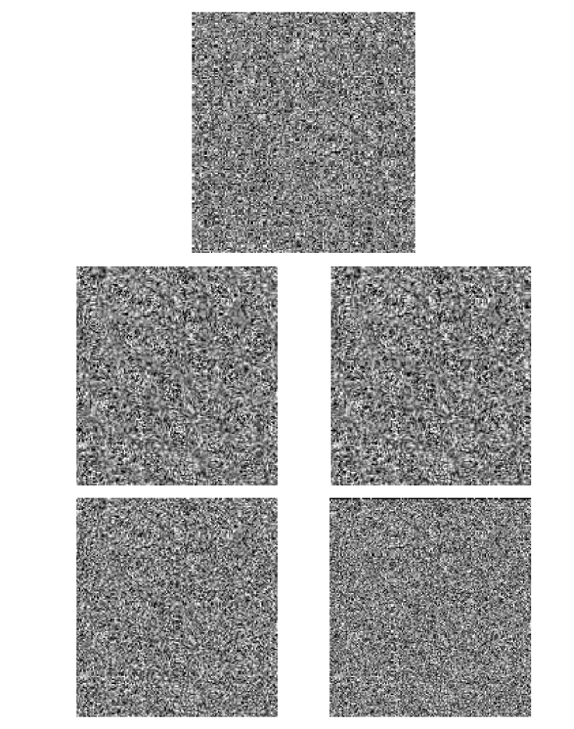
Figure 1: Results from “drizzling” white noise simulations with different interpolation kernels. On the very top at the center is shown the white noise simulation before drizzling. The central two images have been drizzled with the Bilinear (left) and Gaussian (right) kernels. The lower images have beens drizzled with the Lanczos3 (left) and Nearest (right) kernels.

Sample images for the white noise simulations are shown in Fig. 1. It is apparent that both the Bilinear and Gaussian images show visible patterns of correlation. The Nearest and Lanczos3 kernels introduce less correlation. The Nearest interpolation leaves a large number of zero (uninterpolated) pixels in the output image and does not preserve relative astrometry at the pixel scale. This is because no real interpolation is done in this case; the input pixel value is simply assigned to the nearest output pixel.

To quantify the bias arising from the interpolation, we have calculated power spectra for the simulated images. For the white noise simulation, the original image has, as expected, a flat power spectrum. However, once the drizzling has been applied, both low and high wavenumbers are contaminated by the pixel correlations introduced by the interpolation kernels. We show in Fig. 2 our results for the four different kernels. In all cases, the original power spectrum is shown as a dashed line while the power spectrum of the drizzled image is shown as the continuous line. For comparison, Fig. 3 shows the difference between the power spectra measured in the original and drizzled images.

As Fig. 2 – 3 reveal, the Bilinear and Gaussian interpolations introduce artificial pixel correlation on all scales, making it impossible to use these kernels for accurate SBF measurements. The Lanczos3 kernel depresses the power spectrum at high wavenumber (small pixel scales). The Nearest kernel does not bias in any significant way the image power spectrum, which remains flat (constant with k), even if the power spectrum is systematically lower than the original. From the noise simulations, both of the latter kernels can be used for SBF measurements in the k range in which the power spectrum remains flat ( i.e. provided the smallest pixel scales are not used when fitting the power spectrum with the Lanczos3 interpolation). From the white noise simulations drizzled with the Lanczos3 kernel, we have measured the pixel scale range in which the power spectrum is flat to within 3 $\sigma$. This is true for scales between 3 and 20 pixels, corresponding to fractional wavenumbers in the range 0.05 $\leq k\leq$ 0.33. On smaller pixel scales, the original white noise power spectrum is significantly depressed by the noise correlation.

3.2 Results from the galaxy simulations

The galaxy simulations have been performed following the method described in Mei et al. (2001b). With the galaxy magnitude and effective radius specified, the surface brightness at each pixel is calculated using a de Vaucouleurs (1948) profile and Bruzual & Charlot (2003) stellar population models corresponding to solar metallicity and an age of 12 Gyr. The results are not sensitive to the use of the de Vaucouleurs profile, since the SBF measurements are done on the galaxy model-subtracted images. The isophotal model used for the galaxy subtraction does not assume the de Vaucouleurs form (see § 2.2). Just as in real data, mismatches between the simulated galaxy images and isophotal models will produce large-scale spatial signatures in the power spectra that do not affect our fitting scales. Similarly, the precise age and metallicity of the stellar population model is not important, except insofar as they precisely specify the SBF magnitude for the simulations.

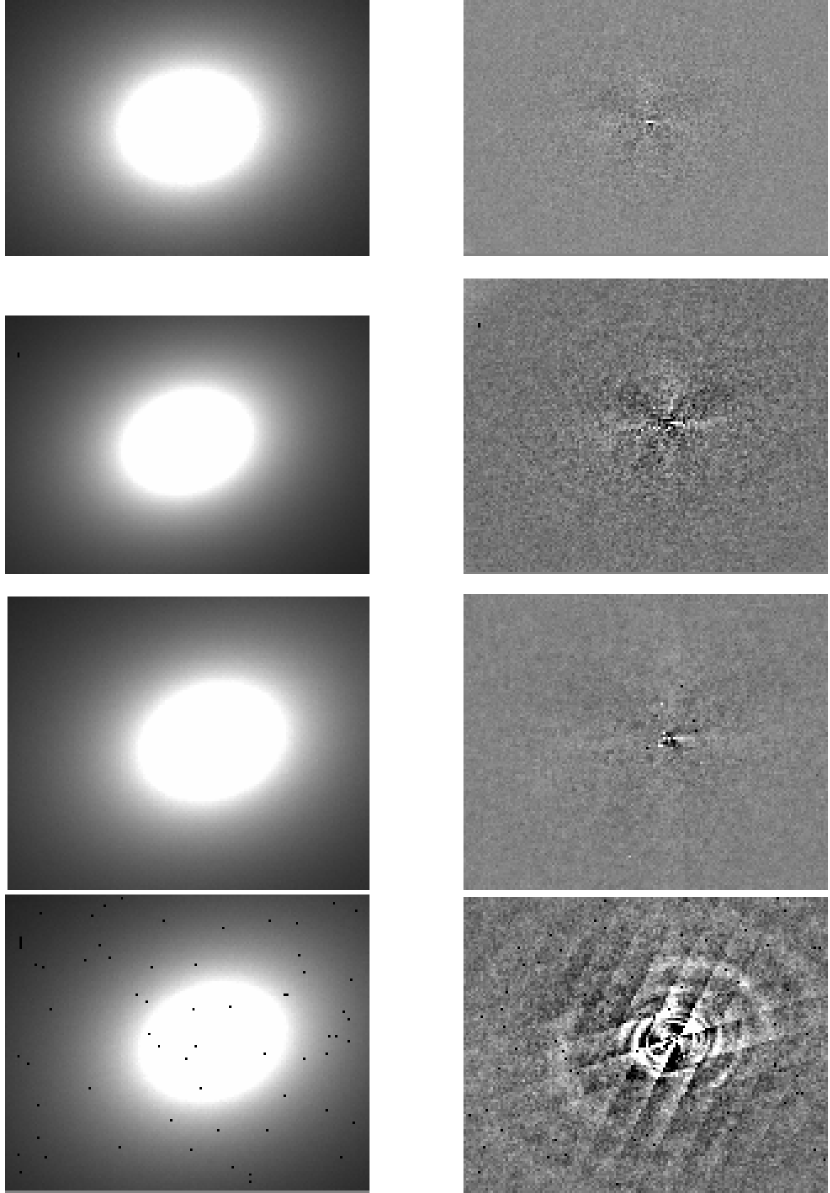
Figure 4: Results from galaxy simulations with different interpolation kernels. On the very top is shown a simulation (before drizzling) for a galaxy ($\approx 30~{}\arcsec\times 20~{}\arcsec$) with $M_{B}=-22$ (left), and the residual after subtracting a smooth galaxy model (right). The residuals show fluctuations from Poissonian noise, read out noise and the PSF-convolved Poissonian stellar fluctuations. In the center images, the same for the same galaxy image drizzled with a Gaussian and a Lancoz3 filter. In the bottom, the same, drizzled with a Nearest filter.

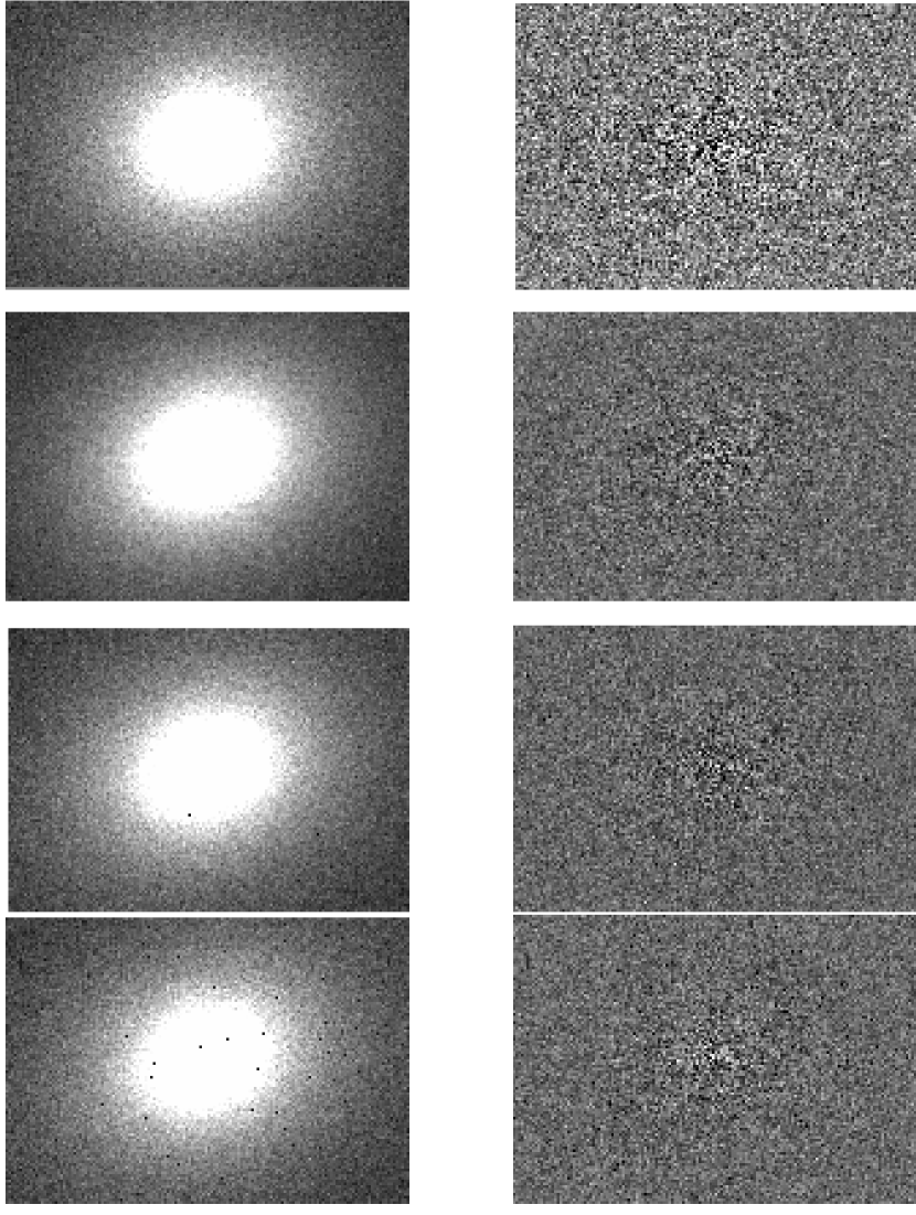
Figure 5: Results from galaxy simulations with different interpolation kernels. the same than Fig. 4, for a galaxy ($\approx 30~{}\arcsec\times 20~{}\arcsec$) with $M_{B}=-17$.

To each pixel in the simulated images, we add a Poisson variance calculated from the number of stars contributing to the pixel, Poissonian noise from the galaxy and the sky (22 mag arcesc^-2), and a read noise of 7 $e^{-}$. The images are then convolved with the PSF and drizzled using three different interpolation kernels: Gaussian, Lancsoz3 and Nearest. Since the results from the white noise simulations show that the Gaussian and Bilinear kernels introduce similar strong pixel correlations, we use only the Gaussian to quantify this effect. Moreover, in the larger context of our survey, this kernel allows a more faithful reconstruction of the galaxy centers. Galaxy simulation images are shown in Fig. 4 and Fig. 5. The left panels show the simulated galaxies and the right panels show the residuals following subtraction of smooth isophotal models. As for the white noise simulations, the Gaussian interpolation shows visible patterns in all the residuals. The Nearest interpolation shows visible residual patterns in the centers of the galaxy simulations where the intensity profile is steepest, especially for the brighter galaxy.

To quantify the effect of the interpolation on the SBF measurements, we have simulated 100 galaxies for an assumed Virgo distance of 16 Mpc, and for three galaxy magnitudes corresponding to: 1) the brightest galaxy in our sample ($M_{B}=-$22 mag); 2) the faintest galaxy ($M_{B}=-$15 mag); and 3) an intermediate galaxy ($M_{B}=-$17 mag). The $B-V$ (Vega) color from Bruzual & Charlot (2003) models is 0.97 mag, and the $V-F850LP$ (AB) color is 0.9 mag. Each of these simulations has been drizzled with the three different kernels. We then applied the SBF reduction procedure, as described above, to the simulated galaxy images to obtain SBF magnitudes, and then distances from the input SBF absolute magnitude ($\overline{M}_{F850LP}=-1.42$ from the Bruzual & Charlot stellar population model).

Histograms of the resulting SBF distances for individual annuli of the 100 galaxy image realizations are shown in Fig. 6 and summarized in Table 1. SBF magnitudes and distances are shown when the fit is performed in two different ranges: (1) between 3 to 20 pixels, and (2) between 0 to 20 pixels, i.e., out to the maximum wavenumber. The fit was not extended beyond 20 pixels because, in the real data, larger scales will be biased by the subtraction of the large–scale residuals (see § 2.2).

The Gaussian filter introduces a bias in SBF distance measurements of 6 to 20%, compared to a bias of 0.1 to 4% for the Lancsoz3 kernel. The Nearest filter tends to underestimate the distance in the innermost annuli of bright galaxies. As seen in Fig. 6, when the Nearest filter is used, the distance histogram of the brightest galaxy shows a bimodal distribution, with peaks at $\approx 11$ Mpc and $\approx 15$ Mpc, corresponding to the innermost and outermost annuli, respectively. This causes a bias of 20% on the total SBF distance of bright galaxies. For fainter galaxies, the biases due to this filter are between 1 and 2 %. However, contrary to expectations from the white noise simulations, when the Lanczos3 filter is used, galaxy distances do not significantly improve if we use a maximum wavenumber corresponding to 3 pixels. This is because of the reduced leverage for determining the $P_{1}$ value in equation (1).

We have chosen to use the Lanczos3 kernel for our final SBF analysis to insure a homogeneous data treatment between faint and bright galaxies, and because it preserves astrometric fidelity. This has the further advantage that the same images can be used for fitting globular cluster structural parameters. However, since the Lanczos3 kernel is not well adapted to isophotal analysis (e.g., negative pixel values occur near saturated or repaired pixels), we have produced a second set of images with a Gaussian kernel, used in the isophotal analysis of the program galaxies. As a visual comparison of the effects on real data, the top panel of Fig. 7 shows a corner of the M87 image drizzled with the Gaussian (left) and the Lanczos3 (right) kernel. The lower panel compares the respective weight images for the two kernels as derived from the drizzle interpolation (see Paper II).

Fig. 8 shows simulated galaxy power spectra in an annulus with inner and outer radius of, respectively, $\approx 1\arcsec$ and $\approx 6\arcsec$. On the left, the spectrum of a galaxy with an absolute $B$-band magnitude of $-$22 mag is shown before (top) and after (bottom) drizzling; on the right, the same comparison is given for a galaxy with absolute $B$-band magnitude of $-$17 mag. We have fitted the power spectrum of the original image over the entire scale range and the power spectrum of the drizzled image for scales between 3 and 20 pixel. For this particular choice of annulus, the distance values between the original and drizzled simulated images agree to $4\%$, with a corresponding difference in SBF magnitudes of $\approx$0.05 mag. In Fig 9 we show NGC 4472 power spectrum for three innermost annuli with respective inner and outer radius of 1$\farcs$6 and 3$\farcs$2, 3$\farcs$2 and 6$\farcs$4, and 6$\farcs$4 and 9$\farcs$6.

4 Conclusions

We have described the SBF data reduction procedures for the ACS Virgo Cluster Survey, paying close attention to the feasibility of SBF measurements with the ACS/WFC instrument. Although the ACS images exhibit strong geometrical distortions that could bias SBF measurements, we have shown with the aid of simulated galaxy images having realistic noise properties that it is possible to measure accurate SBF distances by correcting for biases, taking care to mask contaminants (i.e., globular clusters, foreground stars and background galaxies), and using an appropriate (Lanczos3) interpolation kernel. Future papers in this series will derive a new $z$-band SBF calibration for our sample, present the final SBF distances and their uncertainties, compare the SBF and globular cluster luminosity function distances, and examine the three-dimensional structure of the Virgo cluster.

Table 1: Measurements of SBF Magnitudes and Distances from Drizzled Simulated Images.

$M_{B}$	Kernel	Pixel scale range	SBF mag.	$\sigma_{SBF}$	Dist.	$\sigma_{Dist}$	Bias
(mag)			(mag)	(mag)	(Mpc)	(Mpc)	%
$-$22	Original	0-20	29.57	0.08	15.9	0.6	0.6
	Gauss	0-20	29.46	0.08	15.0	0.6	6
	Lanczos	0-20	29.60	0.08	16.0	0.6	0.1
	Nearest	0-20	28.91	0.66	12.2	3.2	24
$-$17	Original	0-20	29.60	0.08	16.1	0.7	0.5
	Gauss	0-20	29.41	0.08	14.7	0.5	8
	Lanczos	0-20	29.62	0.09	16.2	0.6	1
	Nearest	0-20	29.61	0.10	16.1	0.8	0.7
$-$15	Original	0-20	29.61	0.15	16.2	1.1	1
	Gauss	0-20	29.04	0.16	12.4	0.9	22
	Lanczos	0-20	29.58	0.13	16.0	1.0	0.1
	Nearest	0-20	29.62	0.14	16.2	1.1	0.2
$-$22	Original	3-20	29.58	0.10	15.9	0.7	0.6
	Gauss	3-20	29.50	0.10	15.4	0.7	4
	Lanczos	3-20	29.60	0.10	16.2	0.7	1
	Nearest	3-20	28.84	0.72	11.9	3.4	26
$-$17	Original	3-20	29.61	0.10	16.1	0.7	0.8
	Gauss	3-20	29.49	0.09	15.3	0.6	5
	Lanczos	3-20	29.65	0.10	16.5	0.7	3
	Nearest	3-20	29.61	0.10	16.2	0.8	1
$-$15	Original	3-20	29.62	0.17	16.2	1.3	1
	Gauss	3-20	29.21	0.14	13.4	0.9	16
	Lanczos	3-20	29.68	0.17	16.7	1.3	4
	Nearest	3-20	29.63	0.16	16.3	1.2	2

Figure 2: Noise power spectra when different interpolation kernels are used in the image drizzling. From top to bottom, the four panels refer to the Bilinear, Gaussian, Lanczos3, and Nearest kernels. The wavenumber $k$ corresponds to the inverse of the pixel scale. The continuous lines are the spectra after drizzling, the dashed line is the power spectra of white noise before drizzling.

Figure 3: Differences between the original and drizzled noise power spectra are shown as continuous lines for the same four cases as in Fig. 2. From top to bottom, the panels refer to the Bilinear, Gaussian, Lanczos3, and Nearest kernels. The dashed line is the case where the difference is zero.

Figure 6: The histograms of the measured SBF distances are shown for the three different magnitude simulations. For each of the 100 simulations at each magnitude, SBF magnitudes and distances have been measured in four different annuli having inner and outer radii of 1$\farcs$6 and 3$\farcs$2, 3$\farcs$2 and 4$\farcs$8, 4$\farcs$8 and 6$\farcs$4, and 6$\farcs$4 and 8″. From left to right we show results for the original galaxy simulations, and, respectively, for the Gaussian, Lanczos3, and Point/Nearest drizzled images. From top to bottom the galaxy absolute B magnitude is $-$22 mag, $-$17 mag and $-$15 mag. The solid histograms correspond to results obtained with a fit on the entire scale range, the dashed ones to fits obtained in the range between 3 to 20 pixels. The dashed vertical line corresponds to the input distance of 16 Mpc.

Figure 7: Top: a $0\farcm 5{\,\times\,}0\farcm 7$ section of the M87 image is shown when the Gaussian (left) and Lanczos3 (right) drizzle interpolation kernels are used. Bottom: the full drizzle weight images obtained for these interpolations (including weight variations from rejection of pixels affected by cosmic rays and detector defects), again with the Gaussian results on the left and the Lanczos3 results are on the right.

Figure 8: Original (top) and drizzled (bottom) power spectra for the galaxy simulations when a Lanczos3 kernel is used. The results are for an annulus with inner and outer radius of respectively $\approx$1 and $\approx$6 ″. On the left, the spectrum of a galaxy with $M_{B}=-$22 mag is shown before (top) and after (bottom) drizzling; on the right, the same thing is shown for a galaxy with absolute $M_{B}=-$17 mag. The diamonds are the image power spectra, the continuous line the fit of the power spectrum P(k), the dotted line is $P_{0}\times E(k)$ and the dot-dashed line indicates the fitted $P_{1}$.

Figure 9: VCC1226 (M49, NGC 4472) power spectra for the three innermost annuli. From top to bottom, the power spectra were calculated using annuli having inner and outer radii of 1$\farcs$6 and 3$\farcs$2, 3$\farcs$2 and 6$\farcs$4, and 6$\farcs$4 and 9$\farcs$6. The diamonds are the image power spectrum, the continuous line the fit of the power spectrum P(k), the dotted line is $P_{0}\times E(k)$, and the dashed line is $P_{1}$.

References

- Ajhar et al. (2001) Ajhar E.A., Tonry, J.L., Blakeslee, J.P. et al. 2001, ApJ, 559, 584
- Ajhar et al. (1997) Ajhar E.A., Lauer, T.R., Tonry, J.L. et al., 1997, AJ, 114, 626
- (3) Blakeslee, J. P., Ajhar, E. A., Tonry, J. L., 1999a, in Post-Hipparcos Cosmic Candles, eds. A. Heck & F. Caputo (Boston: Kluwer), 181
- (4) Blakeslee, J. P., Davis, M., Tonry, J. L. et al., 1999b, ApJ, 527, L73
- Blakeslee et al. (2002) Blakeslee, J.P., Lucey, J.R., Tonry, J.L. et al. 2002, MNRAS, 330, 443
- Blakeslee et al. (2001) Blakeslee, J.P., Vazdekis, A., & Ajhar, E.A. 2001, MNRAS, 320, 193
- Bruzual & Charlot (2003) Bruzual, G. & Charlot, S. 2003, MNRAS, 344, 1000
- Buzzoni (1993) Buzzoni, A. 1993, A&A, 275, 433
- Cantiello et al. (2003) Cantiello, M., Raimondo, G., Brocato, E., & Capaccioli, M. 2003, AJ, 125, 2783
- Côté et al. (2004) Côté, P., Blakeslee, J.P., Ferrarese, L., Jordán, A., Mei, S., Merritt, D., Milosavljević, M., Peng, E.W., & West, M.J. 2004, ApJS, 153, 223 (Paper I)
- de Vaucouleurs (1948) de Vaucouleurs, G. 1948, Ann. d’Astroph., 11, 247
- Ferrarese et al. (2000) Ferrarese L., Mould, J.R., Kennicutt R.C. 2000, ApJ, 529, 745
- Ford et al. (1998) Ford, H.C. et al. 1998, Proc. SPIE, 3356, 234
- Fruchter & Hook (2002) Fruchter, A. S. & Hook, R. N. 2002, PASP, 114, 144
- Jensen et al. (1998) Jensen, J. B., Tonry, J. L., & Luppino, G. A. 1998, ApJ, 505, 111
- Jensen et al. (1999) Jensen, J.B., Tonry, J.L., Luppino, G.A., 1999, ApJ, 510, 71
- Jensen et al. (2001) Jensen, J.B. et al., 2001, ApJ, 550, 503
- Jensen et al. (2003) Jensen, J. B., Tonry, J. L., Barris, B. J., Thompson, R. I., Liu, M. C., Rieke, M. J., Ajhar, E. A., & Blakeslee, J. P. 2003, ApJ, 583, 712
- Jerjen et al. (2001) Jerjen, H., Rekola, R., Takalo, L., Coleman, M., & Valtonen, M. 2001, A&A, 380, 90
- Jerjen (2003) Jerjen, H. 2003, A&A, 398, 63
- Jerjen et al. (2004) Jerjen, H., Binggeli, B., & Barazza, F. D. 2004, AJ, 127, 771
- Jordán et al. (2004) Jordán, A., Blakeslee, J.P., Peng, E.W., Mei, S., Côté, P., Ferrarese, L., Tonry, J.L., Merritt, D., Milosavljević, M., & West, M.J. 2004, ApJS, in press (Paper II)
- Krist (2003) Krist, J. 2003, STScI Instrument Status Report ACS2003-06
- Lauer et al. (1998) Lauer T.R., Tonry, J.L., Postman, M. et al. 1998, ApJ, 499, 577
- Liu et al. (2000) Liu. M.C., Charlot, S., Graham G.R., 2000, ApJ, 543, 664
- Liu & Graham (2001) Liu, M.C. & Graham J.R. 2001, ApJL, 557, 31
- Liu et al. (2002) Liu, M. C., Graham, J. R., & Charlot, S.2002, ApJ, 564, 216
- Luppino & Tonry (1993) Luppino, G. A. & Tonry, J. L. 1993, ApJ, 410, 81
- Mei et al. (2000) Mei, S., Silva, D., & Quinn, P. J. 2000, A&A, 361, 68
- (30) Mei, S., Silva, D. R., & Quinn, P. J. 2001a, A&A, 366, 54
- (31) Mei, S., Quinn, P.J., Silva, D.R. 2001b, A&A, 371, 779
- (32) Mei, S., Kissler-Patig, M., Silva, D. R., & Quinn, P. J. 2001c, A&A, 376, 793
- Mei et al. (2003) Mei, S., Scodeggio, M., Silva, D.R, Quinn, P.J. 2003, A&A, 399, 441
- Meurer et al. (2002) Meurer, G., Lindler, D., Benitez, N., Blakeslee, J., Bouwens, R., Clampin, M., Cox, R.C. 2002, Future EUV and UV Visible Space Astrophysics Missions and Instrumentation, eds. J. C. Blades & O.H. Siegmund, Proc. SPIE, Vol. 4854, 507
- Mieske & Hilker (2003) Mieske, S. & Hilker, M. 2003, A&A, 410, 445
- Mieske et al. (2003) Mieske, S., Hilker, M., & Infante, L. 2003, A&A, 403, 43
- Pahre & Mould (1994) Pahre, M.A. & Mould J.R. 1994, ApJ, 433, 567
- Pahre et al. (1999) Pahre, M.A., Mould, J. R., Dressler, A. et al. 1999, ApJ, 515, 79
- Press et al. (1992) Press, W.H. et al. 1992, Numerical Recipes, Cambridge University Press, New York
- Sodemann & Thomsen (1995) Sodemann, M. & Thomsen, B., 1995, AJ, 110, 179
- Sodemann & Thomsen (1996) Sodemann, M. & Thomsen, B., 1996, AJ, 111, 208
- Thomsen et al. (1997) Thomsen, B., Baum, W.A., Hammergren M. et al., 1997, ApJ, 483, L37
- Tonry (1991) Tonry, J. L. 1991, ApJ, 373, L1
- Tonry & Schneider (1988) Tonry, J.L. & Schneider, D.P., 1988, AJ, 96, 807
- Tonry et al. (1990) Tonry, J.L., Ajhar, E.A., Luppino G.A. 1990, AJ, 100, 1416
- Tonry et al. (1997) Tonry, J.L., Blakeslee, J.P., Ajhar, E.A. et al. 1997, ApJ, 475, 399
- Tonry et al. (2000) Tonry, J.L., Blakeslee, J.P., Ajhar, E.A., Dressler, A. 2000, ApJ, 530, 625
- Tonry et al. (2001) Tonry, J.L., Dressler,A., Blakeslee, J.P. et al. 2001, ApJ, 546, 681
- worthey (1993) Worthey,G. 1993, ApJ, 409, 530