Gravitational Imaging of CDM Substructure

Abstract

We propose the novel method of “gravitational imaging” to detect and quantify luminous and dark-matter substructure in gravitational-lens galaxies. The method utilizes highly-magnified Einstein rings and arcs as sensitive probes of small perturbations in the lens potential (due to the presence of mass substructure), reconstructing the gravitational lens potential non-parametrically. Numerical simulations show that the implemented algorithm can reconstruct the smooth mass distribution of a typical lens galaxy – exhibiting reasonable signal-to-noise Einstein rings – as well as compact substructure with masses as low as M_sub$\sim$$10^{-3}$ M_lens, if present. “Gravitational imaging” of pure dark-matter substructure around massive galaxies can provide a new window on the standard cold-dark-matter paradigm, using very different physics than ground-based direct-detection experiments, and probe the hierarchical structure-formation model which predicts this substructure to exist in great abundance.

1 Introduction

Arcsecond-scale strong gravitational lens systems (i.e. those with multiple lensed images) provide a wealth of information about cosmology, the lensed source and the lens galaxies themselves and considerable progress has been made in all three fields in the last twenty-five years (see e.g. Kochanek, Schneider & Wambsganss 2004). However, the accuracy in many applications (e.g. measuring H₀; Refsdal 1964) is set by the poor understanding of the mass distribution of the lens potential, limiting at the same time the use of strong lenses as probes of galaxy structure (e.g. Kochanek 1991).

It is therefore critical to exploit all available information to constrain the lens potential, for example by including non-lensing data (e.g. stellar dynamics; Koopmans & Treu 2002) – and/or extract all information on the lens potential from extended lensed images. The general problem, however, is how to solve simultaneously for both the structure of the lensed source and for the structure of the lens potential (or the lens mass distribution). Information on both are entangled in the complex structure of the multiple lensed images.

A significant step forward in disentangling this information and using it to constrain the lens potential, is the use of non-parametric image reconstruction techniques in which the source brightness distribution is reconstructed on a, in some cases adaptive, grid (e.g. Kochanek et al. 1989; Wallington, Kochanek & Koo 1995; Ellithorpe, Kochanek & Hewitt 1996; Wallington, Kochanek & Narayan 1996; Warren & Dye 2003; Treu & Koopmans 2004; Wucknitz 2004; Wucknitz et al. 2004; Wayth et al. 2005; Dye & Warren 2005; Brewer & Lewis 2005). These techniques fully exploit all information contained in the lensed images. The use of smooth parameterized potential models ensures relative ease in the separation of information about the source and the potential, since the degree of flexibility in the potential models is significantly less than in the source model.

To overcome a certain lack of freedom in the parameterized potential/mass models, Saha & Williams (1997) developed a non-parametric mass reconstruction technique. Their implementation, however, only uses constraints from point-like images and the number of free parameters in the mass models often far exceeds the number of genuine constraints. The interpretation of the results must therefore be done statistically (e.g. Williams & Saha 2000). Even so, the method is powerful in exposing the range of mass models (although some might not be physical) for systems with only lensed point images.

Gravitationally lensed images, however, are strongly correlated representations of the same lensed source, whereas the effect of the lens potential on them should be highly un-correlated on small scales. This allows them to be non-parametrically separated to a very large degree.

To illustrate this point more vividly, suppose that one observes a two or four-image lens system. Any change in the source structure will show up in all multiple images. Conversely, similar structure in the lensed images most likely arises from structure in the source and not from the unlikely coincidence of nearly-identical (small-scale) perturbations in the lens potential that happen to occur exactly in front of all lensed images. Contrary, clear structure in only one, hence not all, of the lensed images is most easily explained by a localized perturbation of the lens potential near that particular image. By casting this in likelihood terms, this illustration tells us that correlated structure in the lensed images – even though not excluded to arise from small-scale perturbations in the lens potential in front of all lensed images – is most likely the result from structure in the source. Likewise, uncorrelated structure in the lensed images is most likely the result of small-scale perturbations in the lens potential. This forms the basis of a maximum-likelihood technique that allows the source and potential information encoded in the multiple lensed images, to be separated. This does not imply, however, that all degeneracies are broken (e.g. the mass-sheet degeneracy; Falco, Gorenstein, & Shapiro 1985). It does, however, allow greater freedom in the lens potential models and the possibility to reconstruct small scale potential perturbations, arising from mass-substructure, if present.

In this paper, we have developed this notion further and extensively modify the non-parametric source reconstruction algorithm – as implemented in Treu & Koopmans (2004) – to allow for a simultaneous non-parametric source and lens potential reconstruction. This integrates the idea initially suggested by Blandford et al. (2001) and more recently by Suyu & Blandford (2005), with the semi-linear inversion technique by Warren & Dye (2003) as implemented in Treu & Koopmans (2004) into a single mathematical framework. Through the two-dimensional Poisson equation, the lens potential provides a direct gravitational image of the surface density of the lens galaxy, not affected (or potentially biased) by external shear.

The technique of gravitational imaging allows dark-matter substructure in cosmologically distant lens galaxies to be detected, imaged and quantified. Flux-ratio anomalies have already hinted at its existence, either dark or luminous (e.g. Mao & Schneider 1998; Metcalf & Madau 2001; Chiba 2002; Metcalf & Zhao 2002; Dalal & Kochanek 2002; Bradač et al. 2002; Keeton 2003). If indeed these anomalies are caused by perturbations of the underlying smooth lens-galaxy potential, a direct image of the lens-galaxy mass distribution could settle many of the still open questions, such as which mass scale contributes most to flux-ratio anomalies and whether this mass is associated with the lens galaxy (Bradač et al. 2004; Mao et al. 2004; Amara et al. 2005; Metcalf 2005).

Moreover, the unequivocal detection of dark-matter substructures around lens galaxies – without any reasonable mass-to-light ratio counterpart in deep high-resolution optical images – would be a direct vindication of the basic cold-dark-matter paradigm that predicts them to exist in large numbers (Moore et al. 1999; Klypin et al. 1999). Because substructure is expected to be more prevalent at higher redshifts (e.g. Gao et al. 2004), lens galaxies are excellent probes and gravitational imaging an excellent way to test and quantify the basic assumptions of the dark-matter and the hierarchical structure formation models.

In Section 2, we derive an iterative set of linear equations that solve simultaneously for the source structure and the lens potential. We also discuss which form of regularization to use and how to determine the regularization parameters through a Maximum Likelihood analysis. In Section 3, we illustrate the method with a simulated Einstein ring. In Section 4, we draw conclusions.

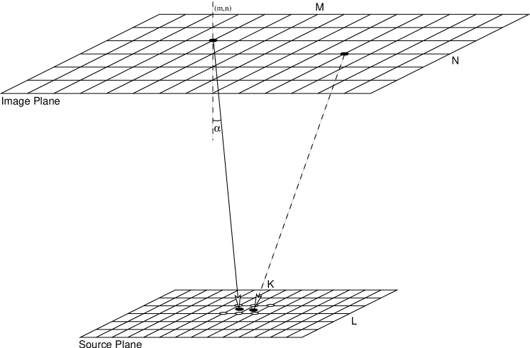
Figure 1: A schematic overview of the method of non-linear image (i.e. source) reconstruction, as implemented by Treu & Koopmans (2004) and in this paper. In the absence of blurring or averaging inside pixels, the position ($\vec{x}$) of each pixel $(m,n)$ in the image plane corresponds to a position in the source plane ($\vec{y}$), through the lens equation $\vec{y}=\vec{x}-\vec{\alpha}(\vec{x})$. The surface brightnesses at these corresponding points – conserved through lensing – are the same. Because the source brightness distribution is reconstructed on a fixed grid, the surface brightness at $\vec{y}$, i.e. $\Sigma(\vec{y})=\Sigma(\vec{x})$, is represented by a linear superposition of the surface brightnesses at the four pixels that enclose $\vec{y}$ (open circles). The weights for each of these source pixels are the bilinear interpolation weights, whose sum add to unity to conserve flux (higher-order interpolation is also possible; see Treu & Koopmans 2004). This way – because of the multiple nature of the lensed images – there can be more than one constraint on a single source pixel (depending on its size and the number of multiple images). In addition, because there are multiple solutions of four weighted brightnesses adding to the observed brightness at $\vec{x}$, regularisation is often required to ensure a relatively smooth and more physical source brightness distribution for lower signal-to-noise data (see text).

2 The Method

In this section, before we extend the non-parametric method to include a non-parametric reconstruction of the lens potential, we first discuss the non-parametric reconstruction method for only a pixelized source, but given a smooth parameterized lens-potential model.

2.1 The non-parametric source solution

The non-parametric reconstruction method of a pixelized source is shown schematically in Fig. 1. The figure illustrates how the surface brightness of each image pixel can be represented through a weighted linear superposition of the (unknown) surface brightnesses at four source pixels. Hence, one can represent this as a simple linear equation (see Koopmans & Treu 2004) and because this holds for each of the M$\times$N image pixels, one obtains a set of M$\times$N coupled linear equations. This set of equations is constrained by the M$\times$N observed surface brightnesses values (i.e. ${\vec{d}}$) and has K$\times$L free parameters (i.e. $\vec{s}$; the unknown surface brightnesses values on the source grid).

As was shown in Koopmans & Treu (2004) and also Warren & Dye (2003), the pixelized lensed image (with the lens-galaxy subtracted and blurring included) can then be expressed as the set of linear equations

$${\bf B}{\bf L}(\psi)\,\vec{s}={\vec{d}},$$ (1)

where ${\bf L}(\psi)$ and ${\bf B}$ are the lensing and (also linear) blurring operators, respectively, and $\psi$ is the lens potential which for simplicity is here also representing the set of unknown lens-potential parameters. Each row of the lensing operator (a sparse matrix) only contains the four bi-linear interpolation weights, placed at the columns that correspond to the four source pixels that enclose the associated source position (Fig. 1; see Treu & Koopmans 2004 for details).

The set of equations (1) is in general ill-posed (i.e. under-constrained and/or noisy data) and can not be solved through $\vec{s}=[{\bf B}{\bf L}(\psi)]^{-1}{\vec{d}}$. Instead, there exist well-known regularized inversion techniques that minimize the quadratic penalty function

$$G(\vec{s},\psi)=||{\bf M}\vec{s}-{\vec{d}}||_{2}^{2}+\sum_{i}\lambda_{i}||{\bf H}_{i}\vec{s}||^{2}_{2},$$ (2)

by varying $\vec{s}$ (we define ${\bf M}\equiv{\bf B}{\bf L}(\psi)$). In addition, ${\bf H}_{i}$ are regularization matrices and $\lambda_{i}$ are the corresponding regularization parameters, both of which we discuss in more detail below (see also Press et al. 1992 for a clear discussion about regularization methods). The first term in the penalty function $G(\vec{s},\psi)$ is proportional to the total $\chi^{2}$ for a given solution $\vec{s}$ and as such quantifies how well the model matches the data. The second terms can regularize the “smoothness” of the solution by adding a positive quadratic penalty term, whose argument depends linearly on the source solution, i.e. through ${\bf H}_{i}\vec{s}$, which for example could give its $n$-th order derivative. The quadratic nature of the regularization term ensures that the minimum–$G$ solution can be found by solving a linear set of equations (this is not the case for maximum-entropy or maximum-likelihood regularization terms). The quadratic nature of the regularization term dramatically reduces the time to numerically find the best source solution and ensures that the global minimum of $G$ is found (given a fixed $\psi$).

By setting the derivative $\partial G(\vec{s},\psi)/\partial\vec{s}=0$, a bit of linear algebra then leads to the required set of equations

$$\left[{\bf M}^{T}{\bf M}+\sum_{i}\lambda_{i}{\bf H}^{\rm T}_{i}{\bf H}_{i}\right]\vec{s}={\bf M}^{\rm T}{\vec{d}},$$ (3)

whose solution for $\vec{s}$ minimizes $G(\vec{s},\psi)$, by construction, for a fixed lens potential $\psi$. In an outer non-linear optimization loop (see Warren & Dye 2003) one then varies the free parameters of $\psi$ to find the global minimum of the joint penalty function, $G(\vec{s},\psi)$, resulting in an optimized non-parametric source model and an optimized set of parameters for the lens potential.

In this way, one makes full use of all information in the lensed images to constrain the parameterized potential model $\psi$, without strong assumptions about the structure of the source. However, there are several questions that arise:

(1) Does the parameterized potential model $\psi$ have enough freedom to describe the true lens potential?

(2) Which form for the regularization matrices, ${\bf H}_{i}$, should be used?

(3) What should be the values of the regularization parameters $\lambda_{i}$ in the penalty function $G$?

To (partly) address these questions, we derive in section 2.2 a new set of linear equations, whose min–$G$ solution gives the pixelized source structure and simultaneously a linear pixelized correction ($\delta\vec{\psi}$) to the initial model of the lens potential. By solving this new set of equations and correcting the potential model iteratively, one minimizes the penalty function to find a non-parametric and non-linear solution for both the source structure and the lens potential.

We choose to pixelize and solve for the lens potential, in contrast to e.g. Saha & William (2000) who solve for a pixelized mass distribution. Both are related through the two-dimensional Poisson equation. However, because all properties of the lens system can be derived solely from the local lens potential (through its zero-th, first and second order derivatives), no assumptions have to made about what happens outside the region where we have lensing information (i.e. the lensed images). On the other hand, if one chooses to use a pixelized mass distribution, one needs to make some a priori assumptions about the mass distribution outside the grid (e.g. no mass), since mass outside the grid still contributes to the lens potential inside the grid. If wrong assumptions are made, for example one assumes there is no potential arising from external shear (i.e. $\psi_{\rm sh}(\vec{x})=0$) whereas in fact there is, one can severely bias the resulting solution for the pixelized mass distribution, because the contribution from shear must then somehow be mimicked by the mass distribution inside the grid.

In the case of a pixelized potential model, however, the lens potential due to external mass (i.e. from outside the grid) would be reconstructed without a problem, just like that arising from mass inside the grid. The Poisson equation, furthermore, only gives the mass distribution inside the grid, not affected by e.g. external shear (because $\nabla^{2}\psi_{\rm sh}(\vec{x})=0$) or any mass external to the grid. The reconstructed mass distribution can therefore never be biased by assumptions about the mass distribution outside the grid. We regard the latter as a great advantage over the use of a pixelized mass distribution.

A second advantage of using the lens potential over the lens mass distribution is increased numerical speed in the optimization process. In case a mass distribution is used, the lens potential still needs to be calculated through a convolution. This is a significant numerical burden, whereas all lens properties can simply and quickly be derived from a lens potential through its $n$–th order derivatives ($n$=0, 1 or 2).

Despite these advantages, the use of a pixelized mass distribution provides a means of retaining a positive surface density. However, when we regularise the potential model by minimizing the norm of its $n$-th order derivative, we regularize the mass density in its ($n$$-$2)–th order derivative (because of the second order derivative in the Poisson equation). Because we start with a smooth positive-density mass model and only make a relative small potential correction, the regularization can thus ensure that the surface density of the mass model remains positive, even though we reconstruct the lens potential (see also §2.3.1).

The second and third questions, stated above, are of more general interest in many similar (image-reconstruction) problems and are addressed in sections 2.3 and 2.4, within the context of the problem at hand.

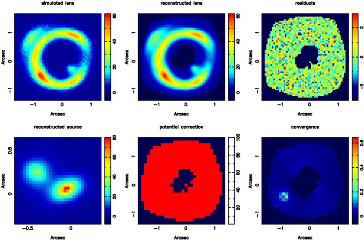
Figure 2: Reconstruction of the source and lens-potential correction using the true mass model. Top row: A simulated Einstein-Ring lens system (see text) (left). The best reconstruction (middle) and residuals (right). Bottom row: The reconstructed source (left). The correction to the lens potential, set to zero for this model (middle), and the total convergence minus a best-fit SIE mass model (right). The shape of the reconstructed region is determined by the projection of the rectangular source plane on to the image plane. This results in a hole in the center of the reconstruction, since the source plane (in this case) maps on to a closed annulus. Outside the annulus, image-plane pixels map outside the source-plan grid.

2.2 The non-parametric source and potential solutions

To find a linear correction to, say, a parameterized potential model (e.g. found as described in § 2.1) we assume that the potential $\psi$ is also pixelized (i.e. ${\vec{\psi}}$ are the pixel values). We note that the number and size of the pixels for the potential grid need not be the same as for the image grid.

Given the previously-found best-fit source model $\vec{s}_{\rm p}$ and potential-model ${\vec{\psi}}_{\rm p}$, one can then subtract the best-fit lens model from the data and obtain a residual image

$$\delta\vec{d}={\vec{d}}-{\bf M}({\vec{\psi}}_{\rm p})\,\vec{s}_{\rm p}.$$ (4)

If $||\delta\vec{d}/\sigma_{d}||^{2}\gg(MN)$, where $\sigma_{d}^{2}$ is variance per image pixel, either the source or the potential model is not correct, or both. We can then assume that a potential correction, ${\delta\vec{\psi}}$, exists for which to first order

$${\vec{d}}-{\bf M}({\vec{\psi}}_{\rm p}+{\delta\vec{\psi}})\,\vec{s}_{\rm p}\rightarrow\vec{0}.$$ (5)

It is our task to find ${\delta\vec{\psi}}$ and with it correct the previously best-fit potential model ${\vec{\psi}}_{\rm p}+{\delta\vec{\psi}}\rightarrow{\vec{\psi}}$. With the previous source solution, $\vec{s}_{\rm p}$, this can to first order also be written as new set of linear equations (Appendix A)

$$\delta\vec{d}=-{\bf B}{\bf D}_{s}(\vec{s}_{\rm p}){\bf D}_{\psi}{\delta\vec{\psi}},$$ (6)

where ${\bf D}_{s}(\vec{s}_{\rm p})$ is a sparse matrix whose entries depend on the gradient of the previously-best source model and ${\bf D}_{\psi}$ is a matrix that determines the gradient of ${\delta\vec{\psi}}$. Note also that the image blurring is accounted for (see Koopmans & Treu 2004). Combining equation (6) with equation (4), one finds

$${\bf B}\left[{\bf L}({\vec{\psi}}_{\rm p})\vec{s}-{\bf D}_{s}(\vec{s}_{\rm p}){\bf D}_{\psi}{\delta\vec{\psi}}\right]={\vec{d}}$$ (7)

If we further introduce the block matrix

$${\bf{L}_{\rm c}({\vec{\psi}}_{\rm p},{\vec{s}}_{\rm p})}\equiv\left(\begin{array}[]{ccc}{\bf L}({\vec{\psi}}_{\rm p})\mid-{\bf D}_{s}(\vec{s}_{\rm p}){\bf D}_{\psi}\end{array}\right)$$ (8)

and the block vector

$$\vec{r}\equiv\left(\begin{array}[]{c}\vec{s}\\ {\delta\vec{\psi}}\end{array}\right),$$ (9)

the final linear set of equations becomes

$${\bf B}{\bf{L}_{\rm c}({\vec{\psi}}_{\rm p},{\vec{s}}_{\rm p})}\,\vec{r}\equiv{\bf{M}_{\rm c}}\,\vec{r}={\vec{d}}$$ (10)

The structure of this equation is the same as that of equation 1 and can thus be solved as before. We note that because the first term of equation 7 depends only on ${\vec{\psi}}_{\rm p}$ and $\vec{s}$, whereas the second terms depends only on ${\delta\vec{\psi}}$ and $\vec{s}_{\rm p}$, they are decoupled sets of equations that could be solved independently.

How can the correction in equation (6) be interpreted? This is most easily seen when writing the equation in its continuous form $\delta d(\vec{x})=-\vec{\nabla}_{y}s(\vec{y})\cdot\vec{\nabla}_{x}\delta\psi(\vec{x})$ as shown in Appendix A. Because $\vec{y}=\vec{x}-\vec{\nabla}\psi$ and $\delta\vec{y}=-\vec{\nabla}\delta\psi$, what equation (6) tells us is that to first order the deviation of $\delta d(\vec{x})$ from zero can be compensated exactly by Taylor expanding $s(\vec{y})$ to first order around $\vec{y}$ and then changing the deflection angle slightly by $\delta\vec{y}$ to point to that part of the source, close to $\vec{y}$, that has the same surface brightness as that seen at the image position $\vec{x}$. The trick is to find the solution $\delta\psi(\vec{x})$ such that $\delta d(\vec{x})\rightarrow 0$ for all $\vec{x}$. This is what has been done above, by linearizing the equations and writing the result in matrix/vector notation.

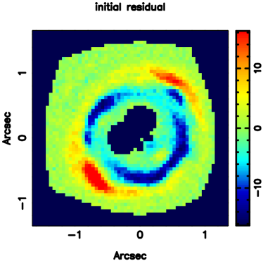
Figure 3: The residuals of the data minus the “best” reconstruction, assuming a SIE mass model fit to the image centroids only. Note the difference with the final residuals in Figure 4.

2.3 The Regularization Matrix

Because $\vec{s}$ and ${\delta\vec{\psi}}$ are independent, they require their own regularization parameters. Consequently, the regularization matrix needs to be modified somewhat:

$${\bf R}\equiv\left(\begin{array}[]{cc}\sum_{j}\lambda_{s,j}{\bf H}^{\rm T}_{s,j}{\bf H}_{s,j}&0\\ 0&\sum_{j}\lambda_{\delta\psi,j}{\bf H}^{\rm T}_{\delta\psi,j}{\bf H}_{\delta\psi,j}\end{array}\right).$$ (11)

The set of equations, whose solution minimizes the penalty function, then becomes

$$\left({\bf{M}^{T}_{\rm c}}{\bf{M}_{\rm c}}+{\bf R}\right)\vec{r}={\bf{M}^{T}_{\rm c}}{\vec{d}}.$$ (12)

Hence, by iteratively solving equation (12) and correcting the lens potential at each iteration, one finds the source and potential structure that minimize $G$ without strong assumptions about either. This equation is the equivalent of equation (3).

2.3.1 Regularizing with higher-order derivative operators

The form of the regularization matrices is not a-priori determined. But since “smoothness” is often a criterion for how well the reconstruction has been done, most often derivative operators are used for the regularization matrices (see Press et al. 1992 for some examples); the zeroth order derivative being the identity matrix. Their mathematical structure is also the best understood of all forms (see Neumaier 1998 for a complete analysis).

We use different derivative-orders for the source and the potential regularization. We find that zeroth order derivative, ${\bf H}={\bf I}$, gives poor source reconstruction in the majority of cases, especially if the signal-to-noise ratio of the data is low (see Treu & Koopmans 2004 for some discussion) and worse for the potential reconstruction, that requires smoothness in very high order (see below). One solution is to resort to multi-scale pixels in the source plane (Dye & Warren 2005), which is an implicit form of adaptive regularization. But its hard to require smoothness (or continuity) in the solutions and their derivatives.

For this reason, a much better choice of regularization for single-scale pixels, is the use of higher-order derivative operators. In those cases neighboring pixels are “connected”, resulting in considerably improved solutions.

It is found that regularization with a single second-order derivative operator (i.e. minimizing curvature) is often sufficient to reconstruct the source. To require the convergence (i.e. surface density) of the lens to be smooth, the potential regularization requires at least a single fourth-order derivative operator. Since $\delta\kappa/\kappa\ll 1$ and $\delta\kappa$ is smooth for any good starting model, one ensures in general positive convergence solutions.

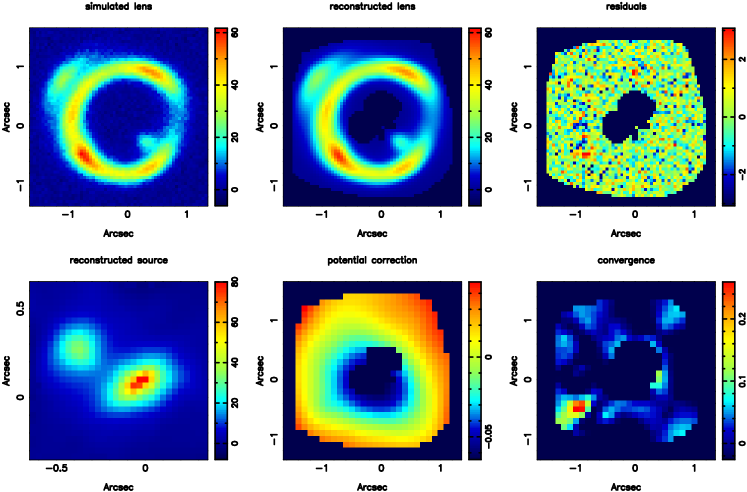
Figure 4: Reconstruction of the source and lens-potential correction using a best-fit single SIE mass model as starting model. Top row: A simulated Einstein-Ring lens system (see text) (left). The best reconstruction (middle) and residual images (right). Bottom row: The reconstructed source (left). The correction to the lens potential (middle) and the lens convergence minus a best-fit SIE mass model (right).

2.4 The Regularization-Parameter Values

Having chosen appropriate regularization matrices, the next question is which level of regularization is appropriate.

(i) The “subjective” way of choosing their numerical values is through a careful analysis of simulated lens systems that closely resemble the real lens system. The regularization-parameters values are then chosen such that the input models are best recovered. Because the real system resembles the simulated system, one assumes that the obtained value for the regularization parameter also gives an unbiased reconstruction of the source and potential of the real system.

(ii) The “objective” way is to have the data itself determine the regularization-parameter values. Intuitively, one might think that the probability distribution of pixel values of the difference between the observed system and the model should be that of “noise” with zero mean and show no residual structures. How can in that case, the numerical values of $\lambda_{s/\delta\psi,j}$ be determined?

As often is the case in CCD images, if the noise is approximately Gaussian distributed, this can be expressed for a fixed $\psi$, as the maximization of the likelihood

$${\cal L}=\frac{1}{(2\pi)^{NM/2}\sqrt{{\rm det}(\sigma_{d}^{2}{\rm{\bf I}})}}\exp\left[-({\vec{d}}-{\bf M}\tilde{s})^{\rm T}({\vec{d}}-{\bf M}\tilde{s})/(2\,{\sigma_{d}^{2}})\right],$$ (13)

with $\sigma_{d}^{2}$ being the variance of the image pixels, assuming that the covariance between different pixels is zero, and $\tilde{s}$ being the solution from equation (3). What this equation means is that the maximum-likelihood value of $\lambda$ should, as closely as possible, result in a zero-mean Gaussian residual image $\delta{\vec{d}}$. As an illustration, if $\lambda$ (encoded in $\tilde{s}$) is too small, the model will fit the noise, resulting in a “flat” residual distribution function (i.e. the lowest noise values becomes part of the model and consequently don’t show up in the residual image). On the other hand, if $\lambda$ is too large, the residual image will show coherent non-Gaussian structures that could not be fitted because of the over-regularization. In both cases, the residuals deviate from Gaussian, resulting in a low likelihood for the model.

Using the estimate of $\tilde{s}$ from equation (3), it has been shown shown by Wahba (1985; see also Neumaier 1998) that the Maximum Likelihood value of the regularization parameter for the source can then be found by maximizing the likelihood function,

$${\cal L}=\log(||{\vec{d}}||_{2}^{2}-||\vec{u}||_{2}^{2})-\log(\lambda)+\frac{2}{n}\log{\rm det}({\bf C}),$$ (14)

where ${\bf C}{\bf C}^{T}={\bf M}^{T}{\bf M}+\lambda\,{\bf H}^{\rm T}{\bf H}$ is obtained through a Cholesky decomposition, $\vec{u}$ is found by solving ${\bf C}\vec{u}={\bf M}^{T}{\vec{d}}$ and $n=KL$ is the number of source pixels. The result is independent from the variance ${\sigma_{d}^{2}}$, which therefore does not have to be explicitly known a priori. The ML solution of the source is obtained by solving ${\bf C}^{T}\vec{s}=\vec{u}$. Hence equation 14 is the equivalent of equation 13, but now explicitly expressed with $\lambda$ and in such a way that it is easy to solve numerically through a Cholesky decomposition that also gives the solution for $\vec{s}$ without much additional effort (i.e. through a fast back-substitution, because ${\bf C}$ is a diagonal matrix).

Since we solve iteratively for the lens potential, it is found that the value of the regularization for the potential is almost irrelevant if chosen large enough (it just takes longer to converge for stronger regularization). Furthermore, since the solutions of $\vec{s}$ and ${\vec{\psi}}$ are decoupled in the set of linear equations, as we discussed above, determining the value of $\lambda$ for the source separately from the potential is mathematically correct.

3 Gravitational Imaging of Galaxy (Sub)structure

Having introduced the methodology above, we refer to appendix B for an outline an iterative algorithm of the method. Although it is not necessarily the only or most optimal implementation, it is relatively easy to implement and robust. To test the algorithm, we performed a simulation of an artificial Einstein-ring and subsequently reconstruct the source and lens potential.

In §3.1, we first describe the simulated lens system. The source is chosen to be a double structure, consisting of two elliptical galaxies. Similarly, the lens is a smooth elliptical mass distribution plus an additional low-mass substructure. The aim of this simulation is to show that the method/algorithm is capable of reconstructing both the source structure and the small-scale mass distribution (i.e. the mass substructure) on the lens galaxy.

3.1 Artificial Einstein-ring Lens System

The components of the lens-system are:

(1) Lens Mass Model: The lens mass model consists of a single SIE lens (Kormann et al. 1994) with a lens strength of $b$=$0\aas@@fstack{\prime\prime}9$, a position angle (PA) of $\theta$=$45^{\circ}$, an axial ratio of $f$=$(b/a)_{\kappa}$=$0.8$ and centered at $(0\aas@@fstack{\prime\prime}0,0\aas@@fstack{\prime\prime}0)$. The mass model also includes a dwarf-satellite represented by a SIS with $b=0\aas@@fstack{\prime\prime}045$ at $(-0\aas@@fstack{\prime\prime}9,-0\aas@@fstack{\prime\prime}4)$ (placed on the Einstein ring). Since typical lens galaxies with these image separations have $M_{\rm E}$$\sim$$10^{11}$ M_⊙ inside their Einstein radius, this particular substructure has a mass of $M_{\rm E}$$\sim$$10^{8}$ M_⊙.

(2) Source Brightness Model: To show that complexity in the source and lens-potential models can be disentangled, the source consist of two components: (1) A subcomponent with an elliptical exponential brightness profile with $0.1$–arcsec scale-length, a central surface brightness of 100 arcsec^-2 (arbitrary units), an axial ratio of 0.64, a PA=113^∘ and centered at $(-0\aas@@fstack{\prime\prime}05,0\aas@@fstack{\prime\prime}05)$. (2) A subcomponent with an exponential brightness profile of $0.1$–arcsec scale-length, a central surface brightness of 50 arcsec^-2, centered at $(-0\aas@@fstack{\prime\prime}40,0\aas@@fstack{\prime\prime}25)$. The source is pixelized on a 1$\aas@@fstack{\prime\prime}$0$\times$1$\aas@@fstack{\prime\prime}$0 grid of $30\times 30$ pixels.

(3) Simulated Lensed Images: The lensed image is calculated on a 3^′′$\times$3^′′ grid of 60$\times$60 pixels and blurred by an artificial HST–ACS F814W PSF. Gaussian noise with $\sigma=1$ is added to the resulting blurred image. The simulated system and reconstructed source model are shown Fig.2.

3.2 The Non-Parametric Source and Lens-Potential Reconstruction

We perform two reconstructions. The first is a test-run and reconstructs only the source structure, assuming that we have perfect knowledge of the true lens mass model. This is not a realistic situation, but it shows that the method properly recovers the input source model without significant residuals. The potential grid is defined on a 3^′′$\times$3^′′ grid of 30$\times$30 pixels, sufficient to capture (sub)structure in the lens potential. The result is shown in Figure 1. The input source and Einstein ring are nicely reconstructed and the residuals are not significant ($\chi^{2}/{\rm NDF}$=0.96).

The second run should represent a more realistic situation. As would be done with an observed lens system, we find the source and lens-potential model in a number of distinct steps: (1) First, we fit a single SIE mass model to the four image centroids; the resulting best-fit parameters are $b$=$0\aas@@fstack{\prime\prime}85$, a PA of $\theta$=$47^{\circ}$, an axial ratio of $f$=$(b/a)_{\kappa}$=$0.84$). The residuals have $\chi^{2}$/NDF=29.4, hence the model is dramatically far from the true mass model (see Figure 3). Although statistically a very poor model, we can use this as the initial starting model for the non-parametric reconstruction. (2) We non-parametrically reconstruct the source and the lens-potential correction, with a regularization parameter for the source ($\lambda_{\rm s}$=3.0; which is clearly too large) and the potential ($\lambda_{\delta\psi}=10^{9}$), respectively. We lower the regularization parameters of the potential by 0.1 of its previous value each iteration and iterate $\sim$60 times, until convergence ($\sim$30 minutes on a 3–GHz laptop). (3) Using this solution, which is an extreme improvement ($\chi^{2}$/NDF=1.19), we use the ML technique (Section 2.4) to determine the value of the source regularization parameter, $\lambda^{\rm ML}_{\rm s}=0.4$. (4) We rerun the simulation with the new value of the regularization parameter. We note that the precise value of $\lambda_{\rm s}$ in the second run is nearly independent from its value in the first run, justifying this approach.

The best model has $\chi^{2}$/NDF=1.05 and is shown in Fig. 4, a dramatic improvement over the best-fit single SIE mass model. We subtract a best-fit single SIE mass model (fitted to the total convergence; see lower-right panel) to highlight any substructure of the lens. The small mass-perturbation is indeed recovered near the correct position and with good dynamic range, compared with the residuals in the convergence field. We note that regularization smooths the structure of the small mass component, which is unavoidable. However, within a $0\aas@@fstack{\prime\prime}7\times 0\aas@@fstack{\prime\prime}7$ aperture centered on the substructure (approximately the region of positive convergence after the smooth model was subtracted), we recover the original mass of the substructure to within 12%. This shows that one can not only detect, but also quantify its mass.

We note that the final solution has positive convergence everywhere inside the grid. In Figures 2 and 4 only the convergence is show after subtracting a smooth SIE model, hence the residual from this could be negative (as opposed to the total convergence).

Although we only presented a single simulation in this paper, we find that the algorithm can also reconstruct both the source and the lens potential in more complex and lower S/N cases. A more thorough analysis of the method, its errors and degeneracies, however, is planned. It should include blind tests on N-body simulated lens systems and the use more realistic source structures.

4 Conclusions

A new non-parametric source and lens-potential reconstruction method has been presented and implemented. The method has been used to gravitational image substructure in an artificial (but reasonably realistic) lens system, recovering the position and enclosed mass of the substructure, as well as the structure of the lensed source. We also conclude that the method can disentangle structure in the source and lens potential, without strong assumptions about either.

Further improvements, however, are still required: (i) Determination of the full covariance matrix to determine the errors and correlations between the source brightness pixels and potential-correction pixels. (ii) The use of a Markov–Chain Monte–Carlo technique to determine the correct (non-linear) errors for each of the source and potential pixel values. This provides a way of estimating errors in real lens systems where Monte-Carlo simulations are not feasible. (iii) Testing multi-scale pixel schemes (Dye & Warren 2005) against single-scale pixel schemes with adaptive regularization. Due to severe computational limits, however, we have not yet implemented these.

Having demonstrated its feasibility, gravitational imaging can serve as a new tool to discovery and quantify the level and evolution of the (dark-matter) substructure in the halos around galaxies at cosmological distances. Through it, the cold-dark-matter paradigm and the hierarchical structure formation models can be tested.

Appendix A Linear correction of the lens potential

Given the best-fit solution to equation 3 for both the potential $\psi$ and source $\vec{s}$, one can determine the residual vector

$$\delta\vec{d}={\vec{d}}-{\bf M}(\psi)\,\vec{s}.$$ (15)

Hence one subtracts the best lensed source model (blurred with the PSF) from the data. Suppose further that any significant residuals are due to deviations of $\psi$ from the true potential (this can’t strictly be true, because $\vec{s}$ must also be slightly wrong if $\psi$ is slightly wrong). The question arises which correction to the potential, $\delta\psi$, we have to apply such that, after the correction, the residual vector becomes

$$\delta\vec{d}={\vec{d}}-{\bf M}(\psi+\delta\psi)\,\vec{s}\approx\vec{0}.$$ (16)

This can be derived as follows, for now regarding the image, the source and the potential as scalar functions $d(\vec{x})$, $s(\vec{x})$ and $\psi(\vec{x})$, respectively, and neglecting the PSF. From a simple linear expansion of the lens equation $\vec{y}=\vec{x}-\vec{\nabla}_{x}\psi(\vec{x})$ (e.g. Schneider et al. 1992) it then follows that

$$\vec{y}+\delta\vec{y}=\vec{x}-\vec{\nabla}_{x}(\psi(\vec{x})+\delta\psi(\vec{x}))$$ (17)

or simply (for a fixed position $\vec{x}$)

$$\delta\vec{y}=-\vec{\nabla}_{x}\delta\psi(\vec{x}).$$ (18)

Hence a change in the source position is related to a change in the gradient of the lens potential. By adding a correction, $\delta\psi(\vec{x})$, to the lens potential we can “move around” rays of light hitting the source plane. Thus, our task is to find that correction to the potential $\delta\psi(\vec{x})$, that obeys the following relation: $s(\vec{y}+\delta\vec{y})-s(\vec{y})=\delta d(\vec{x})$ [i.e. the brightness of the lensed image at $\vec{x}$ equals the brightness of the source at position $\vec{x}-\vec{\nabla}_{x}(\psi(\vec{x})+\delta\psi(\vec{x}))$]. The residual field is then to first order

$$\delta d(\vec{x})=s(\vec{y}+\delta\vec{y})-s(\vec{y})\approx\vec{\nabla}_{y}s(\vec{y})\cdot\delta\vec{y}.$$ (19)

Combining equations (A4) and (A5), one finds

$$\delta d(\vec{x})\approx-\vec{\nabla}_{y}s(\vec{y})\cdot\vec{\nabla}_{x}\delta\psi(\vec{x}),$$ (20)

to first order. This has previously been derived by Blandford et al. (2001). The next step is now to derive the equivalent equation for $\delta\vec{d}$ in equation 4.

First, we assume that the potential grid has $P\times Q$ pixels ($P$ columns and $Q$ rows) with $p=1\dots P$ and $q=1\dots Q$. In addition, the potential values are $\psi_{h}$ with $h=p+(q-1)P$ and $h=1\dots PQ$. The source and data-grids are defined and described in Treu & Koopmans (2004).

We can now derive equation 4. First, we define

$${\bf D}_{s}(\vec{s}_{\rm p})=\left(\begin{array}[]{cccccc}\dots&\\ &\frac{\partial s_{h}}{\partial y_{1}}&\frac{\partial s_{h}}{\partial y_{2}}\\ &&&\frac{\partial s_{h+1}}{\partial y_{1}}&\frac{\partial s_{h+1}}{\partial y_{2}}\\ &&&&&\dots\\ \end{array}\right),$$ (21)

where the entries indicate the gradient of source brightness distribution in the $y_{1}$ and $y_{2}$ directions in the source plane. The entries are evaluated at the potential-grid positions $\vec{y}_{h}=\vec{x}_{h}-\vec{\nabla}\psi(\vec{x}_{h})$ (the potential grid can be different from the data grid). In addition, if

$${\bf D}_{\psi}{\delta\vec{\psi}}=\left(\begin{array}[]{cccccc}\dots&\\ &\frac{\partial\delta\psi_{h}}{\partial x_{1}}\\ &\frac{\partial\delta\psi_{h}}{\partial x_{2}}\\ &&\frac{\partial\delta\psi_{h+1}}{\partial x_{1}}\\ &&\frac{\partial\delta\psi_{h+1}}{\partial x_{2}}\\ &&&&&\dots\\ \end{array}\right),$$ (22)

It is then easy to see that $\delta\vec{d}=-{\bf D}_{s}(\vec{s}_{\rm p}){\bf D}_{\psi}{\delta\vec{\psi}}$ (not blurred) gives a vector whose entries are given by Eq. 20. The PSF smearing is simply included by multiplying with the blurring operator ${\bf B}$. The gradients can be evaluted through finite-differencing schemes. Higher-order schemes will ensure continuity in the derivatives of the source brightness distribution and potentials.

Appendix B The Algorithm and Implementation

By solving equation 12, adding the correction ${\delta\vec{\psi}}$ to the previously best potential model and iterating this procedure, both the potential model ${\vec{\psi}}$ and source model $\vec{s}$ should converge to a solution that minimizes the penalty function $G(\vec{s},\psi)$. We find the following algorithm to work very well, typically converging in $<$ 100 iterations:

$$1. {\tt i=0},~{}~{}\vec{s}_{i}=\vec{0},~{}~{}\Delta\vec{\psi}_{i}=\vec{0}$$

$${\tt\vec{\psi}_{0}=initial~{}model}$$

$$2. {\tt Determine~{}D_{s}(\vec{s}_{i}),L_{c}(\vec{\psi}_{0}+\Delta\vec{\psi}_{i})}$$

$$3. {\tt Solve~{}\left(M_{c}^{T}\,M_{c}+R\right)\vec{r}=M_{c}^{T}{\vec{d}}}$$

$${\tt~{}~{}using~{}regularisation~{}parameters~{}\lambda_{j}}$$

$$4. {\tt Extract~{}\vec{s}_{i+1}~{}and~{}\delta\vec{\psi}~{}from~{}\vec{r}}$$

$${\tt~{}~{}\Delta\vec{\psi}_{i+1}=\Delta\vec{\psi}_{i}+\delta\vec{\psi}}$$

$${\tt~{}~{}i=i+1}$$

$$5. {\tt Has~{}G(\vec{s}_{i},\vec{\psi}_{0}+\Delta\vec{\psi}_{i})~{}converged?}$$

$${\tt~{}~{}Yes:Exit}$$

$${\tt~{}~{}No~{}:Goto~{}2.}$$

We have implemented this algorithm in Python, using available packages for solving sparse-matrix equations. The code should be relatively easy to parallelize. There are a number of issues that might be worth considering when implementing the algorithm:

• Not all of the lens-plane pixels map onto the finite source plane, and vice versa. We therefore mask those pixels in the lens (source) plane for which the corresponding positions in the source (lens) plane fall outside their pre-defined grids. We make sure to avoid boundary issues (e.g. ill-defined gradients at the edge of the grid). Masking is properly accounted for in the number of degrees of freedom. Even though formally correct, because the majority of masked pixels have no significant brightness (i.e. the grids are of course chosen to capture the image and source brightness distributions), it has little to no impact on the final result. We do not determine in each iteration which source pixel (and corresponding image pixels) are multiply imaged, to check whether they are overconstrained. Although in principle this is the most proper procedure, regularisation ensures that even un- or underconstrained pixels are not overfitted (see Figure 1).

• A linear gradient or additive constant in the potential has no physical meaning (it has no corresponding convergence). In each iteration, we therefore require the solution of $\psi$ to have $\int\psi\equiv 0$ and $\int\nabla\psi\equiv 0$. This also avoids the source to unnecessarily “wander around” in the source plane. A similar issue is that of the mass-sheet degeneracy: $\psi^{\prime}\leftrightarrow(1-\kappa_{\rm sh})\psi+\frac{1}{2}\kappa_{\rm sh}\,\theta^{2}$, where $\theta$ is some angular distance to a fiducial centre. No observable, other than the time-delays change. The algorithm is, in principle, unable to choose between any of these solutions, which all have the same penalty value. Since the mass enclosed within the critical curves is well-determined (Kochanek 1991) and the mass-sheet $\kappa_{\rm sh}=0$ for our starting model, also the final solution of $\psi$ will contain only a small mass-sheet contribution. By adding non-lensing information about the potential (e.g. stellar kinematics; Koopmans 2004), the mass-sheet degeneracy can be broken.

• The brightest regions of the source often show the strongest curvature (extrema are by definition far from linear). This poses difficulties in reconstructing the brightest regions of the lensed images, since regularisation tries to minimize curvature. However, since the brightest areas also have the highest S/N ratio and are therefore well constrained purely through the $\chi^{2}$ term in the penalty function, one can downweight the regularisation term for the brighter pixels in the source solution, if needed.

References

- [] Amara, A., Metcalf, R. B., Cox, T. J., Ostriker, J. P., 2005, submitted to MNRAS, astro-ph/0411587
- [\citeauthoryearBlandford, Surpi, & Kundić2001] Blandford R., Surpi G., Kundić T., 2001, ASPC, 237, 65
- [\citeauthoryearBradač et al.2002] Bradač M., Schneider P., Steinmetz M., Lombardi M., King L. J., Porcas R., 2002, A&A, 388, 373
- [\citeauthoryearBradač et al.2004] Bradač M., Schneider P., Lombardi M., Steinmetz M., Koopmans L. V. E., Navarro J. F., 2004, A&A, 423, 797
- [] Brewer, B. J., Lewis, G. F., 2005, submitted to PASA, astro-ph/0501202
- [\citeauthoryearChiba2002] Chiba M., 2002, ApJ, 565, 17
- [\citeauthoryearDalal & Kochanek2002] Dalal N., Kochanek C. S., 2002, ApJ, 572, 25
- [] Dye, S., Warren, S., 2005, submitted to ApJ, astro-ph/0411452
- [\citeauthoryearEllithorpe, Kochanek, & Hewitt1996] Ellithorpe J. D., Kochanek C. S., Hewitt J. N., 1996, ApJ, 464, 556
- [\citeauthoryearFalco, Gorenstein, & Shapiro1985] Falco E. E., Gorenstein M. V., Shapiro I. I., 1985, ApJ, 289, L1.
- [\citeauthoryearGao et al.2004] Gao L., White S. D. M., Jenkins A., Stoehr F., Springel V., 2004, MNRAS, 355, 819
- [] Keeton, C. R. 2003, ApJ, 584, 664
- [\citeauthoryearKlypin et al.1999] Klypin A., Kravtsov A. V., Valenzuela O., Prada F., 1999, ApJ, 522, 82
- [\citeauthoryearKochanek et al.1989] Kochanek C. S., Blandford R. D., Lawrence C. R., Narayan R., 1989, MNRAS, 238, 43
- [\citeauthoryearKochanek1991] Kochanek C. S., 1991, ApJ, 373, 354
- [] Kochanek, C.S., Schneider, P., Wambsganss, J., 2004, Part 2 of Gravitational Lensing: Strong, Weak & Micro, Proceedings of the 33rd Saas-Fee Advanced Course, G. Meylan, P. Jetzer & P. North, eds. (Springer-Verlag: Berlin)
- [\citeauthoryearKoopmans & Treu2002] Koopmans L. V. E., Treu T., 2002, ApJ, 568, L5
- [Koopmans(2004)] Koopmans, L.V.E. 2004, Proceedings of ”Baryons in Dark Matter Halos”. Novigrad, Croatia, 5-9 Oct 2004. Editors: R. Dettmar, U. Klein, P. Salucci. Published by SISSA, Proceedings of Science, http://pos.sissa.it, p.66
- [\citeauthoryearKormann, Schneider, & Bartelmann1994] Kormann R., Schneider P., Bartelmann M., 1994, A&A, 284, 285
- [\citeauthoryearMao & Schneider1998] Mao S., Schneider P., 1998, MNRAS, 295, 587
- [\citeauthoryearMao et al.2004] Mao S., Jing Y., Ostriker J. P., Weller J., 2004, ApJ, 604, L5
- [\citeauthoryearMetcalf & Madau2001] Metcalf R. B., Madau P., 2001, ApJ, 563, 9
- [\citeauthoryearMetcalf & Zhao2002] Metcalf R. B., Zhao H., 2002, ApJ, 567, L5
- [] Metcalf R. B., 2005, submitted to ApJ, astro-ph/0412538
- [\citeauthoryearMoore et al.1999] Moore B., Ghigna S., Governato F., Lake G., Quinn T., Stadel J., Tozzi P., 1999, ApJ, 524, L19
- [] Neumaier, A., 1998, “Solving Ill-Conditioned And Singular Linear Systems: A Tutorial On Regularization”, SIAM Review 40, 636-666.
- [\citeauthoryearPress et al.1992] Press W. H., Teukolsky S. A., Vetterling W. T., Flannery B. P., 1992, Numerical Recipes in C
- [Refsdal(1964)] Refsdal, S. 1964, MNRAS, 128, 307
- [\citeauthoryearSaha & Williams1997] Saha P., Williams L. L. R., 1997, MNRAS, 292, 148
- [\citeauthoryearSchneider, Ehlers, & Falco1992] Schneider P., Ehlers J., Falco E. E., 1992, Gravitational Lenses
- [] Suyu, S. H., Blandford, R. D., 2005, submitted to MNRAS, astro-ph/0506629
- [\citeauthoryearTreu & Koopmans2004] Treu T., Koopmans L. V. E., 2004, ApJ, 611, 739
- [] Wahba, G., 1985, Ann. Statist. 13, 1378
- [\citeauthoryearWallington, Kochanek, & Koo1995] Wallington S., Kochanek C. S., Koo D. C., 1995, ApJ, 441, 58
- [\citeauthoryearWallington, Kochanek, & Narayan1996] Wallington S., Kochanek C. S., Narayan R., 1996, ApJ, 465, 64
- [\citeauthoryearWarren & Dye2003] Warren S. J., Dye S., 2003, ApJ, 590, 673
- [] Wayth, R. B, Warren, S. J, Lewis, G. F., Hewett, P. C., 2005, submitted to MNRAS, astro-ph/0410253
- [\citeauthoryearWilliams & Saha2000] Williams L. L. R., Saha P., 2000, AJ, 119, 439
- [\citeauthoryearWucknitz2004] Wucknitz O., 2004, MNRAS, 349, 1
- [\citeauthoryearWucknitz, Biggs, & Browne2004] Wucknitz O., Biggs A. D., Browne I. W. A., 2004, MNRAS, 349, 14