A Bayesian view on Faraday rotation maps -
Seeing the magnetic power spectra in galaxy clusters

We present a Bayesian maximum likelihood analysis of Faraday rotation measure ($RM$) maps of extended radio sources to determine magnetic field power spectra in clusters of galaxies. Using this approach, it is possible to determine the uncertainties in the measurements. We apply this approach to the $RM$ map of Hydra A and derive the power spectrum of the cluster magnetic field. For Hydra A, we measure a spectral index of $-5/3$ over at least one order of magnitude implying Kolmogorov type turbulence. We find a dominant scale $\sim 3$ kpc on which the magnetic power is concentrated, since the magnetic autocorrelation length is $\lambda_{B}=3\pm 0.5$ kpc. Furthermore, we investigate the influences of the assumption about the sampling volume (described by a window function) on the magnetic power spectrum. The central magnetic field strength was determined to be $\sim$ 7 $\pm\,2\,\mu$G for the most likely geometries.

1 Introduction

The intra-cluster medium is magnetised. Direct evidence for cluster-wide magnetic fields are the large-scale diffuse radio sources of synchrotron origin. There is growing evidence that these fields are of the order of $\sim\mu$G and are ordered on kiloparsec scales (see e.g. recent reviews Carilli & Taylor 2002; Widrow 2002; Govoni & Feretti 2004).

One method to investigate magnetic field structure and strength is the detection of the Faraday rotation effect. This effect is observed whenever linearly polarised radio emission passes through a magnetised medium. A linearly polarised wave can be described by two circularly polarised waves. Their motion along magnetic field lines in a plasma introduces a phase difference between the two waves resulting in a rotation of the plane of polarisation. If the Faraday active medium is external to the source of the polarised emission, one expects the change in polarisation angle to be proportional to the squared wavelength. The proportionality factor is called the rotation measure ($RM$). This quantity can be evaluated in terms of the line of sight integral over the product of the electron density and the magnetic field component along the line of sight.

Observed $RM$ maps of extended extragalactic radio sources are especially valuable in order to study the intra-cluster magnetic fields. Simple analytical approaches based on the patchy structure of the $RM$ maps to measure the characteristic length scale of the magnetic fields, which are necessary to translate $RM$ values into field strength, result in magnetic field strength of $\sim$ 5 $\mu$G up to $\sim$ 30 $\mu$G for cooling flow clusters, e.g. Cygnus A (Dreher et al. 1987), Hydra A (Taylor & Perley 1993), A1795 (Ge & Owen 1993), 3C295 (Allen et al. 2001). The same arguments have lead to estimates of a cluster magnetic field strength of 2…8 $\mu$G for non-cooling flow clusters, e.g. Coma (Feretti et al. 1995), A119 (Feretti et al. 1999a), 3C129 (Taylor et al. 2001), A2634 & A400 (Eilek & Owen 2002).

Observations of a polarised radio point source sample seen through a cluster atmosphere were presented by Kim et al. (1991). They detected an $RM$ broadening towards the cluster centre implying a magnetic field strength of 1 $\mu$G. More recently, Clarke et al. (2001) analysed a statistical sample of 16 cluster sources against a control sample. They also detect a broadening of the $RM$ distribution for sources towards the cluster centre. They find a cluster magnetic field strength of 4…8 $\mu$G.

These high magnetic field values derived using $RM$ methods seem to be in contrast to the lower magnetic field values of 0.1…0.3 $\mu$G estimates from Inverse Compton (IC) measurements which are possible for clusters with observed diffuse radio haloes (Rephaeli et al. 1987, 1994, 1999; Henriksen 1998; Fusco-Femiano et al. 2000, 2001, 2004; Enßlin & Biermann 1998). Cosmic microwave background photons are expected to inverse Compton scatter off of the relativistic electrons thereby emitting non-thermal X-ray emission. Upper limits on this non-thermal X-ray emission together with the radio observations of the synchrotron radiation which is emitted by the relativistic electron population can then be used to set lower limits on the average magnetic field strength.

There is an order of magnitude difference between the field strength derived for these methods. Several arguments can be given to reconcile the different results. First, except for a very small number of clusters (including the Coma cluster), at best one of the methods could be applied, so that the difference could be a difference between clusters. Second, the Faraday rotation method measures a volume-averaged magnetic field weighted by the thermal electron density whereas the inverse Compton results give volume-averaged field strengths which are weighted with the relativistic electron distribution. Since the relativistic electron population is easily diminished in regions with strong magnetic fields due to the enhanced synchrotron cooling, the inverse Compton method is expected to provide smaller estimates. Thus, a medium that is inhomogeneously magnetised on small scales compared to the observational spatial resolution might possibly solve the contradiction (Enßlin et al. 1999). Furthermore, since the observed IC flux could originate from other sources, it is an upper limit. Hence, the IC measurements give only lower limits on the magnetic field strength. For a more detailed discussion, we refer to Carilli & Taylor (2002); Govoni & Feretti (2004).

Enßlin & Vogt (2003) proposed a method to determine the magnetic power spectra by Fourier transforming $RM$ maps. Based on these considerations, Vogt & Enßlin (2003) applied this method and determined the magnetic power spectrum of three clusters (Abell 400, Abell 2634 and Hydra A) from $RM$ maps of radio sources located in these clusters. Furthermore, they determined field strengths of $\sim 12\,\,\mu$G for the cooling flow cluster Hydra A, $3\,\,\mu$G and $6\,\,\mu$G for the non-cooling flow clusters Abell 2634 and Abell 400, respectively. Their analysis revealed spectral slopes of the power spectra with spectral indices $-2.0\ldots-1.6$. However, it was realised that using the proposed analysis, it is difficult to reliably determine differential quantities such as spectral indices due to the complicated shapes of the emission regions used which lead to a redistribution of magnetic power within the spectra.

Recently, Murgia et al. (2004) proposed a numerical method to determine the magnetic power spectrum in clusters. They infer the magnetic field strength and structure by comparing simulations of $RM$ maps as caused by multi-scale magnetic fields with the observed polarisation properties of extended cluster radio sources such as radio galaxies and haloes. They argue that field strengths derived in the literature using analytical expressions have been overestimated by a factor of $\sim$ 2.

In order to determine a power spectrum from observational data, maximum likelihood estimators are widely used in astronomy. These methods and algorithms have been greatly improved, especially by the Cosmic Microwave Background (CMB) analysis which tackles the problem of determining the power spectrum from large CMB maps. Kolatt (1998) proposed such an estimator to determine the power spectrum of a primordial magnetic field from the distribution of $RM$ measurements of distant radio galaxies.

Based on the initial idea of Kolatt (1998), the methods developed by the CMB community (especially Bond et al. 1998) and our understanding of the magnetic power spectrum of cluster gas (Enßlin & Vogt 2003), we derive here an Bayesian maximum likelihood approach to calculate the magnetic power spectrum of cluster gas given observed Faraday rotation maps of extended extragalactic radio sources. The power spectrum enables us also to determine characteristic field length scales and strength. After testing our method on artificially generated $RM$ maps with known power spectra, we apply our analysis to a Faraday rotation map of Hydra A. The data were kindly provided by Greg Taylor. In addition, this method allows us to determine the uncertainties of our measurement and, thus, we are able to give errors on the calculated quantities. Based on these calculations, we investigate the nature of turbulence of the magnetised gas.

This paper is structured as follows. In Sect. 2, a method employing a maximum likelihood estimator as suggested by Bond et al. (1998) to determine the magnetic power spectrum from $RM$ maps is introduced. Special requirements for the analysis of $RM$ maps with such a method are discussed. In Sect. 3, we apply our maximum likelihood estimator to generated $RM$ maps with known power spectra to test our algorithm. In Sect. 4, the application of our method to data of Hydra A is described. In Sect. 5, the derived power spectra are presented and the results are discussed. In Sect. 6, conclusions are drawn.

We assume a Hubble constant of H${}_{0}=70$ km s^-1 Mpc^-1, $\Omega_{m}=0.3$ and $\Omega_{\Lambda}=0.7$ in a flat universe. All equations follow the notation of Enßlin & Vogt (2003).

2 Maximum likelihood analysis

2.1 The covariance matrix $C_{RM}$

One of the most commonly used methods of Bayesian statistics is the maximum likelihood method. The likelihood function for a model characterised by $p$ parameters $a_{p}$ is equivalent to the probability of the data $\@vec{\Delta}$ given a particular set of $a_{p}$ and can be expressed in the case of (near) Gaussian statistics of $\@vec{\Delta}$ as

$$\mathcal{L}_{\@vec{\Delta}}(a_{p})=\frac{1}{(2\pi)^{n/2}|C|^{1/2}}\cdot\exp\left(-\frac{1}{2}\@vec{\Delta}^{T}C^{-1}\@vec{\Delta}\right),$$ (1)

where $|C|$ indicates the determinant of a matrix, $\Delta_{i}=RM_{i}$ are the actual observed data, $n$ indicates the number of observationally independent points and $C=C(a_{p})$ is the covariance matrix. This covariance matrix can be defined as

$$C_{ij}(a_{p})=\langle\Delta_{i}^{obs}\Delta_{j}^{obs}\rangle=\langle RM_{i}^{obs}\,RM_{j}^{obs}\rangle,$$ (2)

where the brackets $\langle\rangle$ denote the expectation value and, thus, $C_{ij}(a_{p})$ describes our expectation based on the proposed model characterised by a particular set of $a_{p}$s. Now, the likelihood function $\mathcal{L}_{\@vec{\Delta}}(a_{p})$ has to be maximised for the parameters $a_{p}$. Although the magnetic fields might be non-Gaussian, the $RM$ should be close to Gaussian due to the central limit theorem. Observationally, $RM$ distributions are known to be close to Gaussian (e.g. Taylor & Perley 1993; Feretti et al. 1999a, b; Taylor et al. 2001).

Ideally, the covariance matrix is the sum of a signal and a noise matrix term which results if the errors are uncorrelated to true values. Writing $RM^{obs}=RM^{true}+\delta RM$ results in

$$C_{ij}(a_{p}) = \langle RM_{i}^{true}RM_{j}^{true}\rangle+\langle\delta RM_{i}\,\delta RM_{j}\rangle$$ (3)

$$= C_{RM}(\@vec{x}_{\perp i},\,\@vec{x}_{\perp j})+\langle\delta RM_{i}\,\delta RM_{j}\rangle$$

where $\@vec{x}_{\perp i}$ is the displacement of point $i$ from the $z$-axis and $\langle\delta RM_{i}\,\delta RM_{j}\rangle$ indicates the expectation for the uncertainty in our measurement. Unfortunately, while in the discussion of the power spectrum measurements of CMB experiments the noise term is extremely carefully studied, for our discussion this is not the case and goes beyond the scope of the paper. Thus, we will neglect this term. However, Johnson et al. (1995) discuss uncertainties involved in the data reduction process to gain a model for $\langle\delta RM_{i}\,\delta RM_{j}\rangle$.

Since we are interested in the magnetic power spectrum, we have to find an expression for the covariance matrix $C_{ij}(a_{p})=C_{RM}(\@vec{x}_{\perp i},\,\@vec{x}_{\perp j})$ which can be identified as the $RM$ autocorrelation $\langle RM(\@vec{x}_{\perp i})\,RM(\@vec{x}_{\perp j})\rangle$. This has then to be related to the magnetic power spectra.

The observable in any Faraday experiment is the rotation measure RM. For a line of sight parallel to the $z$-axis and displaced by $\@vec{x}_{\perp}$ from it, the $RM$ arising from polarised emission passing from the source $z_{s}(\@vec{x}_{\perp})$ through a magnetised medium to the observer located at infinity is expressed by

$$RM(\@vec{x}_{\perp})=a_{0}\int_{z_{s}(\@vec{x}_{\perp})}^{\infty}\!\!\!{\rm d}\@vec{x}\,n_{{\rm e}}(\@vec{x})\,B_{z}(\@vec{x}),$$ (4)

where $a_{0}=e^{3}/(2\pi m_{e}^{2}c^{4})$, $\@vec{x}=(\@vec{x}_{\perp},z)$, $n_{e}(\@vec{x})$ is the electron density and $B_{z}(\@vec{x})$ is the magnetic field component along the line of sight.

In the following, we will assume that the magnetic fields in galaxy clusters are isotropically distributed throughout the Faraday screen. If one samples such a field distribution over a large enough volume they can be treated as statistically homogeneous and statistically isotropic. Therefore, any statistical average over a field quantity will not be influenced by the geometry or the exact location of the volume sampled. Following Enßlin & Vogt (2003), we can define the elements of the $RM$ covariance matrix using the $RM$ autocorrelation function $C_{RM}(\@vec{x}_{\perp i},\@vec{x}_{\perp j})=\left<RM(\@vec{x}_{\perp i})RM(\@vec{x}_{\perp j})\right>$ and introduce a window function $f(\@vec{x})$ which describes the properties of the sampling volume

$$C_{RM}(\@vec{x}_{\perp},\@vec{x}^{\prime}_{\perp})=\tilde{a_{0}}^{2}\!\!\!\int_{z_{s}}^{\infty}\!\!\!\!\!\!{\rm d}z\int_{z^{\prime}_{s}}^{\infty}\!\!\!\!\!\!{\rm d}z^{\prime}f(\@vec{x})f(\@vec{x}^{\prime})\left<B_{z}(\@vec{x}_{\perp},z)B_{z}(\@vec{x}^{\prime}_{\perp},z^{\prime})\right>,$$ (5)

where $\tilde{a_{0}}=a_{0}n_{e0}$, the central electron density is $n_{e0}$ and the window function is defined by

$$f(\@vec{x})=\mathbf{1}_{\{\@vec{x}_{\perp}\in\Omega\}}\,\mathbf{1}_{\{z\geq z_{\rm s}(\@vec{x}_{\perp})\}}\,\,g(\@vec{x})\,n_{e}(\@vec{x})/n_{e0},$$ (6)

where $\mathbf{1}_{\{condition\}}$ is equal to unity if the condition is true and zero if not and $\Omega$ defines the region for which $RM$s were actually measured. The electron density distribution $n_{e}(\@vec{x})$ is chosen with respect to a reference point $\@vec{x}_{ref}$ (usually the cluster centre) such that $n_{e0}=n_{e}(\@vec{x}_{ref})$, e.g. the central density, and $B_{0}=\langle\@vec{B}^{2}(\@vec{x}_{ref})\rangle^{1/2}$. The dimensionless average magnetic field profile $g(\@vec{x})=\langle\@vec{B}^{2}(\@vec{x})\rangle^{1/2}/\@vec{B}_{0}$ is assumed to scale with the density profile such that $g(\@vec{x})=(n_{e}(\@vec{x})/n_{e0})^{\alpha_{B}}$.

Setting $\@vec{x}^{\prime}=\@vec{x}+\@vec{r}$ and assuming that the correlation length of the magnetic field is much smaller than characteristic changes in the electron density distribution, we can separate the two integrals in Eq. (5). Furthermore, we can introduce the magnetic field autocorrelation tensor $M_{ij}=\langle B_{i}(\@vec{x})\cdot B_{j}(\@vec{x}+\@vec{r})\rangle$ (see e.g. Subramanian 1999; Enßlin & Vogt 2003). Taking this into account, the $RM$ autocorrelation function can be described by

$$C_{RM}(\@vec{x}_{\perp},\@vec{x}_{\perp}+\@vec{r}_{\perp})=\tilde{a_{0}}^{2}\int_{z_{s}}^{\infty}\!\!\!\!{\rm d}z\,f(\@vec{x})f(\@vec{x}+\@vec{r})\int_{(z^{\prime}_{s}-z)\to-\infty}^{\infty}\!\!\!\!\!\!\!\!\!\!\!\!\!{\rm d}r_{z}M_{zz}(\@vec{r})$$ (7)

Here, the approximation $(z^{\prime}_{s}-z)\to-\infty$ is valid for Faraday screens which are much thicker than the magnetic autocorrelation length. This will turn out to be the case in the application at hand.

The Fourier transformed $zz$-component of the autocorrelation tensor $M_{zz}(\@vec{k})$ can be expressed by the Fourier transformed scalar magnetic autocorrelation function $w(k)=\sum_{i}M_{ii}(k)$ and a $k$ dependent term (see Eq. (31) in Enßlin & Vogt (2003)) leading to

$$M_{zz}(\@vec{r})=\frac{1}{2\pi^{3}}\int^{\infty}_{-\infty}\!\!\!{\rm d}^{3}k\,\frac{w(k)}{2}\,\left(1-\frac{k_{z}^{2}}{k^{2}}\right)\,{\rm e}^{-i\@vec{k}\@vec{r}}$$ (8)

Furthermore, the one dimensional magnetic energy power spectrum $\varepsilon_{B}(k)$ can be expressed in terms of the magnetic autocorrelation function $w(k)$ such that

$$\varepsilon_{B}(k)\,{\rm d}k=\frac{k^{2}w(k)}{2\,(2\pi)^{3}}\,{\rm d}k.$$ (9)

As stated in Enßlin & Vogt (2003), the $k_{z}=0$ - plane of $M_{zz}(\@vec{k})$ is all that is required to reconstruct the magnetic autocorrelation function $w(k)$. Thus, inserting Eq. (8) into Eq. (7) and using Eq. (9) leads to

$$C_{RM}(\@vec{x}_{\perp},\@vec{x}_{\perp}+\@vec{r}_{\perp}) = 4\pi^{2}\tilde{a_{0}}^{2}\int_{z_{s}}^{\infty}\!\!\!\!\!{\rm d}z\,f(\@vec{x})f(\@vec{x}+\@vec{r})\times$$ (10)

$$\int_{-\infty}^{\infty}\!\!\!\!\!{\rm d}k\,\varepsilon_{B}(k)\frac{J_{0}(kr_{\perp})}{k},$$

where $J_{0}(kr_{\perp})$ is the 0th Bessel function. This equation gives an expression for the $RM$-autocorrelation function in terms of the magnetic power spectra of the Faraday-producing medium.

Since the magnetic power spectrum is the interesting function, we parametrise $\varepsilon_{B}(k)=\sum_{p}\varepsilon_{B_{p}}\mathbf{1}_{\{k\,\in\,[k_{p},k_{p+1}]\}}$, where $\varepsilon_{B_{p}}$ is constant in the interval $[k_{p},k_{p+1}]$, leading to

$$C_{RM}(\varepsilon_{B_{p}})=4\pi^{2}\tilde{a_{0}}^{2}\int_{z_{s}}^{\infty}\!\!\!\!\!\!dz\,f(\@vec{x})f(\@vec{x}+\@vec{r})\sum_{p}\!\varepsilon_{B_{p}}\int_{k_{p}}^{k_{p+1}}\!\!\!\!\!\!\!\!dk\,\frac{J_{0}(kr_{\perp})}{k},$$ (11)

where the $\varepsilon_{B_{p}}$ are to be understood as the model parameter $a_{P}$ for which the likelihood function $\mathcal{L}_{\@vec{\Delta)}}(a_{p})$ has to be maximised given the Faraday data $\@vec{\Delta}$.

2.2 Evaluation of the likelihood function

In order to maximise the likelihood function, Bond et al. (1998) approximate the likelihood function as a Gaussian of the parameters in regions close to the maximum $\@vec{a}=\{a\}_{{\rm max}}$, where $\{a\}_{{\rm max}}$ is the set of model parameters which maximise the likelihood function. In this case, one can perform a Taylor expansion of $\ln\mathcal{L}_{\@vec{\Delta}}(\@vec{a}+\delta\@vec{a})$ about $a_{p}$ and truncates at the second order in $\delta a_{p}$ without making a large error.

$$\ln\mathcal{L}_{\@vec{\Delta}}(\@vec{a}+\delta\@vec{a}) = \ln\mathcal{L}_{\@vec{\Delta}}(\@vec{a})+\sum_{p}\frac{\partial\ln\mathcal{L}_{\@vec{\Delta}}(\@vec{a})}{\partial a_{p}}\delta a_{p}+$$ (12)

$$\frac{1}{2}\sum_{pp^{\prime}}\frac{\partial^{2}\ln\mathcal{L}_{\@vec{\Delta}}(\@vec{a})}{\partial a_{p}\,\partial a_{p^{\prime}}}\delta a_{p}\delta_{p^{\prime}}$$

With this approximation, one can directly solve for the $\delta a_{p}$ that maximise the likelihood function $\mathcal{L}$

$$\delta a_{p}=-\sum_{p^{\prime}}\left(\frac{\partial^{2}\ln\mathcal{L}_{\@vec{\Delta}}(\@vec{a})}{\partial a_{p}\,\partial a_{p^{\prime}}}\right)^{-1}\,\frac{\partial\ln\mathcal{L}_{\@vec{\Delta}}(\@vec{a})}{\partial a_{p^{\prime}}},$$ (13)

where the first derivative is given by

$$\frac{\partial\ln\mathcal{L}_{\@vec{\Delta}}(\@vec{a})}{\partial a_{p^{\prime}}}=\frac{1}{2}\mathrm{Tr}\left[\left(\@vec{\Delta}\@vec{\Delta}^{T}-C\right)\left(C^{-1}\frac{\partial C}{\partial a_{p^{\prime}}}C^{-1}\right)\right]$$ (14)

and the second derivative is expressed by

$$\mathcal{F}^{(a)}_{pp^{\prime}} = -\left(\frac{\partial^{2}\ln\mathcal{L}_{\@vec{\Delta}}(\@vec{a})}{\partial a_{p}\,\partial a_{p^{\prime}}}\right)=\mathrm{Tr}\left[\left(\@vec{\Delta}\@vec{\Delta}^{T}-C\right)\left(C^{-1}\frac{\partial C}{\partial a_{p}}C^{-1}\frac{\partial C}{\partial a_{p^{\prime}}}C^{-1}\right.\right.$$ (15)

$$\left.\left.-\frac{1}{2}C^{-1}\frac{\partial^{2}C}{\partial a_{p}\partial a_{p^{\prime}}}C^{-1}\right)\right]+\frac{1}{2}\mathrm{Tr}\left(C^{-1}\frac{\partial C}{\partial a_{p}}C^{-1}\frac{\partial C}{\partial a_{p^{\prime}}}\right),$$

where Tr indicates the trace of a matrix. The second derivative is called the curvature matrix. If the covariance matrix is linear in the parameter $a_{p}$ then the second derivatives of the covariance matrix $\partial^{2}C/(\partial a_{p}\partial a_{p^{\prime}})$ vanish. Note that for the calculation of the $\delta a_{p}$, the inverse curvature matrix $(\mathcal{F}^{(a)}_{pp^{\prime}})^{-1}$ has to be calculated. The diagonal terms of the inverse curvature matrix $(\mathcal{F}_{pp}^{(a)})^{-1}$ can be regarded as the errors $\sigma^{2}_{a_{p}}$ to the parameters $a_{p}$.

A suitable iterative algorithm to determine the power spectra would be to start with an initial guess of a parameter set $a_{p}$. Using this initial guess, the $\delta a_{p}$s have to be calculated using Eq. (13). If the $\delta a_{p}$s are not sufficiently close to zero, a new parameter set $a^{\prime}_{p}=a_{p}+\delta a_{p}$ is used and again the $\delta a^{\prime}_{p}$ are calculated and so on. This process can be stopped when $\delta a_{p}/\sigma_{a_{p}}\leq\epsilon$, where $\epsilon$ describes the required accuracy.

2.3 Binning and rebinning

In our parametrisation of the model given by Eq. (11) the bin size, i.e. the size of the interval $[k_{p},k_{p+1}]$, is important. Since we are measuring the power spectrum, we chose equal bins on a logarithmic scale as the initial binning. However, if the bins are too small then the cross correlation between two bins could be very high and the two bins cannot be regarded as independent anymore. Furthermore, the errors might be very large, and could be one order of magnitude larger than the actual values. In order to avoid such situations, it is preferable to chose either fewer bins or to rebin by adding two bins together. Note that this oversampling is not a real problem, since the model parameter covariance matrix takes care of the redundancy between data points. However, for computational efficiency and for a better display of the data, a smaller set of mostly independent data points is preferable.

To find a criterion for rebinning, an expression for the cross correlation of two parameter $a_{p}$ and $a_{p^{\prime}}$ can be defined by

$$\delta_{pp^{\prime}}=\frac{\langle\sigma_{p}\sigma_{p^{\prime}}\rangle}{\langle\sigma_{p}\rangle\,\langle\sigma_{p^{\prime}}\rangle}=\frac{\mathcal{F}^{-1}_{pp^{\prime}}}{\sqrt{\mathcal{F}^{-1}_{pp}\mathcal{F}^{-1}_{p^{\prime}p^{\prime}}}},$$ (16)

where the full range, $-1\leq\delta_{pp^{\prime}}\leq 1$, is possible but usually the correlation will be negative, indicating anti-correlation. Our criterion for rebinning is to require that if the absolute value of the cross-correlation $|\delta_{pp^{\prime}}|$ is larger than $\delta_{pp^{\prime}}^{\rm max}$ for two bins $p$ and $p^{\prime}$ then these two bins are added together in such a way that the magnetic energy $\sum_{p}\varepsilon_{B_{p}}*\Delta k_{p}$ is conserved.

After rebinning the algorithm again starts to iterate and finds the maximum with the new binning. This is done as long as the cross-correlation of two bins is larger than required.

2.4 The algorithm

As a first guess for a set of model parameter $\varepsilon_{B_{p}}$, we used the results from a Fourier analysis of the original $RM$ map employing the algorithms as described in Vogt & Enßlin (2003). However, we also employed as first guess $\varepsilon_{B_{p}}$ a simple power law $\varepsilon_{B_{p}}\propto k_{i}^{\alpha}$, where $\alpha$ is the spectral index. The results and the shape of the power spectrum did not change.

If not stated otherwise, an iteration is stopped when $\epsilon<0.01$, i.e. the change in parameter $\varepsilon_{B_{p}}$ is smaller than 1% of the error in the parameter $\varepsilon_{B_{p}}$ itself. Once the iteration converges to a final set of model parameters the cross-correlation between the bins is checked and if necessary, the algorithm will start a new iteration after rebinning. Throughout the rest of the paper, we require a $|\delta_{pp^{\prime}}|<0.5$ for $p\neq p^{\prime}$.

Once the power spectra in terms of $\varepsilon_{B}(k)=\sum_{p}\varepsilon_{B_{p}}\mathbf{1}_{\{[k_{p},k_{p+1}]\}}$ is determined, we can calculate the magnetic energy density $\varepsilon_{B}$ by integration of the power spectrum

$$\varepsilon_{B}(a_{p})=\int_{0}^{\infty}{\rm d}k\,\varepsilon_{B}(k)=\sum_{p}\varepsilon_{B_{p}}\Delta k_{p},$$ (17)

where $\Delta k_{p}=k_{p+1}-k_{p}$ is the binsize.

Also $\lambda_{B}$ and $\lambda_{RM}$ are accessible by integration of the power spectrum (Enßlin & Vogt 2003).

$$\lambda_{B} = \pi\frac{\int_{0}^{\infty}{\rm d}k\,\varepsilon_{B}(k)/k}{\int_{0}^{\infty}{\rm d}k\,\varepsilon_{B}(k)}=\pi\frac{\sum_{p}\varepsilon_{B_{p}}\ln(k_{p+1}/k_{p})}{\sum_{p}\varepsilon_{B_{p}}\Delta k_{p}}$$ (18)

$$\lambda_{RM} = 2\frac{\int_{0}^{\infty}{\rm d}k\,\varepsilon_{B}(k)/k^{2}}{\int_{0}^{\infty}{\rm d}k\,\varepsilon_{B}(k)/k}=2\frac{\sum_{p}\varepsilon_{B_{p}}\left(1/k_{p}-1/k_{p+1}\right)}{\sum_{p}\varepsilon_{B_{p}}\ln(k_{p+1}/k_{p})}.$$ (19)

Since the method allows to calculate errors $\sigma_{\varepsilon_{B_{p}}}$, one can also determine errors for these integrated quantities. However, the cross-correlations $\delta_{pp^{\prime}}$ which are non-zero as already mentioned, have to be taken into account. The probability distribution $P(\@vec{a})$ of a parameter can often be described by a Gaussian

$$P(\@vec{a})\sim e^{-\frac{1}{2}\delta\@vec{a}^{T}X^{-1}\delta\@vec{a}},$$ (20)

where $X$ is the covariance matrix of the parameters, $\delta\@vec{a}=\@vec{a}-\@vec{a}_{{\rm peak}}$, $\@vec{a}=\{a\}_{{\rm max}}$ is the determined maximum value for the probability distribution and $\@vec{a}_{{\rm peak}}$ is the actual maximum of the probability function. The standard deviation is defined as

$$\langle\delta\varepsilon_{B}^{2}\rangle=\langle(\varepsilon_{B}(a)-\varepsilon_{B})^{2}\rangle=\int\,{\rm d}^{n}a\,P(a)\,(\varepsilon_{B}(a)-\varepsilon_{B})^{2}.$$ (21)

Assuming that $P(\@vec{a})$ follows a Gaussian distribution (as done above in Eq. (20)) and using that $\varepsilon_{B}(a)$ is linear in the $a_{p}=\varepsilon_{B_{p}}$ then Eq. (21) becomes

$$\langle\delta\varepsilon_{B}^{2}\rangle = \int{\rm d}^{n}a\,P(a)\,\left[\delta a\frac{\partial\varepsilon_{B}}{\partial a_{p}}\right]^{2}$$ (22)

$$= \int{\rm d}^{n}a\,P(a)\,\sum_{p}\delta a_{p}\,\frac{\partial\varepsilon_{B}}{\partial a_{p}}\,\sum_{p^{\prime}}\delta a_{p^{\prime}}\,\frac{\partial\varepsilon_{B}}{\partial a_{p^{\prime}}}.$$ (23)

Rearranging this equation and realising that the partial derivatives are independent of the $a_{p}$ since $\varepsilon_{B}$ is linear in the $a_{p}$s this leads to

$$\langle\delta\varepsilon_{B}^{2}\rangle=\sum_{pp^{\prime}}\frac{\partial\varepsilon_{B}}{\partial a_{p}}\,\frac{\partial\varepsilon_{B}}{\partial a_{p^{\prime}}}\int{\rm d}^{n}a\,P(a)\,\delta a_{p}\,\delta a_{p^{\prime}}$$ (24)

and finally using Eq. (16)

$$\langle\delta\varepsilon_{B}^{2}\rangle=\sum_{pp^{\prime}}\frac{\partial\varepsilon_{B}}{\partial a_{p}}\,\frac{\partial\varepsilon_{B}}{\partial a_{p^{\prime}}}\,\langle\sigma_{p}\sigma_{p^{\prime}}\rangle,$$ (25)

where $\langle\sigma_{p}\,\sigma_{p^{\prime}}\rangle=\mathcal{F}_{pp^{\prime}}^{-1}$

A similar argumentation can be applied to the error derivation for the correlation lengths $\lambda_{RM}$ and $\lambda_{B}$, although the correlation length are not linear in the coefficients $a_{p}$. If one uses the partial derivatives at the determined maximum, one still is able to approximately separate them from the integral. This leads to the following expressions for their errors

$$\langle\delta\lambda_{B}^{2}\rangle\approx\sum_{pp^{\prime}}\frac{\partial\lambda_{B}}{\partial a_{p}}\bigg{\arrowvert}_{a_{p}^{{\rm max}}}\frac{\partial\lambda_{B}}{\partial a_{p^{\prime}}}\bigg{\arrowvert}_{a_{p^{\prime}}^{{\rm max}}}\langle\sigma_{p}\sigma_{p^{\prime}}\rangle$$ (26)

and

$$\langle\delta\lambda_{RM}^{2}\rangle\approx\sum_{pp^{\prime}}\frac{\partial\lambda_{RM}}{\partial a_{p}}\bigg{\arrowvert}_{a_{p}^{{\rm max}}}\frac{\partial\lambda_{RM}}{\partial a_{p^{\prime}}}\bigg{\arrowvert}_{a_{p^{\prime}}^{{\rm max}}}\langle\sigma_{p}\sigma_{p^{\prime}}\rangle.$$ (27)

3 Testing the algorithm

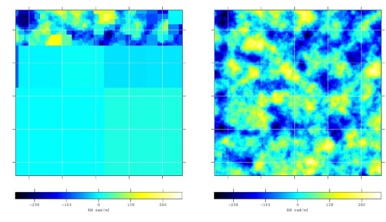
Figure 1: Right panel, a small part ($37\times 37$ kpc) of a typical realisation of a $RM$ map which is produced by a Kolmogorov-like magnetic field power spectrum for $k\geq k_{c}=0.8$ kpc^-1 and a magnetic field strength of 5 $\mu$G. Left panel, the $RM$ data used for the data matrix $\Delta_{i}$ is shown where we averaged arbitrary neighbouring points in order to reduce the number of independent points in a similar way as done later with the observational data.

In order to test our algorithm, we applied our maximum likelihood estimator to generated $RM$ maps with a known magnetic power spectrum $\varepsilon_{B}(k)$. Enßlin & Vogt (2003) give a prescription (their Eq. (37)) for the relation between the amplitude of $RM$, $|\hat{RM}(k_{\perp})|^{2}$, and the magnetic power spectrum in Fourier space

$$\varepsilon_{B}^{{\rm obs}}(k)=\frac{k^{2}}{a_{1}\,A_{\Omega}(2\pi)^{4}}\int_{0}^{2\pi}{\rm d}\phi\,\,|\hat{RM}(\@vec{k}_{\perp})|^{2}$$ (28)

or

$$|\hat{RM}(k_{\perp})|^{2}=\frac{a_{1}\,A_{\Omega}(2\pi)^{3}}{k^{2}}\varepsilon_{B}^{{\rm obs}}(k),$$ (29)

where $A_{\Omega}$ is the area $\Omega$ for which $RM$’s are actually measured and $a_{1}=a_{0}^{2}\,n_{{\rm e0}}^{2}\,L$, where $L$ is the characteristic depth of the Faraday screen.

As the Faraday screen, we assumed a box with sides being 150 kpc long and a depth of $L=300$ kpc. For simplicity, we assumed a uniform electron density profile with a density of $n_{{\rm e0}}=0.001$ cm^-3. For the magnetic field power spectra, we used

$$\varepsilon_{B}^{{\rm obs}}(k)=\left\{\begin{array}[]{ll}\frac{\varepsilon_{B}}{k_{0}^{1-\alpha}\,k_{c}^{2+\alpha}}\,k^{2}&\forall k\leq k_{c}\\ \frac{\varepsilon_{B}}{k_{0}}\left(\frac{k}{k_{0}}\right)^{-5/3}&\forall k\geq k_{c}\end{array}\right..$$ (30)

where the spectral index which was set to mimic Kolmogorov turbulence with energy injection at $k=k_{c}$, and

$$\varepsilon_{B}=\frac{\langle B^{2}\rangle}{8\pi}=\int_{0}^{k_{{\rm max}}}\!\!\!{\rm d}k\,\varepsilon_{B}^{{\rm obs}}(k),$$ (31)

where $k_{{\rm max}}=\pi/\Delta r$ is determined by the pixel size ($\Delta r$) of the $RM$ map used. The latter equation combined with Eq. (30) gives the normalisation $k_{0}$ in such a way that the integration over the accessible power spectrum will result in a magnetic field strength of $B$ for which we used 5 $\mu$G. We used a $k_{c}=0.8$ kpc^-1.

In order to generate a $RM$ map with the magnetic power spectrum $\varepsilon_{B}(k)$ for the chosen Faraday screen, we filled the real and imaginary part of the Fourier space independently with Gaussian deviates. Then these values were multiplied by the appropriate values given by Eq. (29) corresponding to their place in $k$-space. As a last step, an inverse Fourier transformation was performed. A typical realisation of such a generated $RM$ map is shown in Fig. 1.

For the analysis of the resulting $RM$ map only a small part of the initial map was used in order to reproduce the influence of the limited emission region of a radio source. We applied the Fourier analysis as described in Enßlin & Vogt (2003) to this part. The resulting power spectrum is shown in Fig. 2 as a dashed line in comparison with the input power spectrum as a dotted line.

The maximum likelihood method is numerically limited by computational power since it involves matrix multiplication and inversion, where the latter is a $N^{3}$ process. Thus, not all points of the many which are defined in our maps can be used. However, it is desirable to use as much information as possible from the original map. Therefore we chose to randomly average neighbouring points with a scheme which let to a map with spatially inhomogeneously resolved cells. The resulting map is highly resolved on top and lowest on the bottom with some random deviations which make it similar to the error weighting of the observed data. We used $N$ = 1500 independent points for the analysis. In the left panel of Fig. 1, the averaged $RM$ map which was used for the test is shown.

As a first guess for the maximum likelihood estimation, we used the power spectra derived by the Fourier analysis. The resulting power spectrum is shown as filled circles with 1-$\sigma$ error bars in Fig. 2. The input power spectrum and the power spectrum derived by the maximum likelihood estimator agree well within the one $\sigma$ level. Integration over this power spectrum results in a field strength of $(4.7\pm 0.3)\mu$G in agreement with the input magnetic field strength of $5\mu$G.

Figure 2: Power spectra for a simulated $RM$ map as shown in Fig. 1. The input power spectrum is shown in comparison to the one found by the Fourier analysis as described in Enßlin & Vogt (2003) and the one which was derived by our maximum likelihood estimator. One can see the good agreement within one $\sigma$ between input power spectrum and the power spectrum derived by the maximum likelihood method.

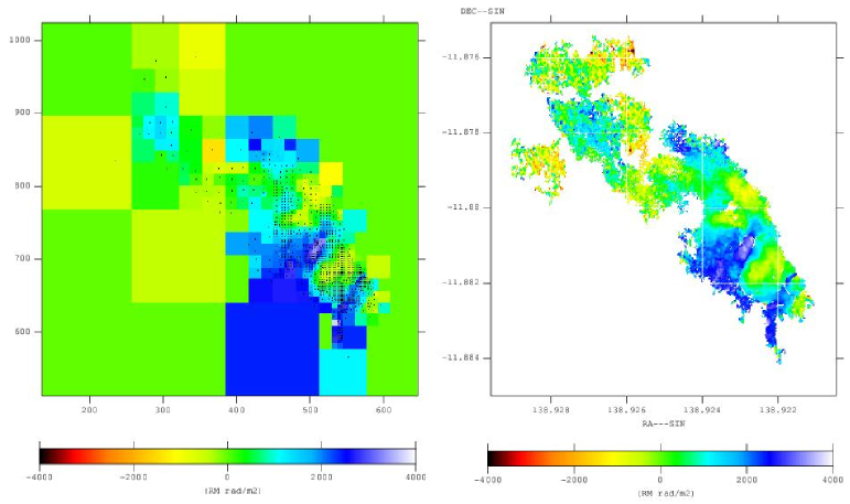
Figure 3: The final $RM$ map from the north lobe of Hydra A which was analysed with the maximum likelihood estimator; left: error weighted map. The dots indicate the coordinates which correspond to the appropriate error weighted $RM$ value, which resulted from averaging over the indicated area; right: original Pacman map. Note that the small scale noise for the diffuse part of the lobe is averaged out and only the large scale information carried by this region is maintained.

4 Application to Hydra A

4.1 The data $\@vec{\Delta}$

We applied this maximum likelihood estimator introduced and tested in the last sections to the Faraday rotation map of the north lobe of the radio source Hydra A (Taylor & Perley 1993). The data were kindly provided by Greg Taylor.

For this purpose, we used a high fidelity $RM$ map presented in Vogt et al. (2004) which was generated by the newly developed algorithm Pacman (Dolag et al. 2004) using the original polarisation data. Pacman also provides error maps $\sigma_{i}$ by error propagation of the instrumental uncertainties of polarisation angles. The Pacman map which was used is shown in the right panel of Fig. 3.

For the same reasons as mentioned in Sect. 3, we averaged the data. An appropriate averaging procedure using error weighting was applied such that

$$\overline{RM}_{i}=\frac{\sum_{j}{RM_{j}}/{\sigma^{2}_{j}}}{\sum_{j}{1}/{\sigma_{j}^{2}}},$$ (32)

and the error calculates as

$$\sigma^{2}_{\overline{RM}_{i}}=\frac{\sum_{j}\left({1}/{\sigma^{2}_{j}}\right)}{\left(\sum_{j}{1}/{\sigma_{j}^{2}}\right)^{2}}=\frac{1}{\sum_{j}{1}/{\sigma_{j}^{2}}}.$$ (33)

Here, the sum goes over the set of old pixels $\{j\}$ which form the new pixels $\{i\}$. The corresponding pixel coordinates $\{i\}$ were also determined by applying an error weighting scheme

$$\overline{x}_{i}=\frac{\sum_{j}{x_{j}}/{\sigma^{2}_{j}}}{\sum_{j}1/\sigma^{2}_{j}}\;\;\mbox{and}\;\;\overline{y}_{i}=\frac{\sum_{j}{y_{j}}/{\sigma^{2}_{j}}}{\sum_{j}1/\sigma^{2}_{j}}.$$ (34)

The analysed $RM$ map was determined by a gridding procedure. The original $RM$ map was divided into four equally sized cells. In each of these the original data were averaged as described above. Then the cell with the smallest error was chosen and again divided into four equally sized cells and the original data contained in the so-determined cell were averaged. The last step was repeated until the number of cells reached a defined value $N$. We decided to use $N=1500$. This is partly due to the limitation of computational power but also partly because of the desired suppression of small-scale noise by a strong averaging of the noisy regions.

The final $RM$ map which was analysed is shown in Fig. 3. The most noisy regions in Hydra A are located in the coarsely resolved northernmost part of the lobe. We chose not to resolve this region any further but to keep the large-scale information which is carried by this region.

4.2 The window function

As mentioned in Sect. 2.1, the window function describes the sampling volume and, thus, we have to find a suitable description for it based on Eq. 6. Hydra A (or 3C218) is located at a redshift of 0.0538 (de Vaucouleurs et al. 1991). For the derivation of the electron density profile parameter, we relied on the work by Mohr et al. (1999) done for ROSAT PSPC data while using the deprojection of X-ray surface brightness profiles as described in the Appendix A of Pfrommer & Enßlin (2004). Since Hydra A is known to exhibit a strong cooling flow as observed in the X-ray studies, we assumed a double $\beta$-profile and used for the inner profile $n_{{\rm e1}}(0)=0.056$ cm^-3 and $r_{c1}=0.53$ arcmin; for the outer profile we used $n_{{\rm e2}}(0)=0.0063$ cm^-3 and $r_{c2}=2.7$ arcmin and we applied a $\beta=0.77$.

Figure 4: The comparison of the integrated squared window function $f^{2}(r)$ (lines) with the $RM$ dispersion function $\langle RM^{2}(r)\rangle$ (open circles) and $\langle RM^{2}\rangle-\langle RM(r)\rangle^{2}$ (filled circles). Different models for the window function were assumed. In (a) $\alpha_{B}=1.0$, in (b) $\alpha_{B}=0.5$ and in (c) $\alpha_{B}=0.1$ were used, where the inclination angle $\theta$ of the source was varied. It can be seen that models for the window function with $\alpha_{B}=0.1\ldots 0.5$ and $\theta=10\degr\ldots 50\degr$ match the shape of the dispersion function very well.

Assuming this electron density profile to be accurately determined, there are two other parameters which enter in the window function. The first one is related to the source geometry. For Hydra A, a clear depolarisation asymmetry between the two lobes is observed, known as the Laing-Garrington effect (Garrington et al. 1988; Laing 1988) suggesting that the source is tilted from the $xy$-plane (Taylor & Perley 1993). In fact, the north lobe points towards the observer. In order to take this into account, we introduced an angle $\theta$ which describes the angle between the source and the $xy$-plane such that the north lobe points towards the observer. Taylor & Perley (1993) determine an inclination angle of $\theta=45\degr$.

The other parameter is related to the global magnetic field distribution which is assumed to scale with the electron density profile $B(r)\propto n_{{\rm e}}(r)^{\alpha_{B}}$. In a scenario in which an originally statistically homogeneously magnetic energy density gets adiabatically compressed, one expects $\alpha_{B}=2/3$. If the ratio of magnetic and thermal pressure is constant throughout the cluster then $\alpha_{B}=0.5$. However, $\alpha_{B}$ might have any other value. Dolag et al. (2001) determined an $\alpha_{B}=0.9$ for the outer regions of the cluster Abell 119.

In order to constrain the applicable ranges of these quantities, one can compare the integrated squared window function with the $RM$ dispersion function $\langle RM(r_{\perp})^{2}\rangle$ of the $RM$ map used since

$$\langle RM^{2}(r_{\perp})\rangle\propto\int_{-\infty}^{\infty}{\rm d}z\,f^{2}(r_{\perp},z),$$ (35)

as stated by Eq. (24) of Enßlin & Vogt (2003). Therefore, we compared the shape of the two functions. The result is shown in Fig. 4. For the window function, we used three different $\alpha_{B}=0.1,0.5,1.0$ and for each of these, five different inclination angles $\theta=0\degr,10\degr,30\degr,45\degr$ and $60\degr$ were employed, although the $\theta=0\degr$ is not very likely considering the observational evidence of the Laing-Garrington effect as observed in Hydra A by Taylor & Perley (1993). The different results are plotted as lines of different style in Fig. 4. The filled and open dots represent the $RM$ dispersion function. The solid circles indicate the binned $\langle RM^{2}\rangle$ function. The open circles represent the binned $\langle RM^{2}\rangle-\langle RM\rangle^{2}$ function, which is cleaned of any foreground $RM$ signals.

From Fig. 4, it can be seen that models with $\alpha_{B}=1.0$ or $\theta>50\degr$ are not able to recover the shape of the $RM$ dispersion function and, thus, we expect $\alpha_{B}<1.0$ and $\theta<50\degr$ to be more likely.

5 Results and discussion

Based on the described treatment of the data and the description of the window function, first we calculated power spectra for various scaling exponents $\alpha_{B}$ while keeping the inclination angle at $\theta=45\degr$. For this investigation, we used as the number of bins $n_{l}=5$ which proved to be sufficient. For these calculations, we used $\epsilon<0.1$. The resulting power spectra are plotted in Fig. 5.

Figure 5: Power spectra for $N=1500$ and $n_{l}=5$. Different exponents $\alpha_{B}$ in the relation $B(r)\sim n_{e}(r)^{\alpha_{B}}$ of the window function were used. The inclination angle of the source was chosen to be $\theta=45\degr$.

In Fig. 5, one can see that the power spectrum derived for $\alpha_{B}=1.0$ has a completely different shape whereas the other power spectra show only slight deviation from each other and are vertically displaced, implying different normalisation factors, i.e. central magnetic field strengths which increase with increasing $\alpha_{B}$. The straight dashed line which is also plotted in Fig. 5 indicates a Kolmogorov-like power spectrum being equal to $5/3$ in our prescription. The power spectra follow this slope over at least one order of magnitude.

In Sect. 4.2, we were not able to distinguish between the various scenarios for $\alpha_{B}$ although we found that an $\alpha_{B}=1$ does not properly reproduce the measured $RM$ dispersion. However, the likelihood function offers the possibility to calculate the actual probability of a set of parameters given the data (see Eq. (1)). Thus, we calculated the log likelihood $\ln{\mathcal{L}}_{\@vec{\Delta}}(\@vec{a})$ value for various power spectra derived for the different window functions varying in the scaling exponent $\alpha_{B}$ and assuming the inclination angle of the source to be for all geometries $\theta=45\degr$. In Fig. 6, the log likelihood is shown as a function of the scaling parameter $\alpha_{B}$ used.

Figure 6: The log likelihood $\ln\mathcal{L}_{\@vec{\Delta}}(\@vec{a})$ of various power spectra assuming different $\alpha_{B}$ while using a constant inclination angle $\theta=45\degr$. $\alpha_{B}=0.1\ldots 0.8$ are in the plateau of maximum likelihood. The sudden decrease for $\alpha_{B}<0.1$ in the likelihood might be due to non-Gaussian effects becoming too strong.

As can be seen from Fig. 6, there is a plateau of most likely scaling exponents $\alpha_{B}$ ranging from 0.1 to 0.8. An $\alpha_{B}=1$ seems to be very unlikely for our model as already deduced in Sect. 4.2. The sudden decrease for $\alpha_{B}<0.1$ might be due to non-Gaussian effects. The magnetic field strength derived for this plateau region ranges from 9 $\mu$G to 5 $\mu$G. The correlation length of the magnetic field $\lambda_{B}$ was determined to range between $2.5$ kpc and $3.0$ kpc whereas the $RM$ correlation length was determined to be in the range of $4.5\ldots 5.0$ kpc. These ranges have to be considered as a systematic uncertainty since we are not yet able to distinguish between these scenarios observationally. Another systematic effect might be given by uncertainties in the electron density itself. Varying the electron density normalisation parameters ($n_{{\rm e1}}(0)$ and $n_{{\rm e2}}(0)$) leads to a vertical displacement of the power spectrum while keeping the same shape.

In order to study the influence of the inclination angle on the power spectrum, we used an $\alpha_{B}=0.5$, being in the middle of the most likely region derived. For this calculation, we used smaller bins and thus increased the number of bins to $n_{l}=8$. We calculated the power spectrum for two different inclination angles $\theta=30\degr$ and $\theta=45\degr$. The results are shown in Fig. 7 in comparison with a Kolmogorov-like power spectrum.

Figure 7: Power spectra for two different inclination angles $\theta=30\degr$ and $\theta=45\degr$ and an $\alpha_{B}=0.5$. For comparison a Kolmogorov-like power spectrum is plotted as a straight dashed line. One can see that the calculated power spectra follow such a power spectrum over at least one order of magnitude. Note that the error bars are larger than in Fig. 5 because smaller bin sizes were used.

As can be seen from Fig. 7, the power spectra derived agree well with a Kolmogorov-like power spectrum over at least one order of magnitude. For the inclination angle of $\theta=30\degr$, we derived the following field and map properties $B=5.7\pm 0.1\,\mu$G, $\lambda_{B}=3.1\pm 0.3$ kpc and $\lambda_{RM}=6.7\pm 0.7$ kpc. For $\theta=45\degr$, we calculated $B=7.3\pm 0.2\,\mu$G, $\lambda_{B}=2.8\pm 0.2$ kpc and $\lambda_{RM}=5.2\pm 0.5$ kpc. The value of the log likelihood $\ln\mathcal{L}$ was determined to be slightly higher for the inclination angle of $\theta=30\degr$. The flattening of the power spectra for large $k$s can be explained by small-scale noise which we did not model separately.

Although the central magnetic field strength decreases with decreasing scaling parameter $\alpha_{B}$, the volume-integrated magnetic field energy $E_{B}$ within the cluster core radius $r_{{\rm c2}}$ increases. The volume-integrated magnetic field energy $E_{B}$ is calculated as follows

$$E_{B}=4\pi\int_{0}^{r_{{\rm c2}}}{\rm d}r\,r^{2}\,\frac{B^{2}(r)}{8\pi}=\frac{B_{0}^{2}}{2}\int_{0}^{r_{{\rm c2}}}{\rm d}r\,r^{2}\,\left(\frac{n_{{\rm e}}(r)}{n_{{\rm e0}}}\right)^{2\alpha_{B}},$$ (36)

where we integrate from the cluster centre to the core radius $r_{{\rm c2}}$ of the second, non-cooling flow, component of the electron density distribution.

We integrated the magnetic field profile for the various scaling parameters and the corresponding field strengths which we determined by our maximum likelihood estimator. The result is plotted in Fig. 8. The higher magnetic energies for the smaller scaling parameters which correspond to a lower central magnetic field strength are due to the higher field strength in the outer parts of the cool cluster core. This effect would be much more drastic if we had extrapolated the scaling $B(r)\propto n_{\rm e}(r)^{\alpha_{B}}$ to larger cluster radii and integrated over a larger volume.

Figure 8: The integrated magnetic field energy $E_{B}$ within the cluster core radius $r_{\rm c2}$ for the various scaling parameters $\alpha_{B}$ also used in Fig. 6 and the corresponding central magnetic field strength $B_{0}$ as determined by our maximum likelihood estimator.

6 Conclusions

We presented a maximum likelihood estimator for the determination of cluster magnetic field power spectra from $RM$ maps of extended polarised radio sources. We introduced the covariance matrix for $RM$ under the assumption of statistically homogeneously-distributed magnetic fields throughout the Faraday screen. We successfully tested our approach on simulated $RM$ maps with known power spectra.

We applied our approach to the $RM$ map of the north lobe of Hydra A. We calculated different power spectra for various window functions being especially influenced by the scaling parameter between electron density profile and global magnetic field distribution and the inclination angle of the emission region. The scaling parameter $\alpha_{B}$ was determined to be most likely in the range of $0.1\ldots 0.8$.

We realised that there is a systematic uncertainty in the values calculated due to the uncertainty in the window parameter itself. Taking this into account, we deduced for the central magnetic field strength in the Hydra A cluster $B=(7\pm 2)\,\mu$G and for the magnetic field correlation length $\lambda_{B}=(3.0\pm 0.5)$ kpc. If the geometry uncertainties could be removed, the remaining statistical errors are an order of magnitude smaller. The difference of these values to the ones found in an earlier analysis of the same dataset of Hydra A which yielded $B=12\mu$G and $\lambda_{B}=1$ kpc (Vogt & Enßlin 2003) is a result of the improved $RM$ map using the Pacman algorithm (Dolag et al. 2004; Vogt et al. 2004) and a better knowledge of the magnetic cluster profile, i.e. here $\alpha_{B}\approx 0.5$ (instead of $\alpha_{B}=1.0$ in Vogt & Enßlin 2003). However, the magnetic field strength found in Hydra A supports the trend of relatively large magnetic fields derived for cooling flow clusters from RM measurements reported in the literature.

The cluster magnetic field power spectrum of Hydra A follows a Kolmogorov-like power spectrum over at least one order of magnitude. However, from our analysis it seems that there is a dominant scale $\sim$ 3 kpc at which the magnetic power is concentrated.