• When Darwin Met Einstein: Gravitational Lens Inversion with Genetic Algorithms

  Brendon J. Brewer & Geraint F. Lewis
  Institute of Astronomy, School of Physics, University of Sydney, NSW 2006, Australia
  Email: brewer,gfl@physics.usyd.edu.au

  Abstract: Gravitational lensing can magnify a distant source, revealing structural detail which is normally unresolvable. Recovering this detail through an inversion of the influence of gravitational lensing, however, requires optimisation of not only lens parameters, but also of the surface brightness distribution of the source. This paper outlines a new approach to this inversion, utilising genetic algorithms to reconstruct the source profile. In this initial study, the effects of image degradation due to instrumental and atmospheric effects are neglected and it is assumed that the lens model is accurately known, but the genetic algorithm approach can be incorporated into more general optimisation techniques, allowing the optimisation of both the parameters for a lensing model and the surface brightness of the source.

  Keywords: Gravitational lensing — methods: numerical

1 Introduction

Gravitational lensing is an important astrophysical tool, mapping the distribution of matter on many scales and revealing typically unresolved detail of distant sources through magnification [see Kochanek et al. (2004) for a review of lensing physics]. Early studies concentrated upon the properties of multiply imaged quasars to determine the underlying mass distribution within the lensing galaxy. However, the point-like nature of quasars (which results in point-like images) present only a limited amount of constraints on the lensing mass distribution, with a number of degenerate solutions able to explain the observed configuration (Kent & Falco 1988; Schneider et al. 1988; Kochanek 1991).

If the source in a gravitational lensing is extended, the resulting image is also extended and each resolution element effectively provides a constraint on any modelling. Any modelling, however, becomes more complex than the simple case of point-like lensing which asks the question “what distribution of mass in the lensing can account for the observed image locations and brightnesses?”. With an extended source, the question has to be rephrased as “what distribution of mass in the lensing galaxy and distribution of brightness in the source can account for the observed image configuration?”. To answer this question, more novel approaches to gravitational lensing modelling have been undertaken (Kochanek, Blandford, Lawrence, & Narayan 1989; Kochanek & Narayan 1992; Ellithorpe, Kochanek, & Hewitt 1996; Wallington, Kochanek, & Narayan 1996; Warren & Dye 2003; Wucknitz 2004; Wayth et al. 2005; Dye & Warren 2005). These techniques typically determine not only the mass distribution in the lensing galaxy, but also the surface brightness distribution in the source.

Given the form of the lens and the source, it is relatively straightforward to compute the resultant image by using a simple ray tracing method. The inverse problem, which is what occurs in practice, is much more difficult to solve. Furthermore, inverse problems are fraught with the question of solution uniqueness. To this end, it is advisable to tackle a particular problem with a range of inversion techniques and compare the various outcomes; if all approaches converge to the same result, some faith can be given to the overall solution. Currently, the repertoire of gravitational lens inversion techniques is relatively small and so this paper presents an alternative approach to gravitational lens modelling, utilising genetic algorithms to reconstruct the source. This initial investigation of this approach, the effects of image degradation through instrumental and atmospheric effects (i.e. seeing) are neglected, although these can be implemented in a straightforward fashion. The approach is described in detail in Section 2, considering a perfect, noiseless image. Section  3 discusses the influence of the various parameters influencing the inversion technique, also considering reconstruction of noisy images. Section 4 considers the more general problem of the optimization of both the source surface brightness distribution and the parameters governing the mass distribution in the lensing galaxy. This paper closes with the conclusions which are presented in Section 5.

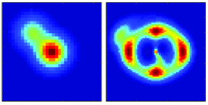
Figure 1: The left-hand panel presents the artificial source utilised in this study, while the right-hand panel presents the image of this source as seen through the model gravitational lens (see section 2.2.2). Note that these images as on different scales, with the source panel being half the width of the image panel. The source is defined on a grid of 32$\times$32 pixels, whereas the resultant image is 64$\times$64 pixels. For observed gravitational lens images, the image would be $\sim 3$ arcseconds on a side, corresponding to a pixel scale of $0.05$ arcseconds per pixel. The corresponding source plane region possesses an image scale of 0.025 arcseconds per pixel and a side length of 0.8 arcseconds.

2 Approach

2.1 Genetic Algorithms

Genetic algorithms are an approach to problems of optimisation that take their inspiration from evolutionary biology [for a popular review of genetic algorithms and other aspects of biological computing, see Levy (1993)]. The basic approach, presented in some detail in Charbonneau (1995), mimics the evolutionary struggle of life, with different individuals having different probabilities of passing on their genes to the next generation, with the probabilities dependent on the environment and the physical characteristics of the organism (which in turn depend on the genes). Humans have long used a basic knowledge of heredity to breed for desirable traits in animals and crops, even before Charles Darwin proposed his theory of natural selection (Darwin 1859). Genetic algorithms take this idea and apply it by “breeding” better solutions to the problem at hand.

In terms of the algorithmic approach, several features are required;

• Encoding: Each potential solution to a problem is encoded into a genome. This is often represented as a series of digits, but can be a simple bit string.

• Expression: This decodes the information in the genome into a phenotype. For many applications, this decodes the genome into a series of real numbers that are used as parameters for a particular model.

• Fitness evaluation: This compares the phenotype of the genome to the problem, assigning a quantitative measure of the goodness of fit of the potential solution (e.g. a standard $\chi^{2}$ measurement).

With these, an initial population of genomes, each representing a potential solution to the problem at hand, can be generated. Typically this involves assigning each genome with a random sequence of digits or bits. In evolving this population to the next generation, several steps are involved:

a) Ranking & Selection Pressure: The goal of a genetic algorithm is to produce subsequent generations of solutions with greater fitness by ensuring that the fittest member of a current population to pass their genetic material onto to the next generation. As noted by Charbonneau (1995), as evolution proceeds, the average and maximum fitness of a population continually increases. The spread in fitness, however, decreases, with the overall population becoming homogeneous. With such uniform fitness in a population, simple selection on fitness alone effectively samples randomly from the population and evolution stalls. To circumvent this, selection must be made relative to the current population. To this end, the population is ranked in terms of its fitness, with the least fit being assigned a value of 0, whereas the most fit possesses a value of 1. Members are selected from this current generation with a probability dependent upon their ranking, such that

$$p\propto(ranking)^{\beta}$$ (1)

where $\beta$ is called the selection pressure. If $\beta=0$, the probability for selection is uniform throughout the population, while larger values of $\beta$ preferentially select only the fittest members in the population.

b) Elitism: The fittest member of the current generation is cloned and represents the first member of the next generation. This ensures that the maximum fitness of subsequent generations can never fall.

c) Breeding: Further members of the next generation are produced by breeding the members of the current generation, with the genetic information of the current population used to determine the genomes of the next. The probability that an individual will breed is based upon its ranking and the selection pressure as outlined previously. Two breeding strategies are adopted, asexual and sexual reproduction. With asexual reproduction, a selected member of the current generation is cloned, preserving the genetic information, to provide a new member of the next generation. In sexual reproduction, two members of the current generation are selected and a new individual is formed with the combination of their genetic material; a random portion of the genome of one parent is “copied and pasted” over the corresponding part of the other parent’s genome to produce the resulting offspring genome; this allows the genetic material of successful organisms to mix. Whether the creation of an offspring is due to sexual reproduction is determined randomly, with a pre-defined probability referred to as the crossover rate.

d) Mutation: A population which reproduces purely asexually rapidly becomes dominated by a single genome and evolution grinds to a halt. Random mutations in the genetic sequence can drive evolution beyond this point, increasing diversity in a population  The probability that a particular digit in the genetic sequence is mutated (straight after breeding) is determined by the mutation rate.

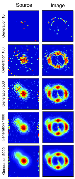
Figure 2: An example of the evolutionary sequence obtained with the genetic algorithm reconstruction of an idealised gravitational lens system. The left-hand panel displays the source plane surface brightness distribution at 10, 100, 500, 1000 and 5000 generations, while the right-hand panel presents the resulting image plane distribution. It is clear, when comparing to Figure 1, that the fitness of the solution is increasing with each generation. Note that the vertical noise at the edge of the source plane correspond to regions which are not mapped into the image plane and so do not contribute to the overall fitness of the image reconstruction.

The breeding and mutation are continued until a new generation is formed, and the entire initial generation is culled. Steps a) through d) are then repeated, with subsequent generations exhibiting fitter solutions to the problem. The evolution is terminated when an appropriate fitness criterion is satisfied.

Charbonneau (1995) and Hakala (1995) presented some of the earliest applications of genetic algorithms in astronomy, with the former detailing a freeware algorithm (PIKAIA) . These early studies focused upon the fitting of light curves and galactic rotation curves (Charbonneau 1995), and constraining accretion stream mapping in eclipsing polars (Hakala 1995), but since then the application of genetic algorithms has been used in the design of filters and filter systems (Offer & Bland-Hawthorn 1998; Bailer-Jones 2004), modelling the structure of the galaxy (Larsen & Humphreys 2003), the signature of gamma ray bursts (Portegies Zwart & Totani 2001), solar oscillations (Fletcher, Chaplin, & Elsworth 2003) and even the scheduling of telescopes (Gómez de Castro & Yáñez 2003).

2.2 Gravitational Lens Inversion

2.2.1 Encoding & Phenotyping

For the purposes of this project, each individual genome was taken to be a string of 1024 characters. The expressed genome (the phenotype) represented 32$\times$32 pixels, where each pixel could take a value between 0 and $F_{max}$. This pixel array represents the surface brightness distribution of the source. Such an encoding ensures the surface brightness is subject to a positivity constraint [this is not the case of some other inversion approaches e.g. Warren & Dye (2003)]. In the coming simulations, $F_{max}=255$.

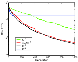
Figure 3: The influence of the mutation rate on fitness as a function of generation. The box in this panel (and in subsequent figures) denotes the different values of parameter adopted. Note, this figure presents $fitness^{-1}$ as defined in Equation 4. A reasonable rate of mutation is needed to stimulate progress in the population by providing random variations for selection to act upon. However, if the mutation rate is too high, any “good” genomes will be severely affected by too many mutations. The black curve is for the adopted mutation rate of $10^{-3}$.

2.2.2 Gravitational Lens Model

The scaled lensing equations relating a position $(x,y)$ in the image plane to the corresponding point $(x_{s},y_{s})$ in the source plane [see Wambsganss (1998)] can be written in terms of a potential $\phi(x,y)$ (related to the mass distribution of the lens) such that

$$\begin{array}[]{rcl}x_{s}=x-\frac{\partial\phi}{\partial x}|_{(x,y)}\\ \\ y_{s}=y-\frac{\partial\phi}{\partial y}|_{(x,y)}\end{array}$$ (2)

The gravitational lens potential was chosen to be the three parameter pseudo-isothermal elliptic potential (Kochanek, Blandford, Lawrence, & Narayan 1989) of the form

$$\phi(x,y)=b\sqrt{r_{c}^{2}+(1-\epsilon)x^{2}+(1+\epsilon)y^{2}}$$ (3)

where $r_{c}$ is the core radius of the potential, $\epsilon$ is the ellipticity and $b$ is an overall normalisation factor (typically linked to the velocity dispersion of the lensing galaxy). While the determination of these parameters is the typical goal of many analyses of gravitational lenses, in this intial examination of genetic algorithms, it is assumed that the model is fixed and its parameters are known. In other words, the goal is to find the source profile, given the observed image and the form of the lens. The adopted values for the lens parameters were $b=0.5$, $\epsilon=0.25$ and $r_{c}=0.1$. The full optimisation problem of the source profile and model parameters will be discussed in Section 4.

2.2.3 Fitness Determination

To test the effectiveness of the genetic algorithmic approach to gravitational lens inversion, an example solution was defined. This consisted of two offset Gaussian profiles of differing heights and is displayed graphically in the left-hand panel of Figure 1, while the image of this source as seen through the lensing potential outlined previously appears in the right-hand panel. The image of the source is realised upon a 64$\times$64 grid.

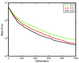
Figure 4: As for Figure 3, but detailing the influence of cross-over rate on fitness as a function of generation.

In determining the fitness of a particular genome, its expressed phenotype is used to represent a potential source. This is mapped, via the lens model, to produce the resulting image configuration. This is then compared to the ideal image (Figure 1) and the assigned fitness was chosen to be the reciprocal of the sum of the squared differences between the reconstructed image and the observed image:

$$fitness=\frac{1}{\sum_{i=1}^{64}\sum_{j=1}^{64}(m_{ij}-p_{ij})^{2}}$$ (4)

where $m_{ij}$ are the pixel brightnesses of the model generated from the genome and $p_{ij}$ are the pixel brightnesses of the “observed” image. Clearly, in the absence of noise, the sum of the squared differences for a perfect genome is zero and hence the fitness is infinite. Of course, for a real gravitational lens system, this ideal image will be replaced with a noisy observed image. Simulations of the genetic algorithm considering the influence of noise, will be discussed in Section 3.2.

3 Results

Examples of the source reconstructions achieved with the genetic algorithm are presented in Figure 2. These were produced by optimising the source profile, assuming that the correct lens model was known. From top to bottom, each pair of panels presents a snapshot of the evolution, showing the fittess member of a generation. The left-hand panel graphically presents the surface brightness of the source (the genome), whereas the right-hand panel presents the resultant image configuration (the phenotype). Clearly, as the population is evolved to older generations, the accuracy of the solution increases (compare the source and image configuration at Generation 5000 to Figure 1). Note that the ‘noisy’ pixels along the vertical sides of the source reconstruction in Figure 2 correspond to regions which are not mapped into the image region and so does not contribute to the overall fitness of the solution.

3.1 Evolutionary Parameters

There are several parameters that can affect the performance of a genetic algorithm. It is important to find a set of parameters which is good at finding a solution quickly, since it can be a computationally expensive task to run for many generations. Also it may be necessary to evolve the population many times, in which case it is very important to minimise the time required to find a satisfactory solution. There are several factors which have the potential to influence this performance, and the four which are investigated here are the mutation rate, the crossover rate, the size of the population and the selection pressure, which is the relationship between the fitness score and the probability of being selected for breeding.

It is known that there are interactions between these parameters such that, for example, the answer to the question “what mutation rate should I use?” depends on the values of the other parameters (Charbonneau 1995). It is also highly dependent on the nature of the problem at hand. Therefore, the best that can be hoped for is some general picture of what order of magnitude these parameters should be.

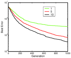
Figure 5: As for Figure 3, but detailing the influence of selection pressure on the fitness as a function of generation.

To test the dependency of the genetic alorithmic approach on the adopted parameters, an initial reconstruction was undertaken with the following parameters; the crossover rate was set to 0.9, the population size was 50, the mutation rate was set to $10^{-3}$ and the selection pressure was set to 10 (these were ‘good’ values found after much painstaking trial and error). In the following sections, one of these parameters was varied, while the others were kept fixed, allowing the influence of the varied parameter to be determined.

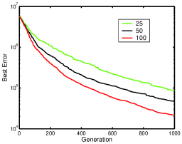
Figure 6: As for Figure 3, but detailing the influence of population size on the fitness as a function of generation.

3.1.1 Mutation

Figure 3 presents the evolution of the “Best Error” (defined as $fitness^{-1}$) of the fittest member of a population as a function of generation for several differing mutation rates. Clearly, if the mutation rate is low $(10^{-4})$ then the genome evolves slowly, but shows steady improvement. Increasing the rate of mutation increases the rate of improvement in the genome. However, this cannot continue indefinitely; as can be seen, a large mutation rate $(10^{-2})$ results in a rapid increase in improvement initially, after a short time the evolution stagnates. This is because for a mutation rate of 0.01 and a genome length of 1024, on average there are about 10 mutations per generation on each individual, and this is enough to outweigh any improvements that have evolved through selection. Hence, a little mutation is a good thing, but too much mutation is not. A general rule of thumb is that a good mutation rate is one which will give about 1 mutation over the whole genome.

3.1.2 Cross-over Rate

Figure 4 presents the results of varying the cross-over rate on the rate of improvement of the genome. For the three trial values of 0.1, 0.5 and 0.9, there is very little difference on the rate of improvement over time. Clearly, the algorithm is generally insensitive to the adopted value of the cross-over rate.

3.1.3 Selection Pressure

Figure 5 presents the influence of the selection pressure, $\beta$, on the rate of improvement of the fittest genome. Three $\beta$ values of 1, 5 and 10 were trialed; remember that $\beta=0$ ensures a uniform selection probability for breeding from a population (i.e. no selection pressure at all), whereas larger values preferentially selected the fittest members for breeding. For the adopted values, there was a definite advantage in using a $\beta$ value bigger than 1, but only a slight difference in performance between $\beta$ = 5 and $\beta$ = 10.

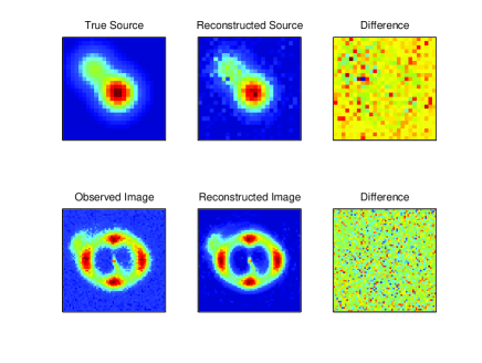
Figure 7: The results of the genetic algorith reconstruction using the noisy image after 5000 generations.

3.1.4 Population Size

The number of individuals in the population can also be varied, and the influence of changing population size is presented in Figure 6. Clearly larger populations have a larger spread in genetic variation and it is seen that the larger populations do evolve more rapidly. From a computational point of view, however, smaller populations result in a significant speed advantage, with less calculations required per generation.

In fact, as the time taken for each generation is roughly proportional to the population size, the larger genetic variability seen in larger population can be outweighing the time required to calculate the fitness of a population.

3.2 Source Reconstruction & Noise

In real life, astronomical images are always contaminated with some random noise, arising from sources such as thermal fluctuations in electronics, the effects of the atmosphere, and even photon counting noise if the source is faint (a feature that is shared by a number of extended gravitational lenses). Therefore it is worthwhile to test how the genetic algorithm performs when the observed image is contaminated with noise.

Including ‘errors’ into the observed image also sets a meaningful criterion to decide whether a particular reconstruction is “good enough”. This criterion will be met if the reconstructed image matches the observed image to within the statistical error level set by the noise. For this test, a normally distributed random variable with $\sigma$ = 5 was added to each pixel in the observed image, creating the noisy image shown in the lower left-hand panel of Figure 7.

When the genetic algorithm was run, the error vs. time plot (Figure 8) flattened out at a much higher value. This was not surprising, because in this case it is not possible to have a source that reproduces the observed image exactly, with its random fluctuations between neighbouring pixels. The additional panels in Figure 7 presents the reconstructed image and source profile, as well as the difference between these and the true source and corresponding image; these are consistent with the input noise characteristics.

This process can be thought of as a curve-fitting problem in 2 dimensions, with $64^{2}$ data points (the observed image), each with an error bar of 5 units. The aim is to fit this data using a model that has $32^{2}-N$ free parameters (each pixel of the source; note $N\sim 80$ corresponds to those pixels in the source grid which are not lensed into the final image, and hence are not true free parameters; see Figure 2). The chi-squared statistic for this fit (with degrees of freedom equal to the number of constraints minus the number of free paramaters in the model, i.e. $64^{2}-32^{2}+80$) is given by

$$\chi^{2}=\sum_{i=1}^{64}\sum_{j=1}^{64}\frac{(m_{ij}-p_{ij})^{2}}{\sigma^{2}}=\frac{1}{\sigma^{2}*fitness}$$ (5)

Hence, a reconstruction is statistically good (within 1$\sigma$) if the sum of the squared differences between the observed image and the image of the reconstructed source is within $\sigma^{2}\times(\nu\pm\sqrt{2\nu})$, where $\nu$ is the number of degrees of freedom. (Press et al. 1992) Hence, a good fit corresponds to a value in the range of $78800\pm 1985$. The genetic algorithm was able to reduce the error to $\sim 82000$, and so recovered an acceptable fit to the noisy image.

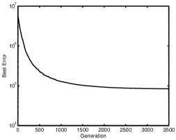
Figure 8: Error of the fittest solution vs generation for the noisy image. Notice that it does not tend to zero, as a perfect reconstruction of this image is impossible.

4 Full Optimisation

4.1 Lens Parameters in the Genome

In general, the goal of gravitational lens reconstruction is to determine both the surface brightness of the source and the parameters describing the mass distribution in the deflecting galaxy. How can the genetic algorithmic approach be generalised to tackle this problem? One idea that was tried was incorporating the lens parameters as part of the potential solutions to the problem, by encoding them in the genomes. Then, the evolution would hopefully select individuals whose lens parameters were close to the right values, and then proceed to optimise the source pixels. The result of this approach was not very successful. What actually occurred was that early on, a particular value of parameters was “locked on” and became dominant in the population. Then, the sources were optimised for those (incorrect) values, and there was little hope in ever getting to the right values. This was because any change to the parameter values would require a huge chance jump in the sources in order to gain a higher fitness than what had already evolved.

4.2 Direct Search Method

While incorporating the lens parameters in the genome was found not to be successful, an approach using a started direct search, independent of the genetic algorithm, was found to be successful. For the purposes of this study, simple one-dimensional searches were employed, although the technique can be easily generalised into higher dimensional searches.

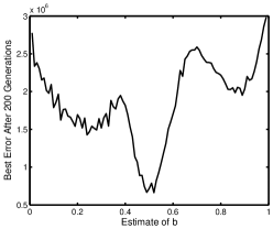
Figure 9: The best error after 3500 generations as a function of the value of $b$. Clearly, a good reconstruction of the image is only possible if the value of $b$ is close to the true value of 0.5.

An example of such a one-dimensional search is presented in Figure 9, in which $r_{c}$ and $\epsilon$ were held at their optimum value, and a suite of reconstructions were undertaken with differing values of $b$. This figure presents the residual of the fittest solution of the population after 3500 generations. This clearly reveals that a good reconstruction is only possible if $b$ is very close to the correct value of 0.5.

The major disadvantage of this approach is its computational inefficiency. Each point in Figure 9 required the genetic algorithm to be run over 3500 generations, which takes about 10 minutes on a modern desktop computer. However, it was noticed that even after a small number of generations, the correct value of $b$ was “winning the race” and so a smaller number of generations can be run to determine the interesting regions of parameters space for for further exploration. To illustrate this, Figure 10 presents the same result as Figure 9, using only 200 generations rather than 3500. This obviously has a significant computational advantage.

Calculating each point in Figures 9 and 10 required one run of the genetic algorithm, and the population was reset each time such that the initial genomes are sequences of zeros (corresponding to black pixels). However, if each point in these figures are calculated sequentially, the populations need not be reset as the solution to the previous point already contains fairly good solution, but for a slightly different $b$-value. Then the GA is given a “head start” in trying to improve the solution, effectively tweaking the previous solution to produce a new solution. This results in a dramatic smoothing out of the figures (Figure 11), and allows the parameter to be calculated correctly to and accuracy about 3 significant figures in only 200 generations.

As noted earlier, it should be possible to simply generalise this one-dimensional method to include more than one free parameter, either by using a large grid search (which may take a long time, although it is straightforward to devise a parallel computing scheme to do this, since each run can be done independently of the others), or by using a multidimensional minimisation method such as Powell’s method.

5 Conclusions

This paper has introduced a new technique for the inversion of gravitational lensed images of extended sources. This utilises genetic algorithms to evolve an optimal source for a particular gravitational lens model. It is seen that this approach successfully recovers the source configuration of an idealised gravitational lens system. Furthermore, it was demonstrated that this genetic algorithmic approach successfully recovers the source profile in the presence of noise and can be incorporated into more general gravitational lens optimisation schemes. This initial investigation has considered only a simple model of gravitational lensing, neglecting detailed aspects of true gravitational lens systems, such as various sources of noise and image smearing due to instrumental and atmospheric effects. However, due to the forward mapping of this approach, these can be added in a straight forward fashion, providing an inversion technique that can be applied to observed gravitational lens systems. Due to the limited time-frame of this initial project, these aspects of the algorithm will be left as further work.

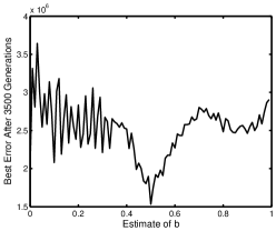
Figure 10: Best error after 200 generations as a function of the value of $b$. Note that the evolution is proceeding at a faster rate, even at this early stage, if the lens parameters are correct.

The most time consuming part of the genetic algorithmic approach is the calculation of the fitness of each member in a generation, scaling with the size of the population. For a particular genome, however, the calculation of the fitness is independent of the other members of the generation. This leads to a simple parallelisation of the approach, with the fitness calculation farmed out to individual processors. Furthermore, genetic evolution can be driven harder via the inclusion of parasitic organisms or ‘black sheep’ (Bobinger 2000), speeding up the evolution of the genome to fitter solutions and preventing evolutionary stagnation; these too will be incorporated into fuller version of this inversion technique.

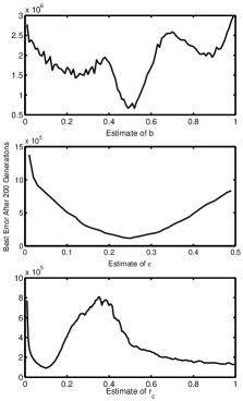
Figure 11: Best error after 200 generations as a function of the estimated values of the parameters (with the other two fixed at the correct values). The minima of the plots are all at the true values of the parameters. These figures were calculated without resetting the population after each 200 generations.

6 Acknowledgements

Aspects of this research were undertaken as a third year special project at the University of Sydney.

References

- Bailer-Jones (2004) Bailer-Jones, C. A. L. 2004, A&A, 419, 385
- Bobinger (2000) Bobinger, A. 2000, A&A, 357, 1170
- Charbonneau (1995) Charbonneau, P. 1995, ApJS, 101, 309
- Cohen & Stewart (2000) Cohen, J. & Stewart, I. 2000, The Collapse of Chaos, Penguin Books
- Darwin (1859) Darwin, C. 1859, Origin of Species, Penguin Books
- Dye & Warren (2005) Dye, S., Warren, S. J., Submitted to ApJ, astro-ph/0411452
- Ellithorpe, Kochanek, & Hewitt (1996) Ellithorpe J. D., Kochanek C. S., Hewitt J. N., 1996, ApJ, 464, 556
- Fletcher, Chaplin, & Elsworth (2003) Fletcher, S. T., Chaplin, W. J., & Elsworth, Y. 2003, MNRAS, 346, 825
- Gómez de Castro & Yáñez (2003) Gómez de Castro, A. I. & Yáñez, J. 2003, A&A, 403, 357
- Goździewski, Konacki, & Maciejewski (2003) Goździewski, K., Konacki, M., & Maciejewski, A. J. 2003, ApJ, 594, 1019
- Hakala (1995) Hakala, P. J. 1995, A&A, 296, 164
- Kent & Falco (1988) Kent, S. M. & Falco, E. E. 1988, AJ, 96, 1570
- Kochanek (1991) Kochanek, C. S. 1991, ApJ, 373, 354
- Kochanek, Blandford, Lawrence, & Narayan (1989) Kochanek, C. S., Blandford, R. D., Lawrence, C. R., & Narayan, R. 1989, MNRAS, 238, 43
- Kochanek & Narayan (1992) Kochanek C. S., Narayan R., 1992, ApJ, 401, 461
- Kochanek et al. (2004) Kochanek C. S., Schneider P., Wambsganss J., Part 2 of Gravitational Lensing: Strong, Weak & Micro, Proceedings of the 33rd Saas-Fee Advanced Course, G. Meylan, P. Jetzer & P. North, eds (Springer-Verlag: Berlin)
- Larsen & Humphreys (2003) Larsen, J. A. & Humphreys, R. M. 2003, AJ, 125, 1958
- Levy (1993) Levy, S. 1993, Artificial Life: A Report from the Frontier Where Computers Meet Biology, Vintage Books USA
- Metcalfe (1999) Metcalfe, T. S. 1999, AJ, 117, 2503
- Offer & Bland-Hawthorn (1998) Offer, A. R. & Bland-Hawthorn, J. 1998, MNRAS, 299, 176
- Portegies Zwart & Totani (2001) Portegies Zwart, S. F. & Totani, T. 2001, MNRAS, 328, 951
- Press et al. (1992) Press W. H., Teukolsky S. A., Vetterling W. T., Flannery B. P., 1992, Numerical Recipes, Cambridge
- Schneider et al. (1988) Schneider, D. P., Turner, E. L., Gunn, J. E., Hewitt, J. N., Schmidt, M., & Lawrence, C. R. 1988, AJ, 95, 1619
- Wallington, Kochanek, & Narayan (1996) Wallington, S., Kochanek, C. S., & Narayan, R. 1996, ApJ, 465, 64
- Wambsganss (1998) Wambsganss J., 1998, Living Reviews in Relativity, 1, 12
- Warren & Dye (2003) Warren, S. J. & Dye, S. 2003, ApJ, 590, 673
- Wayth et al. (2005) Wayth, R. B., Warren, S. J., Lewis, G. F. & Hewett, P. C., MNRAS Submitted, astro-ph/0410253
- Wucknitz (2004) Wucknitz O., 2004, MNRAS, 349, 1