Systematic errors in weak lensing: application to SDSS galaxy-galaxy weak lensing
Abstract
Weak lensing is emerging as a powerful observational tool to constrain cosmological models, but is at present limited by an incomplete understanding of many sources of systematic error. Many of these errors are multiplicative and depend on the population of background galaxies. We show how the commonly cited geometric test, which is rather insensitive to cosmology, can be used as a ratio test of systematics in the lensing signal at the 1 per cent level. We apply this test to the galaxy-galaxy lensing analysis of the Sloan Digital Sky Survey (SDSS), which at present is the sample with the highest weak lensing signal to noise and has the additional advantage of spectroscopic redshifts for lenses. This allows one to perform meaningful geometric tests of systematics for different subsamples of galaxies at different mean redshifts, such as brighter galaxies, fainter galaxies and high-redshift luminous red galaxies, both with and without photometric redshift estimates. We use overlapping objects between SDSS and the DEEP2 and 2SLAQ spectroscopic surveys to establish accurate calibration of photometric redshifts and to determine the redshift distributions for SDSS. We use these redshift results to compute the projected surface density contrast around 259 609 spectroscopic galaxies in the SDSS; by measuring with different source samples we establish consistency of the results at the 10 per cent level (). We also use the ratio test to constrain shear calibration biases and other systematics in the SDSS survey data to determine the overall galaxy-galaxy weak lensing signal calibration uncertainty. We find no evidence of any inconsistency among many subsamples of the data.
keywords:
gravitational lensing – galaxies: distances and redshifts – galaxies: halos.1 Introduction
Recent years have seen tremendous progress in the detection of galaxy-galaxy weak lensing (Brainerd et al. 1996; Hudson et al. 1998; Fischer et al. 2000; Smith et al. 2001; McKay et al. 2001; Guzik & Seljak 2002; Hoekstra et al. 2003; Sheldon et al. 2004; Hoekstra et al. 2004; Seljak et al. 2005), the tangential shear distortion around galaxies due to their dark matter halos. Recent measurements of galaxy-galaxy weak lensing (Sheldon et al. 2004; Hoekstra et al. 2004; Seljak et al. 2005) demonstrate 20–30 detections. In light of the increasing statistical precision with which this effect is measured, it is important to revisit common sources of systematic error, which are currently at the 10 per cent level and therefore already dwarf the statistical error.
While galaxy-galaxy weak lensing is potentially a very powerful tool for studying the dark matter halo profiles around stacked foreground galaxies, it suffers from a large number of potential calibration biases. Because it involves measuring the projected surface density contrast,
| (1) |
averaged over stacked lens and source galaxies (where is the transverse separation from the lens galaxy), calibration biases may be introduced via both the tangential shear and the redshifts used to compute .
Here we introduce some of the notation that is used in this paper to describe the weak-lensing signal. We compute the 2-dimensional projected surface density contrast of stacked foreground galaxies as a function of transverse separation from those galaxies, where this separation is measured in comoving coordinates, using (with subscript referring to the lens, to the source), and , the product of the observed angular lens-source separation on the sky and the angular diameter distance at the lens redshift. We can then measure the surface density contrast, which is related to the projected mass density and its average value inside radius , , as follows:
| (2) |
The inverse critical surface density in comoving coordinates is defined by
| (3) |
in terms of angular diameter distances, and has the following properties: for a given lens redshift, it is zero for , then increases rapidly above until it flattens out as ; the asymptotic value for increases with .
For a full discussion of the errors that can be introduced in the shear computation, see Hirata et al. (2004), hereinafter H04. As shown there, several types of error can be introduced when computing the shear, including biases due to point-spread function (PSF) correction, noise rectification bias, and selection biases. These biases are considered in detail for the linear PSF correction method used in that paper. In this paper, we use a different PSF correction scheme, “re-Gaussianization,” which was introduced and tested in Hirata & Seljak (2003), and include a discussion of the effects of that choice on systematic error in the shear.
Because systematic errors in the shear computation have been well-studied, and statistical errors can be decreased to a fairly low level when data from large surveys such as the SDSS are used, systematic errors in the redshift distribution (and consequently, in ) are of much greater importance than they were previously. For the purposes of this paper, we will assume that lens redshifts are known to high precision via spectroscopy, so our concern is the source redshift distribution; as shown in Kleinheinrich et al. (2004), if the lens redshifts are also unknown, g-g weak lensing is not nearly as powerful a tool. Several common methods of determining the source redshift distribution are inadequate for precision cosmology due to previously unquantified systematic uncertainties that they introduce via their effects on ; this paper includes a study of the biases that may be introduced using these methods, and a comparison against a well-determined reference distribution.
In addition to biases introduced due to the redshift distribution, we also discuss systematics that can be introduced while computing the signal. These include biases due to intrinsic alignments, selection effects, and several other effects. One new effect not noted before is a problem with the determination of the sky flux near bright objects by the SDSS Photo pipeline that leads to the problem in detection of sources within about of bright objects (§6.3.7). This problem affects any galaxy-galaxy or cluster-galaxy weak lensing analysis using SDSS data.
Many of the sources of systematic errors discussed above are common to both weak lensing auto-correlation analysis and galaxy-weak lensing correlations (galaxy-galaxy lensing). Weak lensing auto-correlation analysis at present is limited by the statistical precision (see summaries in Refregier 2003b and Hoekstra 2003) and it is difficult to test for the presence of systematics within each data set. However, the size of these data sets is rapidly increasing, and in the near future systematic errors are likely to dominate the statistical errors. Understanding of weak lensing systematics is essential if one is to exploit the full potential of upcoming and planned surveys such as the CFHT Legacy survey (http://www.cfht.hawaii.edu/Science/CFHLS, Mellier 2001), Pan-Starrs (http://pan-starrs.ifa.hawaii.edu/, Kaiser et al. 2002, Kaiser 2004), LSST (http://www.lsst.org/lsst_home.html, Tyson 2002), and SNAP (http://snap.lbl.gov/, Rhodes et al. 2004, Massey et al. 2004, Refregier et al. 2004), some of which may reach statistical precision at the 0.1 per cent level.
Many of our systematic tests are done using the following method. Several authors (Jain & Taylor 2003, Bernstein & Jain 2004) have proposed geometric tests of dark energy using the fact that is an invariant of the projected lens mass distribution, and therefore must be the same when measured with two different source samples at different redshifts. The use of this fact to test the dark energy density and equation of state requires control of systematics at the 0.1 per cent level. Since systematics in weak lensing are currently only constrained at the 10 per cent level, we turn this test around to use measured with reference samples to check for systematic error, knowing that cosmology plays a negligible roll in the comparison. If the source samples being compared vary in quantities affecting both the shear computation and the redshift distribution (e.g., if one sample is more distant, with lower shape measurement and less well-known redshift distribution), then the systematics in both quantities may be different as well, and we can only use this method to test the overall calibration of the signal rather than the shear calibration, redshift distribution, and other effects separately. Fortunately, the SDSS now covers a large enough area that there is significant statistical power for such tests.
In §2, we describe the data acquisition, selection criteria, and processing. The common redshift distributions used for weak lensing analyses are discussed in §3, including specifically how these methods are implemented in this paper. Additional systematics issues introduced in the computation of the lensing signal are described in §4. Our implementation of the test for systematics is described in §5, and the results are given in §6. Finally, the implications of these tests are discussed in §7.
Here we note the cosmological model and units used in this paper. All computations assume a flat CDM universe with and . Distances quoted for transverse lens-source separation are comoving (rather than physical) kpc, where km/s/Mpc. Likewise, is computed using the expression for in comoving coordinates, Eq. 3. In the units used, scales out of everything, so our results are independent of this quantity. All confidence intervals in the text and tables are 95 per cent confidence level () unless explicitly noted otherwise.
2 Technical apparatus
In this section, we describe the data used for our computation of the lensing signal. The source of this data is the Sloan Digital Sky Survey (SDSS), an ongoing survey that will eventually image approximately one quarter of the sky (10,000 square degrees). Imaging data is taken in drift-scan mode in 5 filters, , centered at 355, 469, 617, 748, and 893 nm respectively (Fukugita et al., 1996) using a wide-field CCD (Gunn et al., 1998). After the computation of an astrometric solution (Pier et al., 2003), the imaging data are processed by a sequence of pipelines, collectively called Photo, that estimate the PSF and sky brightness, identify objects, and measure their properties. The software pipeline and photometric quality assessment is described in Ivezic et al. (2004). Bright galaxies and other interesting objects are selected for spectroscopy according to specific criteria (Eisenstein et al. 2001; Strauss et al. 2002; Richards et al. 2002). The SDSS has had four major data releases: the Early Data Release or EDR (Stoughton et al., 2002), DR1 (Abazajian et al., 2003), DR2 (Abazajian et al., 2004), and DR3 (Abazajian et al., 2005). While we use imaging data more up-to-date than DR3, we are limited in area by the spectroscopic coverage available to us because spectroscopy lags significantly behind photometry.
2.1 Lens catalog
The lens (foreground) galaxies used for this study are included in the SDSS main galaxy spectroscopic sample (Strauss et al. 2002), as part of the NYU Value-Added Galaxy Catalog (VAGC, Blanton et al. 2004), though the version of the VAGC used here includes more area than the public one described in Blanton et al. (2004). The VAGC is used because of its consistent overall calibration (Schlegel et al., 2005a). The sample, after redshift and magnitude cuts to be described below, includes 259 609 galaxies (decreased from 314 906 after exclusion of the southern Galactic region). We only use lenses at redshift because of the computational expense of computing pairs out to 2 Mpc for lenses at lower redshifts, and because the lower redshift galaxies have low and therefore contribute little weight. Furthermore, for this study, we only use galaxies with -band Petrosian absolute magnitude , divided into six magnitude bins, each one magnitude wide. The spectra used were processed by a separate pipeline at Princeton (Schlegel et al., 2005b). The fluxes were extinction-corrected using dust maps from Schlegel et al. (1998), then -corrected to using kcorrect v1_11 with values given directly in the VAGC catalog.
This sample is approximately flux-limited to Petrosian apparent magnitude ; all absolute magnitudes for the lens sample used in this paper are Petrosian -band magnitudes. Redshift-evolution of luminosity consistent with Blanton et al. (2003a) was used, so that the absolute magnitude used for all cuts was
| (4) |
The effect of this shift is to include higher luminosity lenses with in the brightest luminosity bin because their is greater than 0.1, and to include fainter lenses in the faintest bin, because their is approximately 0.03.
Fig. 1 shows the lens redshift distribution. The limits, mean redshifts, and widths of the distribution for the 6 luminosity bins used here are shown in table 1, as is the mean effective redshift (taking into account the weights used for the computation of signal) and mean effective luminosity relative to (with as in Blanton et al. 2003a) since they are more relevant for the lensing signal. Note that because the larger number of pairs for lower redshift lenses (due to the larger angular scale associated with the fixed transverse comoving scale) overcomes the fact that for a given source redshift increases with lens redshift.

| Sample, range | |||||
|---|---|---|---|---|---|
| L1, | 6 524 | 0.032 | 0.011 | 0.032 | 0.080 |
| L2, | 19 192 | 0.048 | 0.015 | 0.047 | 0.20 |
| L3, | 58 848 | 0.074 | 0.021 | 0.071 | 0.49 |
| L4, | 104 752 | 0.11 | 0.03 | 0.10 | 1.2 |
| L5, | 63 794 | 0.16 | 0.05 | 0.14 | 2.5 |
| L6, | 6 499 | 0.22 | 0.06 | 0.19 | 5.6 |
One important fact about the lens samples L1–L6 is that they are flux-limited, not volume limited. As a result, since is averaged over lens-source pairs with a weight proportional to , the mean effective redshift and luminosity may vary depending on the redshift distribution of the source sample. When comparing for a given lens sample but different source samples, we explicitly computed the mean effective redshift and luminosity of each lens sample with each source sample (representative values are given in table 1). Variations in and for the same lens sample but different source sample were found to be quite small, a maximum of 2 per cent; because this variation is so small, and because we lose significantly in statistics by going to a volume limited sample, we choose to keep the full flux-limited sample and, when necessary, apply corrections to the computed when comparing between different source subsamples. Corrections will be described further in §4.9.
2.2 Source catalog
2.2.1 Constructing the catalog
The source sample consists of galaxies selected from the SDSS photometric catalog (York et al. 2000; Hogg et al. 2001; Stoughton et al. 2002; Smith et al. 2002; Pier et al. 2003; Abazajian et al. 2003). The catalog contains information about the images from the SDSS camera (Gunn et al., 1998) processed at Princeton by the Photo software (Lupton et al. 2001; Finkbeiner et al. 2004), rerun 137. Note that for the source catalog, we use the model magnitudes in all 5 bands rather than Petrosian magnitudes, because of their higher signal-to-noise for fainter galaxies.
The source catalog used for this work is not the same as that used in H04. Here we describe the catalog used, emphasizing differences from the previous one. The most trivial difference is the size of the dataset: here we use imaging data acquired from 1998 September 19 (run 94) through 2004 June 15 (run 4682), whereas the H04 catalog did not include imaging data acquired after 2003 March 10 (run 3712); but there are also significant changes in the pipeline. There are several steps involved in the development of the catalog: (1) object selection based on Photo outputs, (2) shape measurement, and cuts on the shape measurement, (3) other cuts, and (4) organization.
We begin by describing basic object selection starting from the Photo outputs. Star/galaxy separation was accomplished using the Photo pipeline output OBJC_TYPE111OBJC_TYPE classifies objects as “galaxies” if the flux estimated from the linear combination of de Vaucouleurs and exponential profiles (composite model magnitude, or cmodel magnitude) fit to the object exceeds the flux estimated from the best-fit PSF by at least 0.24 magnitudes. This works because the profile fit will pick up more of the light from an extended object than the PSF fit. At faint magnitudes () this separation scheme mistakes some stars as galaxies; see §4.3., and the cut on resolution factor described below should further reduce stellar contamination. We defer discussion of possible stellar contamination to §4.3. Unlike the catalog used for H04, this catalog includes deblended child galaxies. Because the deblender has been significantly improved for DR2, the phenomenon noted for EDR and DR1 that the deblender sometimes “shreds” large galaxies rarely occurs (according to Abazajian et al. (2004), inspection of several hundred deblends indicates that they are correct roughly 95 per cent of the time). While shape measurement was performed for all galaxies brighter than magnitude 22.0 in -band and 21.6 in -band (no requirements on detection in -band), these cuts were applied using model magnitudes before the extinction correction. Several other cuts on the Photo flags were performed: the galaxy must have been detected in unbinned images in the and bands; also, several flags indicating problems in shape measurement or problems with the image (e.g., interpolated pixels) must not have been set.
Next, we describe the shape measurement determination. The PSF-correction algorithm used for this work was the “re-Gaussianization” scheme described and tested in Hirata & Seljak (2003). Recent SDSS lensing works, including Sheldon et al. (2004) and H04, have used the linear scheme described there, but as shown in Hirata & Seljak (2003), re-Gaussianization is much more successful at avoiding various shear calibration problems, reducing them to the several per cent level (rather than 10 per cent) even for poorly-resolved galaxies. Unlike the linear scheme, which involves correcting the measured adaptive moments of the image by factors involving the adaptive moments of the PSF, re-Gaussianization involves fitting the PSF shape to a Gaussian, and using the deviations of the PSF from Gaussianity in the PSF correction. The re-Gaussianization method was implemented by reading the atlas images and the PSF maps from Photo (Stoughton et al., 2002), since it is impossible to implement using the object catalogs alone.
Re-Gaussianization is a perturbative PSF correction scheme based on the observation that if the PSF and the pre-seeing galaxy image are Gaussians, and have covariance matrices and , then the observed image (here represents two-dimensional convolution) is a Gaussian of covariance . A simple PSF correction scheme is thus to find the covariance matrices of the PSF and of the observed galaxy image, and estimate
| (5) |
In practice, galaxy shapes are not perfectly Gaussian but one can fix this by finding , , and that minimizes
| (6) |
The covariance matrix so obtained is known as the “adaptive” covariance matrix, and its trace is known as the “adaptive” trace. In principle one can evaluate Eq. (5), and then estimate the galaxy ellipticity
| (7) |
In practice, Eq. (7) does not work very well for real PSFs and galaxies – both PSF and galaxy tend to have sharper central peaks and wider tails than Gaussians with the adaptive covariance – and thus two corrections are made. The first correction, due to Bernstein & Jarvis (2002), accounts for the non-Gaussianity of the galaxy. If the PSF is circular, Eq. (7) reduces to
| (8) |
where is the resolution factor. Bernstein & Jarvis (2002) worked to first order in for a non-Gaussian galaxy, and found that Eq. (8) still applies, but with replaced by the non-Gaussian resolution factor
| (9) |
where is the dimensionless kurtosis of the galaxy, defined to be zero for a Gaussian (see Bernstein & Jarvis 2002 for a precise definition). This equation can be generalized to an elliptical PSF by requiring shear invariance, and is found to work well for Gaussian PSFs in “toy” simulations (Hirata & Seljak, 2003).
The second correction required is for the non-Gaussianity of the PSF. This correction begins by finding the Gaussian that best fits the PSF according the unweighted least-squares method, i.e. minimizing . It then re-normalizes to integrate to unity – a condition not always satisfied by the best-fit Gaussian even though – and finds the residual . Next the pre-seeing image of the galaxy is approximated by a Gaussian whose covariance matrix is obtained by subtracting the adaptive covariance matrices , and a “re-Gaussianized” image is constructed, which is supposed to approximate what would have been observed had the PSF been Gaussian. The Bernstein & Jarvis (2002) prescription is then applied to using .
The re-Gaussianization scheme is exact to first order in PSF non-Gaussianity, however higher-order approaches have been proposed based on expansions of the galaxy and PSF in orthogonal functions (Refregier 2003a; Bernstein & Jarvis 2002). Suggestions include direct fitting of the convolved galaxy to the data (Bernstein & Jarvis, 2002) or deconvolution regularized by a cutoff in the orthogonal function expansion (Refregier & Bacon, 2003). These methods have not yet come into general use, but are likely to become more widely used in the future due to the demanding calibration requirements of cosmic shear surveys. However, we note that galaxy-galaxy lensing is a promising “testing ground” for these methods since the same systematics tests that we use to test redshift distributions in §5 could also be used to study the relative calibrations of the various PSF correction methods. Such tests could be done independent of redshift distribution information by using the same sets of sources for a comparison of the shear computed from ellipticities determined by each PSF-correction method.
Only galaxies passing certain cuts on the shape measurement were included in the catalog. The shape measurements used were the average of those in the and bands; the , , and bands were not used because their lower signal-to-noise did not justify the large computational expense of performing the re-Gaussianization. To eliminate galaxies that may cause large noise-rectification bias, to avoid the untrustworthy results of PSF correction when the galaxy is unresolved, and to help with star-galaxy separation, we only include galaxies with resolution factor ; here is defined as
| (10) |
where is the trace of the moment matrix for the PSF and is that quantity for the re-Gaussianized galaxy image. Note that this cut is only applied in the bands used for shape measurement, and since we only attempt shape measurement in and , it is possible that in the other bands (indeed, the object may not even be visible in , , or ). We require that the galaxy pass this cut in both bands, since if we only require it in one band, then we can create a selection bias by preferentially using the shape measurement that has over that with .
Once shape measurement was complete, several other types of cuts were applied. To ensure a relatively uniform source sample across the survey area and to avoid regions near the Galactic plane, only regions in which the extinction was lower than 0.2 magnitudes in -band were used. The extinction was determined using dust maps from Schlegel et al. (1998). To ensure a uniform sample, we also require (extinction-corrected).
The shape error estimates are in principle used for three purposes: weighting, determination of the shear responsivity, and determination of the error bars on final quantities such as . We obtain the errors due to Poisson fluctuations in the sky and CCD dark current via the simple formula (appropriate for Gaussians; Bernstein & Jarvis 2002)
| (11) |
where is the sky and dark current brightness in photons per pixel, is the size of the galaxy in pixels, and is the flux. This equation is crude, but for the purposes of weighting there is no need for high accuracy, and the error bars on our results are computed via analytic, random catalog, and bootstrap methods that depend on the actual dispersion of the ellipticities, including shape noise, rather than itself. (The responsivity determination is addressed in §2.2.2.) There is also a contribution to the shape measurement uncertainty due to Poisson noise from the galaxy itself; this is given by (again for Gaussians)
| (12) |
where is the number of photoelectrons from the galaxy. This is only significant for galaxies bright compared to the sky; the typical sky brightness is 21.0 mag arcsec-2 in band and 20.3 mag arcsec-2 in , and even a poorly resolved () galaxy usually has a full width at half maximum of arcsec after seeing, so sky brightness dominates for and . Since the shape noise is dominant over measurement noise for the brighter objects, we have not included the galaxy noise (Eq. 12) in our weighting, nor has it been included in the adaptive moment errors from Photo.
Some additional cuts were designed to eliminate regions with faulty data. These cuts eliminated less than 1 per cent of the data total. First, the mean ellipticities and , and their rms deviations, were computed on a run/camcol basis. Those few run/camcols that had (for either ellipticity component, in either band) were excluded from the analysis; visual inspection of several of those runs showed severe PSF anisotropy (despite a reasonable PSF FWHM) for which our correction scheme was unable to account. Furthermore, based on the distribution in rms ellipticities, those run/camcols with values less than 0.38 or greater than 0.52 were excluded (the mean value was 0.45, higher than the expected shape noise since all galaxies, even those that had significant measurement error, were included). Those with rms ellipticities above the acceptable range typically were imaged in particularly poor seeing, which led to greater noise in the PSF-corrected ellipticities. Within runs that were accepted, galaxies with total ellipticity were rejected. Finally, those galaxies in a small region ( square degrees) that had faulty astrometry were eliminated.
Once these cuts were applied, a few final steps were necessary to make the catalog useful. In the case of multiple observations of the same galaxy, only one observation was used, that which was taken in better seeing. The shape measurements in the two bands were combined, weighting by the of the detection in each band.
Unlike in H04, photometric redshifts were assigned to all extinction-corrected galaxies using a template-based program kphotoz v3_2 (Blanton et al., 2003c). The performance of these photometric redshifts will be described in §6.1. Approximately 4 per cent of galaxies with had failed photometric redshift determination, and so were not used for any analysis requiring the use of photometric redshifts.
| Sky coverage, | 0.176 | |
| Successful measurements | or | 39 436 326 |
| (all galaxies) | band | 35 789 302 |
| band | 35 344 893 | |
| and | 31 697 869 | |
| Successful measurements | 18 709 472 | |
| ( and ) | 12 988 397 | |
| Source density | or | 1.51 arcmin-2 |
| (all galaxies) | and | 1.21 arcmin-2 |
| Resolution factor | band | |
| (mean std. deviation) | band | |
| Mean magnitude | 20.68 | |
| (extinction corrected) | 20.22 | |
| High-redshift LRGs, and | ||
| successful measurements | 2 884 242 | |
| source density | 0.11 arcmin-2 | |
| mean redshift | 0.55 | |
| mean resolution factor | 0.58 | |
| 0.55 | ||
| mean magnitude | 20.93 | |
| 20.03 |
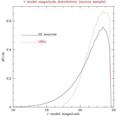
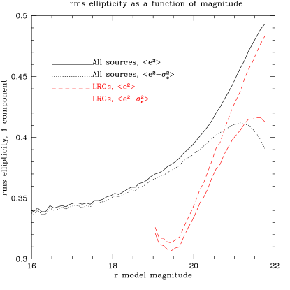
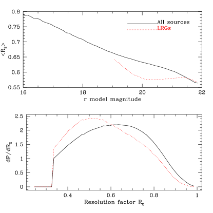
For reference, we include here some plots showing information about the source sample (these plots also show information about the high-redshift Luminous Red Galaxy, or LRG sample, a subsample of the source catalog, that will be described in more detail in §3.4). The magnitude distribution of sources in the catalog is shown in figure 2. The rms ellipticity as a function of magnitude is shown in figure 3. The plot of the average as a function of magnitude, and of the overall distribution of values, is in Fig. 4. Some general information about the catalog is included in table 2. Note that for all tests performed in this paper, we divide the sources into three samples: , , and high-redshift LRGs.
2.2.2 Shear calibration bias
Here, we list the sources of shear calibration bias that were described in detail in H04, and estimate their magnitudes for the source catalog used here; refer to that paper for more detail about estimated shear calibration uncertainty.
There are five major sources of shear calibration bias, as listed in H04. First, we consider the PSF dilution correction, the correction to the measured galaxy image to account for the blurring due to convolution with the PSF. Unlike the linear PSF-correction method using in H04, which has significant shear calibration uncertainty due to this effect for the less well-resolved galaxies, the re-Gaussianization method only has a few per cent shear calibration uncertainty (Hirata & Seljak, 2003) even for the lower limit studied in that paper. For this paper, a plot of the PSF dilution correction as a function of , for both exponential and de Vaucouleurs profiles, for various values of source ellipticity, is shown in Fig. 5.

We model the calibration error due to the PSF dilution correction as due to a sum of contributions from exponential profile and de Vaucouluers profile galaxies,
| (13) |
where and are the weighted fractions of the two types of galaxies with . A lower bound on can be obtained from Fig. 5 by noting that for the exponential profile and for the de Vaucouleurs profile, hence
| (14) |
For the upper bound, we repeat this calculation, except that we use the corresponding to and ellipticity equal to (since this is the rms total ellipticity). This calculation is conservative since most galaxies are at where is less (at fixed ). (We find that and are almost completely uncorrelated after the noise is subtracted from for each of our three samples, and for both the de Vaucouluers and exponential sources within each of these samples.) The results are shown in Table 3; these should be interpreted as bounds, since it is likely that some cancellation between positive and negative dilution galaxies occurs.
| Sample | LRG | ||
|---|---|---|---|
| 0.59 | 0.58 | 0.33 | |
| (exp) | 0.39 | 0.41 | 0.41 |
| (deV) | 0.38 | 0.42 | 0.37 |
| Calibration bias (per cent) | |||
| PSF dilution | |||
| PSF reconstruction | |||
| Selection bias | |||
| Shear responsivity error | |||
| Noise rectification | |||
| Total (per cent) |
Next, we consider errors in PSF reconstruction, which can arise if the PSF ellipticity or trace are misestimated by the Photo PSF pipeline. This error was considered by H04, which showed that the PSF trace is accurately reconstructed to within . We can use Eq. (20) of H04 to estimate the resulting calibration error; we find weighted averages , , and for the , , and LRG samples222The values are the same for the and bands to within for the and samples. For the LRG sample, we find in and in ; we quote the value here because the signal-to-noise ratio for the LRGs is typically greater in and hence this measurement is weighted more heavily. This is certainly conservative as the error increases with increasing . respectively, resulting in calibration errors of (), (), and per cent (LRG).
We also must be concerned about shear selection bias, the preferential selection of galaxies at low or high ellipticity. Considering that figure 3 shows clear evidence for evolution of with magnitude, we do not estimate selection bias using the method from §3.2.3 of H04, which assumes no evolution of rms ellipticity with magnitude. An alternative method of estimating the shear selection bias utilizes a simple model of the selection criteria. This method is not dependent on assumptions about the evolution of the ellipticity distributions. The main selection criterion that can be influenced by shear is the resolution factor cut, which favors highly elongated galaxies, since these have a larger trace after PSF convolution than a circular galaxy with the same area. We model this by noting that for a Gaussian galaxy and PSF, the resolution factor obeys
| (15) |
where and is the ellipticity of the pre-seeing galaxy image. A gravitational shear along the -axis leaves fixed but changes according to
| (16) |
where is the amount of the shear. Therefore the change in resolution factor is
| (17) |
Now the effect of the cutoff on the mean ellipticity can be estimated by averaging the ellipticities of the galaxies that are accepted into the catalog because of the shear (the integrand is negative when galaxies are removed or their ):
| (18) | |||||
where is the position angle333Defined by . and is the joint ellipticity-resolution factor distribution. In the last line we have approximated and as independent, which we have found to be very nearly true, and noted that the mean value of is because the ellipticity has 2 components. The shear calibration error due to selection at the cut, assuming that all galaxies are weighted equally, is
| (19) |
where is the shear responsivity which is discussed further in subsection 2.3. Note that cannot be estimated from Fig. 4 because that plot shows the distribution of values in the -band. For this calculation, the relevant quantity is the distribution of values formed by choosing (for each source) the lower of the two values, since that number is what determines whether the object is included in our catalog. Furthermore, we must use the distribution of values weighted by the weights used in our lensing analysis. For a typical value of for each sample from §2.3, our cut value , and weighted values , 2.4, and 2.8 for the , , and LRG samples, respectively, we obtain a selection bias estimate , 0.103, and 0.111 for , , and LRGs.
However, the cut is not the only one that will cause shear selection bias; the detection requirement that will lead to selection bias in the opposite direction, though the magnitude of the effect is not as great (see Appendix C, which shows the calculation of the estimate as , , and for the three samples respectively). Consequently, we consider the estimate of shear selection bias to be as low as zero and as high as the values estimated only taking into account the selection.
Shear responsivity error is an error in the shear responsivity via a systematic uncertainty in . We use a value of estimated from figure 3, with different results used for the full source catalog and for the high-redshift LRG sample. (Note that in light of our shear selection bias results, we may consider that the increase of with magnitude is in part due to shear selection bias, since the average is lower at fainter magnitudes, and therefore the selection bias should be more severe there. Even if this is true, it is still correct to use the value of when computing the shear responsivity.) We estimate the systematic error in assuming that the uncertainty in is its primary source of uncertainty. To estimate uncertainty in , we looked at the southern galactic survey area, for which there are many repeat observations of the same area (as many as 27 for some areas) that can be used to get empirical values of that can be compared against the theoretical value derived from Eqs. 11 and Eqs. 12. We find that is overestimated by about 0.010 ( confidence interval ), yielding an estimate of shear calibration bias of according to Eq. 25 in H04.
The final major source of shear calibration bias is noise-rectification bias, whereby the noise in the image leads to a bias in the ellipticity due to the non-linearity of the PSF correction process. As shown in H04, equation 26–27 and Appendix C, the noise-rectification bias can be estimated as
| (20) |
where is the signal to noise of the detection averaged over bands:
| (21) |
For high- galaxies, , decreasing to for and then increasing to at our (and rising rapidly at lower , as high as for ). For each source sample, we compute the weighted average value of , to find noise-rectification bias of (), (), and (LRG). To estimate the error, we consider the allowed range of the noise-rectification bias to be equal to the magnitude of the error estimated above; results are shown in table 3.
Those five effects are the major sources of shear calibration bias; there are also several minor sources, at the 0.1 per cent level. These include camera shear (for which we correct using the astrometric solutions, as described in §2.2.1), errors due to pixelization, and atmospheric refraction effects. We do not attempt to estimate values for these subdominant sources of error. The total shear calibration bias (at the level) with the five main sources of error taken into account is shown at the bottom of table 3 for the three source samples individually. These estimates are conservative in that they do not assume any distribution for these errors, allowing the actual values to add, rather than adding them in quadrature (which assumes some possible cancellation).
2.3 Shear estimator
The weighting used for this work differs from that of H04 in two ways. First, rather than the uniform weighting used in that paper, we weight by measurement error:
| (22) |
where , the rms shape noise in one ellipticity component, was determined as a function of model magnitude from Fig. 3 for the full source catalog and LRGs separately, and is the error per component on the ellipticity from equation 11. This weight is then multiplied by , downweighting lower redshift lenses and lens-source pairs with small redshift separation relative to those at large separation. Consequently, the weight used for a given pair is . The shear responsivity appropriate for this weighting scheme is then computed using equations (5-33) and (5-35) from Bernstein & Jarvis (2002), with the average value for our source samples being 0.86 for the sources, 0.83 for the sources, and 0.85 for LRGs.
Using these weights, the shear estimator is then
| (23) |
While we also tried an ellipticity-dependent weight as suggested in Bernstein & Jarvis (2002) to increase signal-to-noise, we found it had minimal effect on the errorbars, so all the work in this paper was done with the weighting scheme described above.
2.4 Error determination
Several methods of determining the errors on were used, each with its own advantages and shortcomings. We describe them here, and in §6.2 we compare the results in order to determine on which to rely.
2.4.1 Analytic computation
Analytic expressions for for a given weight function may be derived from equation (5-27) in Bernstein & Jarvis (2002). This method is the least computationally expensive method of deriving errors, but suffers from several shortcomings. First, it gives incorrect results in the presence of spurious shear power in the source catalog. Second, it does not allow an easy way to include errors on the boost factors, which may be significant. Finally, it does not account for correlation of radial bins, which can be significant at large radius, where the average lens-source separation is larger than the average lens-lens separation, so a given source contributes to the measurement in several radial bins.
2.4.2 Random catalogs
A more computationally expensive way of determining the errors is using random lens catalogs. In the absence of systematic shear, the average signal around random points should be zero, and the rms deviation around the mean gives some measure of the noisiness of the signal, and therefore of the errors when using the real lens catalog. However, as described in H04, this method is only valid on small distance scales, less than about 500 kpc for the faint lens samples and around 1 Mpc for the brighter samples. Furthermore, this method also cannot take into account the errors on the boost factors, though it can account for the correlation of radial bins. To get a reasonably smooth measure of the errors, a large number of random catalogs must be used; for this work, we used 24.
2.4.3 Bootstrap resampling
As described in H04, bootstrap resampling is a useful method of determining the errors. For this purpose, the lens catalog is divided up into 200 subregions, and the signal is computed for each subregion. The bootstrap-resampled datasets are generated by combining the signal from 200 subregions with replacement. Then, a large number of resamplings (for this work, 2500) can be used to determine the average signal and its error. This method has several advantages over the other two; for example, it naturally incorporates errors in the boost factor, and the correlation of radial bins. However, because of the finite size of the subregions, the errors are once again not trustworthy at large lens-source separation. Also, as described in H04, the noise in the covariance matrix means that the values for fits performed using the covariance matrix do not follow a distribution.
3 Redshift distributions
In this section, we first describe the many commonly-used methods of source redshift determination, including potential errors. Then, we describe the “reference” redshift distributions that we use for calibration.
3.1 Photometric redshifts
Surveys that collect photometric information in several passbands allow for the determination of photometric redshifts, which use the galaxy colors to extract an approximate redshift, typically based on the construction of galaxy spectral energy distribution (SED) templates that are evolved with redshift. In principle, these photometric redshifts may be used directly in the computation of . To be accurate, this computation should take into account the photometric redshift error distribution, which may be highly non-Gaussian, particularly in certain redshift ranges and areas of color space.
We studied photometric redshifts computed by two independent groups for the SDSS, and found that they performed statistically nearly identically (that is, photometric redshifts for particular galaxies were not necessarily the same, but the mean bias and scatter were nearly the same as a function of magnitude and of photometric redshift). One set of photometric redshifts was computed using the program kphotoz as mentioned in §2.2. The other set was computed by the SDSS photometric redshift working group (as discussed in Csabai et al. 2003, based on work in Csabai et al. 2000 and Budavári et al. 2000), for DR1 data only. Because of the lack of photometric redshifts for the full DR2 sample, instead of using the nearest-neighbor search method from H04 to get photometric redshifts for the full sample, we demonstrate results in this paper using redshifts from kphotoz for the full sample.
We only use photometric redshifts for sources at , because of the large scatter at fainter magnitudes that will be demonstrated in §6.1.2. The mean redshift of the source sample at is 0.35, with a fairly large width. This fact raises several concerns for use with the lens sample, which extends out towards the peak of this redshift distribution at the bright end. Lenses at higher redshift are weighted more highly because of their higher , so that if many of the lens-source pairs are at small redshift separation, and there is a bias on the photometric redshifts, then even with the weighting which downweights nearby pairs, we still end up with a large bias in . Consequently, the photometric redshift error distribution, which can be difficult to determine, is very important. Previous studies used the spectroscopic sample, which is brighter, with much lower photometric errors, supplemented by the CNOC2 spectroscopic redshifts down to (Csabai et al., 2003), or used stacked images from the southern SDSS survey due to their lower photometric errors (for kphotoz444Michael Blanton, private communication.). Consequently, the applicability of the photometric redshift errors from these studies to a full catalog based on fainter single images (that will have additional photometric redshift error due to noise) is questionable.
Fortunately, as will be shown in §3.3, we now have the capability of studying the errors in photometric redshifts directly for a representative subsection of our source sample rather than for atypical brighter or noiseless samples, and the application of these error distributions in the computation of the lensing signal can help eliminate the bias in due to photometric redshift error.
3.2 COMBO-17 distribution
Another commonly-used option for the source redshifts is the use of a probability distribution rather than individual redshifts. This method has the disadvantage of leading to a larger boost factor due to the inability to weed out physically associated pairs. However, for the galaxies, distributions are a better option than photometric redshifts due to photometric noise; consequently, we do not consider photometric redshifts for .
The redshift distribution used for this paper is derived from data from the Classifying Objects by Medium-Band Observations, or COMBO-17 survey. COMBO-17 includes photometry in 17 passbands spanning the wavelength range from 350–930 nm, yielding far more information for the determination of photometric redshifts than the SDSS. The area of the survey used in the study that derived the redshift distribution covers 0.78 square degrees, spread over three disjoint regions (smaller than the full survey), so while the area is small, the concern about the derived redshift distribution being unduly influenced by large-scale structure is somewhat lessened. Wolf et al. (2003) includes the luminosity functions upon which these distributions were based. Since the distributions are for all photometric galaxies rather than those passing our lensing cuts, we may expect that they lie at slightly higher redshift than our catalog on average; we show results of tests of this hypothesis in §6.4.2. A plot of this distribution (averaged over ) is shown in comparison with other distributions in Fig. 7.
3.3 DEEP2
Another way to determine the true redshift distribution for our sources is to find another survey that is flux-limited and complete to a desired flux. As shown in Ishak & Hirata (2005) in the context of cosmic shear surveys, even just 100 spectroscopic redshifts may be sufficient to make this determination. Fortunately, the DEEP2 survey (Davis et al. 2003, Madgwick et al. 2003, Davis et al. 2004, Coil et al. 2004a) provides results that are useful for this purpose, with spectroscopic completeness well beyond , the limits of our source catalog. The DEEP2 survey will eventually include spectroscopy of 60 000 galaxies in 4 fields totaling 3.5 square degrees. While the targeting in three fields involves the use of photometric information to select galaxies with , the targeting in the extended Groth strip (EGS) does not attempt to place such restrictions, and because it overlaps with the SDSS, it may be used to study redshift distributions and photometric errors in SDSS data. Observations are complete in pointing one of field one (EGS), centred at Dec. and RA , which has area approximately 0.15 deg2 (roughly the area in the full EGS). The Groth strip is situated degrees from the nearest of the three COMBO-17 fields, so the redshift distribution obtained from it can be considered statistically independent from the COMBO-17 results. The detectors on the Canada-France-Hawaii Telescope (used for imaging for DEEP2 target selection) saturate at at the bright end, so no galaxies brighter than that limit have spectra, but fortunately those galaxies constitute a very small fraction ( per cent) of the source sample. Also, about 1/3 of the galaxies in the Groth strip were not targeted at all, which reduces the number of potential matches against SDSS.
The target selection in the Groth strip did involve some color and magnitude information (Faber et al., 2005). At , all galaxies are selected uniformly; fortunately, the majority of the galaxies in our lensing catalog fall into this category. At fainter , galaxies are classified as low or high redshift via color cuts; low redshift galaxies are downweighted significantly, which makes the selection fairly complicated. To verify that this selection has a negligible effect on the results in this paper, all redshift distributions computed using DEEP2 data were recomputed taking into account selection probability (i.e., weighting each redshift by ). The value of for various values of lens redshift and with the weighted redshift distributions were computed and compared to the values from the unweighted distributions. Even for lens redshift , which is at the high end of the distribution, and should be more sensitive to the source redshift distributions than most other lenses, the fractional change in the value of was on the order of a few tenths of a per cent. Consequently, we consider the selection function to be of negligible importance for the distributions presented in this paper, and for the remainder of this work we use the unweighted results.
To use the DEEP2 redshifts to compute redshift distributions and photometric redshift error distributions for our catalog, we first matched between the DEEP2 spectroscopic catalog in the Groth strip and our lensing catalog. This step ensures that all distributions that we derive will apply to lensing-selected galaxies, which are expected to be at lower average redshift than all galaxies at the same magnitude, due to our requirements on the shape measurement. In principle we could have used redshift distributions as a function of magnitude presented in Coil et al. (2004b), but since those were derived for all galaxies, they are expected to be at slightly higher average redshift than the distributions for lensing-selected galaxies. Once matching was complete, there were 278 matches, 162 at and 116 at . Our requirement that there be a high-quality redshift had eliminated 33 potential matches, giving a redshift determination success rate of 89 per cent for lensing-selected galaxies overall, or 91 per cent for and 86 per cent for .
We must be concerned about the effects of redshift failures on our results. The lack of knowledge whether or not the failures lie in a particular region of redshift space (e.g. higher redshift on average) introduces an unknown systematic into our results. First, we note that as discussed in Coil et al. (2004a), redshifts cannot be measured by the DEEP2 survey. However, for the magnitude ranges of interest in this paper, this limit is effectively of no importance. Second, we find that the fraction of matches with failed redshift determination varies somewhat with magnitude (6 per cent failed at , 8 per cent at , 11 per cent at , and 14 per cent at ), implying an increase in failures at higher redshift; we may also have a problem if the majority of the failures lie at a particular part of the redshift distribution in a given magnitude range. We can place bounds on the effect of such a systematic as follows: we compute the change in that results from assuming that all the failed redshifts were at 0 and at (which yields the asymptotic value of ). We can compute the fractional error
| (24) |
where is the fraction of redshift failures (0.11), is the average value of for those galaxies that had failed redshift determination, and is the average value of for those galaxies that were used to compute the signal using the observed redshift distribution. If we assume all failed redshifts were 0, then , and therefore we expect a bias of -11 per cent (or per cent for and per cent for ), where our use of the redshift distribution from the redshift determination successes overestimated (and therefore underestimated the signal) by that amount. If we assume all failed redshifts are , then the effect depends on the lens luminosity (where it is less important for lower luminosity and redshift lenses, for which all sources were essentially at anyway) and the source sample. The degree to which the signal was overestimated in this case is given, for each luminosity bin and source sample, in table 4. As shown, the effect is at most 2.7 per cent overestimation for L6 with sources, much less for the faint bins. The reality is somewhere in between these two extremes, most likely towards the higher end of the range quoted since we expect more redshift failures at higher redshift, but cannot easily be estimated, so we use these values to define the 95 per cent confidence interval. (This estimate did not take into account the effect of changes in on the weighting, since the use of non-optimal weighting should increase the errors without inducing a bias.)
| Lens sample | , per cent | |
| L1 | 0.1 | 0.4 |
| L2 | 0.2 | 0.6 |
| L3 | 0.5 | 0.9 |
| L4 | 0.9 | 1.4 |
| L5 | 1.6 | 1.9 |
| L6 | 2.7 | 2.5 |
We compared the magnitude distribution among the matches to that in our source catalog. If they are not comparable, redshift distributions determined using the DEEP2 sample may not be applicable to our source sample. Table 5 shows a comparison of the samples. The first column shows the fractions of galaxies in magnitude bins for our source catalog overall, and the second column shows the fractions in the Groth strip (with 95 per cent confidence intervals from the binomial distribution for the latter due to its small size). Since they agree within the errorbars, we need not worry about the Groth strip being very different from the full source catalog. The third column shows the fractions in magnitude bins for the full SDSS photometric sample (i.e. no lensing-related cuts), Groth strip only, restricted to the magnitude range for which the CFHT detector does not saturate. The fourth column shows the fractions of galaxies actually targeted as a function of magnitude (for ); this column is statistically consistent with the third column, implying that the targeting is indeed independent of the magnitude. Finally, the fifth column shows the fractions of galaxies as a function of magnitude for the matches between the DEEP2 redshift catalog and our lensing catalog with successful redshift determination, which is consistent with column two, the fraction of lensing-selected galaxies as a function of magnitude in the Groth strip before matching against DEEP2, with the exception that the DEEP2 galaxies are by necessity missing the sample, which is roughly 2 per cent of our catalog. Furthermore, the fraction of galaxies categorized as high-redshift LRGs was similar in the two samples (9 per cent in our background catalog, versus per cent in the DEEP2 matches at the 95 per cent confidence level), implying that there is no color-dependence of the targeting and redshift failures with regards to this particular subsample.
| Magnitude | Lensing | Lensing catalog, | Photometric survey, | DEEP2 | DEEP2 |
|---|---|---|---|---|---|
| range | catalog | Groth strip | Groth strip | targets | matches |
| 0.022 | 0.000 | 0.000 | 0.000 | ||
| 0.055 | |||||
| 0.153 | |||||
| 0.358 | |||||
| 0.411 |
While using the spectroscopic redshift distributions may seem to be the ideal way of determining , there are two caveats that make this solution less promising. First, the use of average redshift distributions without any use of photometric redshift errors means that many more physically-associated lens-source pairs are included in the calculation. While the resulting dilution of signal may be corrected for using boost factors, boosting is another potential source of systematic error since we cannot correct for intrinsic shear, and it is desirable that the boost factors be as low as possible. Second, because these distributions were determined using a small portion of the sky, they may be unduly influenced by large-scale structure, and not representative of the redshift distribution in the survey as a whole (in §6.1, we show how the effects of large-scale structure increase the errorbars determined purely using statistics). The ideal solution to the second problem would be to have spectroscopic redshifts determined for a random sample of galaxies selected from the entire SDSS survey area, which could be used to determine source redshift distributions or photometric redshift error distributions.
Consequently, we also used these DEEP2 redshifts to determine photometric redshift error distributions, enabling us to use photometric redshift information to eliminate physically-associated pairs, yet to also avoid any bias due to errors in the photometric redshifts. The determination of these error distributions was done by dividing the matches into bins based on photometric redshift (in order to determine error distributions as a function of photometric redshift). Our computation of then takes into account the photometric redshift error distribution:
| (25) |
The signal is then computed as usual, but instead of assuming that (i.e., ), we use the value computed by evaluating the integral in equation 25.
Results from our work with the DEEP2 data are shown in §6.1.
3.4 Reference distribution: LRGs
There is one subset of SDSS source galaxies for which excellent redshift information is known: Luminous Red Galaxies (LRGs) (Eisenstein et al., 2001). These galaxies have a well-known color-redshift relation that allows photometric redshifts to be determined with excellent precision.
For the LRGs selected according to criteria shown below, the photometric redshifts perform significantly better than for the general source sample. Furthermore, as shown in Padmanabhan et al. 2004, redshift distributions for LRGs from the 2dF-Sloan LRG and Quasar Survey (2SLAQ) can be used to construct very reliable redshift distributions for these galaxies. Note that for LRGs, the redshifts used were from a simple template code discussed in Padmanabhan et al. (2004) rather than from kphotoz; however, for most regions of color space occupied by LRGs, the results are highly correlated.
The selection criteria used for the LRGs are as follows:
-
1.
-
2.
-
3.
-
4.
-
5.
-
6.
These criteria were chosen as the combination of those from Eisenstein et al. (2001) and from Padmanabhan et al. (2004) that best suited the requirements of this work, namely very low levels of contamination from non-LRGs, from low-redshift LRGs, and from stars, yet sufficient numbers that the LRG sample can be used as sources for weak lensing with reasonable signal to noise.
Imposing these criteria on our source catalog yields 2 884 242 LRGs total, though only about 65 per cent are in regions with lenses. A plot of the LRG redshift distribution derived using 2SLAQ work (Padmanabhan et al. 2004) is in Fig. 6; for this distribution, only the 72 per cent of the LRG sample with photometric redshift greater than 0.45 were used because the inversion method gave unreliable results for . As shown, the redshift distribution peaks around , which illustrates another advantage of using LRGs as sources: when we use SDSS main spectroscopic sample galaxies as lenses, with redshifts mostly below , does not vary strongly with source redshift for sources at such high redshift, so an error in these distributions will make a very small difference in the results.

Note that approximately 57 per cent of the LRGs in the catalog are fainter than model magnitude of 20. Padmanabhan et al. (2004) only includes redshift distributions down to this limit, so our use of that inversion method for this sample is suspect. However, tests of photometric redshifts using the DEEP2 matches indicate that that the mean bias is the same for the LRGs as for the LRGs (0.02), and the rms scatter is larger but not excessively so (0.07 vs. 0.05), which suggests that the use of the inversion method in Padmanabhan et al. (2004) with the same error distributions for and is justified here.
In addition to computing the signal with the full sample using the photometric redshifts directly, and with the restricted sample using the redshift distribution, we also computed it with photometric redshifts on two subsamples, those with and . Because these stricter cuts would help avoid contamination by lower-redshift galaxies being scattered up to higher redshift, we try imposing them on our sample; if the signal does not differ when we do this, then we know that using the full sample is relatively safe.
Fig. 2 shows the model magnitude distribution of sources classified as high-redshift LRGs, and Fig. 4 shows their distribution, in comparison to the values for the overall source sample. As shown, the LRG sample is, on average, at lower and fainter magnitudes than the other source samples, and thus we may be concerned that it will have more significant shear calibration bias, as evidenced by the confidence intervals in Table 3.
In principle, given the excellent redshift information for the high-redshift LRGs, one solution to our lack of reliable redshifts for all sources would be to do g-g lensing entirely with LRGs as sources. However, we then are faced with a problem of statistics, since LRGs are such a small fraction of the sources available (9 per cent), yielding large statistical errors on . This problem is the reason why our test for calibration bias is so useful; it allows us to use the excellent redshift information from LRGs to check the calibration of the lower-redshift source samples, which contain many more galaxies, enough to obtain excellent statistical errorbars.
4 Other Systematics Issues
Here we consider a number of remaining systematics issues that arise when computing the lensing signal. Some are calibration uncertainties that scale with the signal, similar to the shear and redshift distribution calibration uncertainties discussed previously; others are systematics that do not scale with the signal, and have amplitudes that depend on the angular or physical lens-source separation.
4.1 Random points test
The random points test requires computing signal using random lens catalogs (i.e., sets of random positions generated with the angular mask of the spectroscopic survey area, using the same lens redshift and magnitude distributions as the real lens sample). In practice, these distributions are preserved by drawing the redshifts and magnitudes from the real sample, without replacement. The random points test is useful because a nonzero signal reveals the presence of spurious shear power (systematic shear) in the source catalog which would lead to an additive bias in the lensing signal. The random catalogs used for this work were generated using mangle (Hamilton & Tegmark, 2004).
In the absence of systematic shear, we expect the random points test to show zero signal around random points. However, there is a slight smearing of images in the scan direction because the charge transfer is not continuous, instead occurring in very quick transfers from pixel to pixel, so that the PSF is convolved with a rectangle one pixel (0.4”) wide along the scan direction only. The result is that the PSF is not circularly symmetric. This effect may be exacerbated if the scan rate and charge transfer rate are not perfectly matched, leading to convolution on a scale larger than one pixel.555We thank James Gunn for pointing out this effect. While in principle PSF-correction algorithms should correct for PSF asymmetry, in practice this is difficult to do perfectly. In addition, since the charge-transfer efficiency may also depend on the amount of charge, the PSF asymmetry may be different for faint objects than for bright ones, but since Photo fits the PSF using stars around , code that uses the Photo PSF may not be able to fully correct for this effect. We found that the re-Gaussianization scheme over-compensates for the effect.
We address the presence of this spurious signal by determining it to as high precision as possible using random catalogs (where the number of random catalogs is limited by processor time), then subtracting it from the observed signal. This procedure results in the errorbars on the signal rising by a factor of . Our choice of means that the errorbars only increase by 2.1 per cent. Results for the random catalog test are shown in §6.3.
However, random catalog signal subtraction, while widely accepted in the literature, ignores the possibility that fluctuations in the number density and systematic shear may be correlated. We describe this problem as follows: A g-g weak lensing measurement entails computing the correlation . The measured number density of lenses can be decomposed into , an average density of sources on the sky plus fluctuations. The measured total shear can be decomposed into , the true shear field plus systematic shear. When we compute the signal around random points, we obtain the quantity . Random catalog subtraction thus corresponds to measuring
| (26) |
The first term on the right side, , is the correlation that we hope to measure, but the second term is an additive systematic error that has not been discussed in previous works on g-g weak lensing. We cannot assume that and are completely uncorrelated, because both quantities are slightly correlated in some way with the PSF. There are several ways in which such an effect could become significant. For example, since there is a gap between camcols on the SDSS camera, the same region must be rescanned with some offset to fill in that gap on a different night, which may have very different seeing and other conditions, such that fluctuates on small scales. If the number density of lenses also fluctuates on the same scale, then we could have some nonzero contribution from the term. For this work, we assume that this term is negligible, since the correlation should be small and has never been detected before, but this issue should be addressed more fully in future work to ensure that this assumption is reasonable.
4.2 45-degree test
Another useful test of systematics in the lensing signal is the 45-degree test, which requires computing the lensing signal with the coordinate system rotated by 45 degrees. By inversion symmetry, the 45-degree rotated signal should vanish, with weak lensing only contributing to the tangential shear, . The presence of such a signal could indicate a variety of shear systematic errors, since they generally contribute both to and . We computed the 45-degree rotated signal for all three source samples, so that together these tests were done for all sources in the catalog (we assume that the choice of redshift distribution does not matter for this test, as would be nonzero due to shear systematics, so we only use one choice of redshift determination method for each of those samples). Results for this test are in §6.3.
4.3 Star-galaxy separation
Star-galaxy separation is an important issue for weak lensing, since the inclusion of stars in the source sample would dilute the signal. Thus, a balance must be struck, ensuring the purity of the galaxy sample used as sources, while avoiding being overly conservative and eliminating too many galaxies in the course of doing this separation (which would lead to poor statistics). Star-galaxy separation for this catalog was accomplished via two cuts: first, the requirement that the Photo flag OBJC_TYPE be equal to 3, or galaxy; and second, the requirement that (i.e., the object must be 50 per cent larger than the PSF). The type determination for DR1 and DR2 is described in Lupton et al. (2001); in brief, it utilizes the linear combination of fits of galaxy profiles to two models (exponential and de Vaucouleurs), then allows the ratio of the flux in a fit to a PSF shape to that in the linear combination of galaxy models to determine the type, via the requirement that for galaxies. As shown in figure 3 in that paper, this procedure ensures a relatively pure galaxy sample even close to , with stellar contamination fraction (determined using Hubble Space Telescope, or HST data in the Groth strip) being negligible at brighter than 21, and 7 per cent for . It is also clear from that figure that OBJC_TYPE is much more likely to default to calling galaxies to stars rather than vice versa, with galaxy contamination of per cent in a sample of “stars” for . While there are probabilistic methods that are more accurate at the faint end (), such as that used in Scranton et al. (2002) and Sheldon et al. (2004), OBJC_TYPE’s conservative tendency should not cause significant stellar contamination, though it does reduce the density of sources in poor seeing at faint magnitudes.
In order to check that our shape measurement cuts reduce stellar contamination due to failures in OBJC_TYPE, we used publicly-available catalogs from the Great Observatories Origins Deep Survey (GOODS), carried out via the HST (Giavalisco et al. 2005, Giavalisco et al. 2004). Characterizations of stars versus galaxies are much more accurate to fainter magnitudes in space-based surveys such as this because the PSF is much smaller. We found 577 objects at (of which 60% are at ) that were matches between the full SDSS photometric catalog and the GOODS north field, centred at Dec. and RA . We found that the “galaxy” classification is incorrect about 1.5 per cent of the time for and 7 per cent of the time for objects, and the “star” classification is incorrect a larger fraction of the time (3 per cent at and 40 per cent at ), confirming the results from Lupton et al. (2001) that OBJC_TYPE tends to default to calling small, faint objects stars.
However, when we restrict to the subset of 146 objects that passed all shape-measurement and other criteria to be included in our source catalog, of which 73 are at and 73 at , we find that only 2 (1.4 per cent) of those included are stars, or 0 per cent contamination in the sample and 2.7 per cent contamination in the sample. We see that the resolution-factor and other cuts reduce stellar contamination by a factor of three from the result using OBJC_TYPE alone. Using the binomial distribution to get 95 per cent confidence intervals on out stellar contamination estimates yields () and (). Technically, we should take into account that the GOODS north field is at , but the average value for the full lens sample is , so we might expect slightly higher stellar contamination in the full catalog than that computed for the GOODS field. However, because the dependence of stellar contamination on is difficult to model, we do not attempt any correction.
To check the signal for contamination of our source catalog by stars, we computed the signal at low versus at high galactic latitude (cutting at ) to compare the results. Note that while finding a lower signal at low galactic latitude may indicate a problem with star/galaxy separation, it may also indicate the presence of other systematics. In particular, since the extinction is greater at low galactic latitudes, galaxies near the faint end at a given magnitude were actually lower signal-to-noise measurements at low galactic latitude than they were for high galactic latitude, so in principle there could be a shear systematic causing a difference between these two samples as well. The results of this test will be shown in §6.3.
4.4 Seeing dependence of calibration
Because our ability to correct the galaxy image for effects due to the PSF depends on the relative size of the galaxy and the PSF, we must consider the possibility of a seeing-dependent shear systematic. Consequently, for each galaxy, we consider the size of the PSF used, and split our sample into “good seeing” (PSF size less than the median value, 1.25 pixels in the band) and “bad seeing” (PSF size greater than the median value). The signal was then computed using these two source samples, and compared. Results for this test will be shown in §6.3.
4.5 dependence of calibration
Because some calibration biases may be more prominent at lower , it is important to check for -dependence of the calibration. There are several effects that could lead to apparent dependence of the calibration: noise rectification bias, selection biases, and biases due to PSF-correction, which would be particularly important for less-well resolved galaxies. We computed signal using sources with greater than and less than 0.55 in each band to check for bias; results of this test are presented in §6.3.
4.6 Systematic differences between bands
Like many other studies, we used shape measurements averaged over two bands, the and bands. While the shape measurements between the two bands may legitimately differ for individual objects, due to (for example) spectral differences in emissions from the disk versus from the bulge of spiral galaxies, we also checked to ensure that the signal computed with the shape measurements from each band individually gives the same . The results of this test will be shown in §6.3.
4.7 Boosts
As discussed in H04, the lensing signal at small transverse separations is diluted by the inclusion of sources that are physically associated with the lens (i.e., are in the same group or cluster), and therefore are not really lensed. To correct for this effect, the signal for a given luminosity bin is boosted according to the weighted number of galaxies per unit area relative to the number from random catalogs. The signal is multiplied by a factor
| (27) |
where is the weighted number of galaxies per unit area when the signal is computed, and is the same computed with random lens catalogs. The number from random catalogs takes into account the decrease in the number per area with radius due to survey edge effects, so the boost can accurately account for the dilution of signal by physically associated pairs. Consequently, is the lens-source correlation function.
The boosts add two sources of statistical error and two sources of systematic error. In the rest of this section we consider each of these.
4.7.1 Statistical errors
The statistical error arises because the boost factor is the ratio of two noisy quantities, and . The noise in can be minimized by computing signal from a large number of random catalogs, where 24 are used for this work. However, for subsamples with a small number of lenses, is still slightly noisy at small separations due to the small size of the radial bins; this noise is taken into account in the bootstrap by multiplying the boost from each dataset and radial bin by a Gaussian random number of mean 1 and standard deviation equal to the fractional error in as computed from the random catalogs. The noise in is taken into account naturally by the bootstrap, since each bootstrap resampled dataset will have a slightly different used for the boost. Hence, the statistical error due to the boosts is simple to take into account.
4.7.2 Systematic error: non-uniformity of boost factor
One potential systematic error arises because both and the boost factor vary strongly with luminosity at the bright end of the lens sample, so the luminosity bins that are 1 magnitude wide may be too wide to properly compute the signal in the innermost radial bins, kpc, where the boost is most important. By averaging over a large range in luminosity, with and varying with luminosity, we may run into a situation where the product of two averages ( and separately averaged over luminosity, then multiplied) differs significantly from what we really want, the average of products ( averaged over luminosity).
One rudimentary method of detecting the effects of using wide luminosity bins on the boost factor is to split the brightest luminosity bin in half, compute the signal separately for each half (boosting each one individually), then average the signal from each half. The resulting signal can be compared against the signal computed using the full luminosity bin. Results for this test will be presented in §6.3.
4.7.3 Systematic error: magnification bias
Another boost-related source of error is magnification bias, since the number of galaxies per area around real lenses may not be expected to be the same as that around the random points. There are three competing effects: first, that due to the magnification (in the weak lensing limit), where , the number of lens-source pairs per unit area on the sky will decrease; second, that the magnification means that fainter sources will be visible than would have been otherwise, and therefore the number of lens-source pairs per unit area will increase; and third, the magnification changes the resolution factors of the source galaxies. The competition between the first two effects can be quantified by , where is the total number density of source galaxies given a faint magnitude limit of . For the sample, we must taken into account the loss of sources at the bright magnitude limit of 21, and compute
| (28) |
where is the faint magnitude limit and is the bright magnitude limit. We compute separately for each source sample: for the source sample, we find ; for , we find (i.e. when the magnitudes are shifted brighter, we lose more galaxies at the bright end than we gain at the faint end because of our cuts on the shape measurement); and for the LRG sample, we find .
The resolution factor dependence of this effect has not been previously evaluated. If we take the Gaussian approximation for the galaxy, , and note that in the weak lensing regime, we find that the effect of magnification is to adjust the resolution factor by
| (29) |
The number of galaxies that are gained due to the resolution factor cut is then
| (30) |
where is the resolution factor distribution normalized to . The total change in the number density of galaxies is then
| (31) |
For the three source samples, using the values of given above and from §2.2.2, we estimate , , and for , , and LRG samples, respectively. (Without taking into account the effect of the change in , we would have had , , and , so this effect significantly changes our sensitivity to magnification bias.)
The convergence can be simply estimated for roughly power-law profiles as
| (32) |
where represents the mass-sheet degeneracy. We will ignore this since our boost factors approach unity at large separations. Since for our galaxies we find , it then follows that . We can then use computed values of and to estimate . Table 6 shows the best-fit power-law and our resulting predictions for for L3–L6; L1 and L2 are not used because the shear is statistically consistent with zero in these bins, and therefore so is .
| Lens | ||||
|---|---|---|---|---|
| sample | (30 kpc) | (100 kpc) | ||
| without LRGs | ||||
| L3 | 0.68 | 0.011 | 0.005 | |
| L4 | 0.88 | 0.020 | 0.007 | |
| L5 | 1.00 | 0.050 | 0.015 | |
| L6 | 0.95 | 0.15 | 0.049 | |
| L3 | 0.47 | 0.004 | 0.002 | |
| L4 | 0.81 | 0.006 | 0.002 | |
| L5 | 0.92 | 0.016 | 0.005 | |
| L6 | 0.85 | 0.055 | 0.020 | |
| LRGs | ||||
| L3 | 0.70 | 0.019 | 0.008 | |
| L4 | 0.93 | 0.036 | 0.012 | |
| L5 | 0.95 | 0.095 | 0.030 | |
| L6 | 0.89 | 0.31 | 0.11 | |
This effect is not taken into account explicitly, and therefore may lead to a systematic bias in the signal, since we assume that the increase in sources around lenses is due to physically associated pairs. For all samples, we may be overestimating the boosts and therefore (particularly for LRGs). We do not, however, attempt to correct for this attempt explicitly, since until a concrete detection is made, these estimates should not be treated as certain. For the confidence intervals, we use the estimates in table 6 as the expected value, with an expected uncertainty equal to half the magnitude of the estimate.
4.8 Intrinsic Alignments
Satellite galaxies that are physically associated with a lens will not be lensed; however, it is often difficult to remove them from the source sample in the absence of good redshift information, which is why we must use the boost factors described in the previous section. If the satellites are actually aligned with the lens in some way (radially or tangentially elongated), this alignment will cause a false lensing signal. This effect is well-motivated theoretically (Lee & Pen 2001; Hui & Zhang 2002), and there are several claimed detections in the literature of correlations between the galaxy density (or specific features thereof, such as the Supergalactic Plane) and intrinsic ellipticities (e.g. Flin & Godlowski 1989; Lee & Pen 2002; Navarro et al. 2004). We use to represent the signal due to intrinsic shear, which is the shear signal that would be computed using our shear estimator with a population of physically associated galaxies. Note that the galaxy density-shear correlation that concerns us is distinct from the intrinsic shear-shear correlations that add spurious power to cosmic shear surveys (Croft & Metzler 2000; Heavens et al. 2000; Lee & Pen 2000; Catelan et al. 2001; Crittenden et al. 2001; Jing 2002).
In order to place upper limits on contamination due to intrinsic shear, we must determine what fraction of the lens-source pairs are physically associated, and the typical intrinsic tangential shear of these sources. To compute , we use our results for . Limits on (or on the intrinsic ellipticity or position angle) have been obtained by Lee & Pen (2001), Bernstein & Norberg (2002) and H04; we use the results from H04 as these are the tightest constraints on relevant scales. Results for this estimation will be shown in §6.3.8.
4.9 Correction for non-volume limited lens sample
In this section, we describe the corrections that account for the fact that the lens samples are not volume limited, when comparing between different source subsamples. These corrections required us to compute the mean weighted luminosity for each lens-source sample combination. This computation was done as a function of transverse separation in order to check for any systematic effects.
We found that there is a slight variation in the mean weighted luminosity with transverse separation, because brighter lenses are more clustered, so in the regions where physically-associated pairs are abundant (i.e., where ), the mean weighted luminosity of the sample was higher than at larger radii where . We see the same trend in the mean weighted redshift of the sample, as well. However, this effect does not really mean that the mean weighted redshift or luminosity corresponding to the computed signal is larger at small radii, since the excess pairs around the brighter lenses that cause this effect do not contribute to the signal.
We also expect that and may increase at large , because for more nearby (less luminous) lenses, the same transverse separation corresponds to a larger angular scale, and therefore survey edge effects may cause nearby lenses to lose pairs faster than distant lenses. The observation of such an effect would indicate a problematic selection effect, but fortunately we do not see it at the maximum transverse separations studied in this paper (2 Mpc).
The correction when comparing at slightly different is as follows: we use the results of the signal averaged over radius in each luminosity bin to derive a relation . Then, when we compare signals at two slightly different luminosities (typical differences are less than 1 per cent) and , we assume that rather than being 1, the ratio of the two signals should be
| (33) |
If this correction is non-trivial compared to the statistical error, then we must apply it; otherwise, we do not.
5 Application of the systematic test
In this section, we describe our test to determine the effects of the redshift distributions and systematic errors described in §3 and §4, and show calculations justifying our assertion that cosmology plays a negligible role.
5.1 Methodology
First, in order to compute bootstrap errors on the results, we divide our lens catalog into 200 bootstrap subsamples as described in §2.4.3. For each lens luminosity bin and source sample, we compute the signal in each of the bootstrap subsamples, using 46 logarithmically spaced radial bins from 20 to 2000 kpc in order to measure more sensitively where it varies the most, at small transverse separation. (Plots of signal shown in this paper will have many radial bins averaged at small so they are easier to read.)
Next, to account for physically associated pairs and systematic shear, we used random lens catalogs to compute and . Twenty-four random catalogs were used, so that these functions were determined reasonably smoothly.
After this procedure, we performed bootstrap resampling, generating 2500 datasets for each lens luminosity bin and source sample as follows (to avoid confusion, we use Roman letters to denote lens luminosity bins and Greek letters to denote source samples):
-
1.
For each lens-source sample combination, we use the same set (in order to take into account correlations) of random numbers drawn from a uniform distribution to choose 200 bootstrap subsamples randomly, with replacement. The signal from these subsamples are then averaged to get signal for each of the lens-source sample combinations, .
-
2.
We compute boost factors using the weighted number of pairs per unit area relative to the average weighted number from random catalogs . The error in is taken into account by the bootstrap procedure itself, and the error in is taken into account via multiplication by a Gaussian random number of mean 1 and standard deviation equal to the fractional uncertainty in , where a different random number is used for each , , and radial bin.
-
3.
We use the measured random catalog signal, taking into account its uncertainty via multiplication by a Gaussian random number of mean 1 and standard deviation equal to the fractional uncertainty in the random catalog signal, where a different number is used for each , , and radial bin. This procedure yields .
-
4.
Finally, we compute the signal for each dataset, . The random catalog signal (not just the signal measured with the real lens catalog) must be multiplied by the boost factor because all galaxies, whether physically associated with the lenses or not, have systematic shear associated with them.
Once the datasets have been generated using this procedure, we can then do the following:
-
1.
By averaging over the 2500 datasets, we can compute the mean value of (and other quantities such as ) and its standard deviation.
-
2.
Using the bootstrap errors from the previous step for weighting purposes, we can compute a value of for each bootstrap resampled dataset. The is included in order to increase signal to noise on the averaged value. Only bins with kpc/ are included in this calculation.
-
3.
By averaging over the 2500 values of , we can get the mean value and its covariance matrix, where its value for overlapping source samples will have very high correlations (the extreme cases of identical source samples but different methods of computing typically have correlation coefficient ). This will be used to compare the signal for different sets of sources, the same lens sample.
-
4.
For each luminosity bin , we can compute ratios of the averaged signal with different sets of sources,
(34) and its error. The errors on the numerator and denominator, and their covariance, were used to compute confidence intervals on using the full non-Gaussian error calculation, which is important for those cases in which either number may be consistent with zero. (For details of the calculation of confidence intervals on the ratio of two correlated variables, see Appendix B.) Due to the high correlations between some of the source samples, the ratio could often be computed to extremely high accuracy.
-
5.
For many of the tests described below, the ratio test was also done for the signal averaged over luminosity bins as well. This comparison must be done with care; since the relative weights of the signal in the different luminosity bins varies from sample to sample (e.g., all LRGs contribute to each luminosity bin, but there are many more galaxies in the faint bins than in the bright ones due to the cut, so for the fainter bins get more weight than the bright ones relative to the LRG sample), we must be careful that when comparing samples and averaged over luminosity, we use the same weights for averaging each sample over luminosity. If the weights differ, then we could mistakenly be led to believe that there is a calibration error. So, for each bootstrap dataset, we compute the average value of via
(35) where
(36) Here, is some approximation to the actual value of (in practice, the value averaged over subsamples and ), and
(37) The values of used in this expression are from the covariance matrix already obtained for . By averaging over bootstrap datasets, we can then get values that allow us to compute ratios
(38) and obtain non-Gaussian confidence intervals as usual.
5.2 Cosmology dependence
In this section, we show why the systematics test is essentially cosmology-independent. We compute by computing (which is independent of cosmology, except via the weighting scheme since , which should not change the results, only the errorbars) and with our assumed cosmology. Now, we propose that our cosmological model is wrong, so the true value of can be computed from the same that we computed, but with a different that we will call . Our results for a given lens and source sample are then related to the true by the relation
| (39) |
so we can define a “cosmology factor” relating the true and measured signal. Our concern, then, is that for a given lens redshift will be different for each source sample, so that our comparison of computed with different source samples is invalid.
We do a simple test for three lens redshifts (, the minimum value; 0.1, the typical value; and 0.25, on the high-redshift tail of the lens redshift distribution), and two source redshifts ( and 0.7) that span the range of source redshifts used. Furthermore, we test two cosmologies that are drastically different from the one assumed: a flat cosmology with , and an open cosmology with . For each cosmology, lens redshift, and source redshift, we can compute relating our measured and the true value, and compare the values of between the different source samples for a given lens redshift and cosmology. The results of this test are shown in table 7.
| (flat ) | (open ) | ||
|---|---|---|---|
| 0.02 | 0.12 | 0.980 | 0.987 |
| 0.02 | 0.70 | 0.981 | 0.988 |
| 0.10 | 0.20 | 0.910 | 0.941 |
| 0.10 | 0.70 | 0.915 | 0.946 |
| 0.25 | 0.35 | 0.814 | 0.878 |
| 0.25 | 0.70 | 0.821 | 0.885 |
We can see from Table 7 that while the measured value of may be off from the true one by a significant fraction, the differences between for the same lens redshift but different source redshift are less than 1 per cent even for these extreme cosmologies for all cases. In reality, most of the lenses are near , most of the sources are at more intermediate values of redshift, and the allowed ranges of cosmology is much smaller than the extreme cases considered here. Consequently, we can state with confidence that cosmology plays a negligible role in the comparisons of source samples for the allowable range of cosmology and lens redshift range probed by the SDSS.
There were several over-simplications involved in this simple calculation. First, we did not take into account the lens or source redshift distributions; however, since we found that cosmology is not important for the range of lens redshifts used, and for the most extreme values of source redshift, this over-simplification is unimportant. Second, we did not account for the change in weighting when changes from the assumed to the true cosmology, but this change simply means that the weighting scheme was not optimal, which would lead to larger errorbars but no change in the result. Finally, we did not account for another change in due to the change in cosmology: since it is computed as a function of transverse comoving separation, , cosmology also comes into the computation of for a given lens-source pair. The ratio is nontrivially different from 1 for the two cosmologies considered, and since , rescaling leads to being off by some factor. However, this effect is only a function of lens redshift, so the rescaling will be the same for all source samples, and therefore does not affect our use of the ratio test for systematics.
Finally, it is worth noting that for futuristic surveys with lens redshifts around and two source samples at and , the differences between for the two source samples for the cosmologies considered here is more than 1 per cent, so if the systematics are better under control, then this sort of difference may be detectable with future datasets.
6 Results
In this section, we present results for DEEP2 redshift distributions and photometric redshift error distributions; compare the different methods of error determination; and demonstrate the results of the systematics test.
6.1 Redshift distributions and photometric redshift performance
Here we describe the redshift distributions and photometric redshift error distributions used for the rest of the paper. As mentioned in §3.3, several tests were performed using the DEEP2 redshifts. First, they were used to determine the redshift distribution of the source galaxies, and then they were used to study the photometric redshift error distributions.
6.1.1 Redshift distributions
The redshift distribution determination using DEEP2 galaxies was done by choosing a common functional form for the redshift distribution, the distribution:
| (40) |
This probability distribution has mean , variance , and mode . A maximum-likelihood fit was done for parameters and for and galaxies separately, with fit results shown in table 8. The fit was performed by minimizing
| (41) |
where the summation is over all DEEP2 matches in the appropriate magnitude range. This “” function can be minimized to give the best-fit redshift distribution, but it does not have the same distribution as the usual function; its statistical properties are summarized in Appendix A. For example, goodness-of-fit cannot be measured in an absolute sense directly from the , since the “zero-point” is undetermined; only differences between the fits for different models are significant. Note that since the majority of the galaxies are located in the peak of the probability distribution, where , the best-fit . Table 8 summarizes the fit results, and includes errorbars both with and without large-scale structure (LSS) taken into account; LSS is taken into account as described in Appendix A, assuming angular correlation function from Connolly et al. (2002). Because that may not be correct for lensing selected galaxies, this model may not perfectly capture the increase in errorbars due to LSS, but should compute them to within reasonable accuracy. For the sample, we used amplitude of the angular correlation function for the sample from Connolly et al. (2002). For the sample, our errorbars including LSS are a worst-case estimate, where we combined the amplitudes , , and for , , and sources (with fractions of galaxies , , and ) from that work to get an overall amplitude , which assumes perfect correlation between the samples. While a perfect correlation is unrealistic, we use this result to place conservative errorbars with LSS taken into account.
| Sample | ||
|---|---|---|
| 162 | 116 | |
| 0.100 | 0.105 | |
| 0.012 | 0.014 | |
| 0.047 | 0.017 | |
| 3.52 | 4.36 | |
| 0.38 | 0.55 | |
| 1.77 | 0.70 | |
| 0.35 | 0.46 | |
| 0.19 | 0.22 | |
| mode() | 0.25 | 0.35 |
| -117 | -43 | |
| -115 | -42 | |
| Var() | 283 | 194 |
| Var | 4917 | 361 |
The resulting distributions for lensing-selected galaxies are shown in figure 7, along with the histogram of redshifts from DEEP2, and the COMBO-17 distribution for all galaxies. While the fits are reasonably good, it is apparent that the distribution may not be the best choice of distribution because its shape is not well-suited to matching the shape of the histogram of redshifts from DEEP2 for . However, we have not found another functional form that would be more appropriate. Note that this plot shows the actual redshift distributions; when the signal is computed, the effective source redshift distribution, which involves the weights used for each lens-source pair, is more important. These weights tend to emphasize the higher-redshift portion of the curve via the inclusion of , but that portion is also downweighted due to the fact that more of the higher-redshift sources are detected with lower significance, and therefore have higher . All plots of redshift distributions shown in this paper are the unweighted versions. As shown, the COMBO-17 distribution is at slightly higher redshift than the best-fit DEEP2 distributions; the discrepancy may be attributed to an offset in the magnitudes used to determine the distribution, and the fact that the galaxies involved in its determination were not required to pass our selection criteria.

As compared to DEEP2 matches for the full photometric sample, including those that had failed shape determination and therefore were not in the source catalog, these redshift distributions are at slightly lower redshift on average, as would be expected.
We can estimate the possible variation of the signal due to statistical error in the redshift distribution determination. This calculation can be done using the statistical errorbars from the fits, and the larger ones that include LSS, for both and sources. We determine errorbars on via propagation of the fit covariance matrix C for the vector of parameters via
| (42) |
For this computation, we use two-sided derivatives with respect to and evaluated at separations around the best-fit parameters . We can then compute the calibration uncertainty on the signal, for a given lens redshift. Results for this computation are shown in table 9.
| () | () | ||
|---|---|---|---|
| 0.03 | without LSS | ||
| 0.03 | with LSS | ||
| 0.20 | without LSS | ||
| 0.20 | with LSS |
As shown, the uncertainty in the signal due to the redshift distribution statistical uncertainty is larger for higher since those lenses are closer to the source redshift distribution; for lenses at , the majority of the distribution is essentially at , so is small. Furthermore, the errors on the distribution at have a greater effect than those on the distribution at because the brighter sources are, on average, closer to the lenses. As shown, the errors for the sources with LSS are quite large (large enough for that we may worry about the accuracy of this linear calculation), but that is due to the fact that we used a very conservative estimate of for this sample as described above. Consequently, those errorbars are very conservative, and in reality are most likely significantly smaller and closer to the errorbars without LSS. Nonetheless, we can see that using the redshift distribution for may be a bad idea because errors in its determination may have a large effect on .
6.1.2 Photometric redshift errors
In order to be able to use photometric redshifts to eliminate physically associated pairs, we also computed photometric redshift error distributions using the matches from DEEP2. Of the 278 matches, 162 (58 per cent) were at (with 9 of those, or 6 per cent, having failed photometric redshift determination). Because high-redshift LRGs have different properties from the overall photometric sample, we explicitly exclude them from this comparison, leaving 135 galaxies with which to study photometric redshifts.
First, we define the terminology used in this section. For a set of true redshifts and photometric redshifts , we define the photometric redshift errors as , and can construct average distributions and in bins. The statement that the photometric redshifts are biased means that
| (43) |
For our sample of 135 redshifts at , we find that overall there is a small photometric redshift bias, where the overall bias is 0.04, with and . When we look at the subsample of 64 galaxies below the mean redshift, the bias is zero to two significant figures and the scatter is 0.11. When we restrict to the subsample of 71 galaxies above the mean redshift, the mean bias is 0.08, and the scatter is 0.17.
However, the calculation that is actually more relevant for the purpose of this paper is the “conditional bias,”
| (44) |
In particular, even if the bias is zero, then for a redshift distribution that peaks at redshift , we will have for and for simply due the scatter in the photometric redshifts. We also define a “conditional scatter,”
| (45) |
Table 10 shows the mean conditional bias and scatter as a function of magnitude; table 11 shows the same information as a function of photometric redshift. Information is included for in Table 10 for informational purposes, but since we did not use photometric redshift information for those sources due to the large bias and scatter, they are not included in the calculations for Table 11. A likely explanation for the increase in at fainter magnitudes is the larger photometric errors which make photometric redshift determination more difficult. The fact that our test of this program on the SDSS spectroscopic sample at , on galaxies with negligible photometric errors, shows and , with increasing with magnitude if the sample is split into subsets, supports this hypothesis. Also, because we require and , we only use photometric redshifts greater than 0.12 in our analysis, though error information has been included in the tables for those less than 0.12. Our finding that photometric redshifts are, on average, biased low is in accordance with the same finding in H04 (based on the fractions of physically associated pairs found using ).
| Magnitude range | ||||
| All | ||||
| 19.3 | 46 | 0.035 | 0.14 | |
| 20.2 | 39 | 0.008 | 0.13 | |
| 20.8 | 50 | 0.084 | 0.17 | |
| 21.5 | 100 | 0.11 | 0.25 | |
| only | ||||
| 19.2 | 39 | 0.032 | 0.15 | |
| 20.2 | 32 | -0.022 | 0.12 | |
| 20.8 | 44 | 0.058 | 0.16 | |
| range | ||||
|---|---|---|---|---|
| All | 0.30 | 135 | 0.045 | 0.15 |
| 0.04 | 20 | 0.15 | 0.13 | |
| 0.34 | 115 | 0.027 | 0.15 | |
| 0.17 | 28 | 0.074 | 0.13 | |
| 0.31 | 28 | 0.076 | 0.21 | |
| 0.38 | 28 | 0.017 | 0.07 | |
| 0.49 | 31 | -0.051 | 0.11 |
To illustrate the effects of photometric redshift errors, Fig. 8 shows the redshift distribution for the sample computed using photometric redshifts, with and without the errors taken into account according to Eq. 25, and using the spectroscopic redshift distributions from DEEP2 directly. As shown, the photometric redshift distribution has some strange features, including the peak near and at ; the distribution with the errors taken into account looks significantly more reasonable, and is an excellent match for the histogram of redshifts from DEEP2. In fact, the distribution with photometric redshift errors taken into account appears to be a better match than the best-fit -distribution. (Any discrepancies between the distributions in Figs. 7 and 8 arise from the fact that figure 7 includes LRGs in the sample but Fig. 8 does not.) While we may have been concerned about using so few galaxies to determine the error distribution as a function of photometric redshift (by dividing 135 galaxies into five bins), it is apparent that even with so few galaxies, enough of the error distribution can be determined that this procedure is reasonably successful.
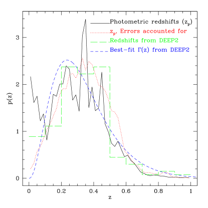
While we have determined the photometric redshift error distributions, we are still far from an understanding of how they affect the lensing signal. There are two effects that must be included:
-
•
The conditional bias, , must be included in our computation of . Because for low , the corrected redshift is larger than , raising (lowering ) once we make this correction. This effect is particularly important at low values of , because is varying more rapidly with source redshift at low redshift. (However, since is lower at low source redshifts, these sources get less weight, so the error they cause is not as high as one might naively expect.) At high redshift, , so the correction will lower the redshift and (raise ), but because varies so slowly with redshift in that regime, we expect that this will only be a minor correction. The majority of the photometric redshifts used are around 0.35-0.4, where the conditional bias goes to zero, so we may expect that its effects will not be too large.
-
•
The conditional scatter must also be included. At photometric redshift more than above the lens redshift (i.e., for most sources in this work, due to our requirement that ), because is an increasing function of source redshift with negative second derivative in this regime, the inclusion of the width of the error distribution will lower the estimate of (raise ). This effect is counter to the effect of the conditional bias at low , and in the same direction as it at high . However, at low , close to , the effect of the -function in the second derivative at is that is actually higher than it would have been without the scatter, i.e. this effect goes in the same direction as the bias at very low photometric redshift.
Figure 9 shows a plot of for lenses at several redshifts, as a function of source redshift, for several different possibilities: straight acceptance of source photometric redshift, use of the photometric redshift corrected for the conditional bias, and corrected for the full photometric redshift error distributions (actual, and best-fit). The fit for the distribution was done by assuming it is a Gaussian with a fixed width but with a mean that is a linear function of . This form was assumed because it is a simple parametrization that can still account for the fact that the error distribution changes sign as we go from low to high . The effects of the mean correction (which raises for and lowers it for ) and the width of the error distribution can clearly be seen in this plot.
Vertical lines show our cutoff of ; fortunately, as shown, this limitation on the photometric redshifts means that even just using photometric redshifts directly, without accounting for the errors, is less likely to cause errors. Furthermore, as shown, the errors in for are downweighted in importance due to our weighting scheme, with weights . Consequently, we can expect to see some cancellation, whereby the large increase in (decrease in signal) for small , which has small weight due to the weighting scheme, is cancelled by the modest decrease in (increase in signal) for large and , which get considerable weight. The extent of the cancellation will be shown in §6.3.
The difference in results between the best-fit Gaussian error distribution versus the actual error distribution is quite small, except for the range that is not used in this work; probably, the best-fit distribution gives higher values of in this range because the fit distribution underestimates the tails that are present in the actual distribution, and the tails help to lower with the actual error distribution for . This result implies that when restricting to the range as in this work, it is unimportant whether or not the method of parametrizing the photometric redshift error distribution is able to account for the tails, as long as the basic shape (mean and width) is correct. However, for analyses that include lower values of , a more careful treatment of the error distribution is necessary.
It is clear from these results that for different limits on source photometric redshift (e.g., without requiring ), the results of photometric redshift errors will vary, and must be re-evaluated if we choose to relax this restriction.
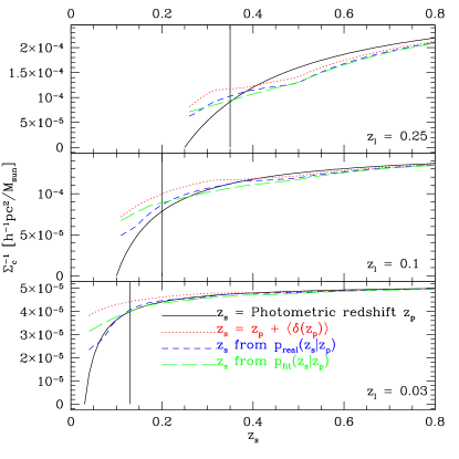
As illustrated by this discussion, the effect of photometric redshift errors is complicated, with several possible effects that will tend to push the lensing signal in opposite directions, and it is difficult to anticipate which effects will turn out to be more important than others for any given lens and source sample. Consequently, we must turn to the systematics test described in §5 to determine the effects of photometric redshift errors on .
We also must consider the effects of errors in the photometric redshift error distribution. Statistical (Poisson) error can be determined via a bootstrap resampling of the DEEP2 matches. The effects of LSS and systematic error are more complex, because correlations between photometric redshift errors are more difficult to model than the correlations between the redshifts used to derive . There are several concerns: statistical errors on photometry; systematic errors on colors; and deviations of galaxy SEDs from templates. For example, if the colors of galaxies depend on environments, we may expect different photometric redshift error distributions for field galaxies versus those in groups or clusters.
6.2 Error comparison
Because we used three methods to compute error estimates on the signal (the analytic expression for the error, the random catalog errors, and the bootstrap errors), we compare the results of the three methods to ensure that they gave comparable results. In general, the results of the three methods were quite comparable, with the exception of two situations. First, for the lower luminosity bins, the bootstrap and random catalog errors were larger than those computed analytically by 15–20 per cent. Second, for the higher luminosity bins, the radial bins that required a sizable boost had larger errors computed using the bootstrap than via the other methods. Because there is some uncertainty on the boost factors (which was also computed using the bootstrap), the uncertainty on the product is approximately when computed using the bootstrap, raising the fractional error by roughly 5 per cent at small pair separations. The larger errors from the bootstrap are more likely to be correct since they take into account errors on the boost factor itself, so these are the errors that were used for the computation of ratios .
The analytic errors are essentially noiseless since they are computed over millions of lens-source pairs. The random catalog errors had the most noise, since they were computed with only 24 random catalogs due to the computational expense involved. If the error amplitude is fit to a power-law , and the noise amplitude is defined as the fractional difference between the actual errors and the best-fit value, then the random catalog errors typically had a noise amplitude of 15 per cent. The bootstrap errors have little to no noise, with a maximum noise amplitude of 5 per cent even for L1 and L6 (which had the fewest lenses) and 1 per cent or lower for the others.
We also checked the covariance between the signal in different radial bins using the bootstrap for all luminosity bins and source samples. We can anticipate that these correlations may become important on angular scales for which the lens-source separation is comparable to the lens-lens separation, since on those scales a given source will contribute to the calculation for more than one lens. We find a typical lens-lens separation to be 7’, which corresponds to comoving transverse separation of 200 kpc in L1, and as high as 1100 kpc in L6. Using the bootstrap resampling for 2500 datasets, we find that for L1, there are correlations as high as 0.2–0.3 starting at radii of 800 kpc between nearby radial bins (generally the 3 nearest radial bins in either direction) but little covariance between the bins for lower radii. The bootstrap procedure naturally introduces noise with standard deviation ( is the number of bootstrap regions) in the correlation coefficients when they are (the noise is less for higher correlations), so the statement that there is little covariance means that the correlation coefficients were consistent with being drawn from a Gaussian distribution . For L6, no covariance is observed within the noise, even for the outermost bins that should be most correlated, since these correspond to a smaller angular scale than for the fainter (more nearby) lenses. Note that our procedure described in §5 automatically takes any covariance between the radial bins into account because it uses the bootstrap.
We also found that our measure of the signal in a given bootstrap-resampled dataset, as defined in §5, has a significant covariance between luminosity bins. This result is unsurprising considering that many of the same sources contribute to the result in different luminosity bins, though the weighting may differ significantly. We found correlations between the results in different luminosity bins as high as 0.30 for adjacent luminosity bins, 0.10 for luminosity bins that were separated by one (e.g. L4 and L6), and consistent with zero for further separations. This kind of correlation must be taken into account (as it is with the bootstrap) for any analysis that utilizes the results in several luminosity bins simultaneously.
As an additional test, we also examined the distribution of values of for each luminosity bin and source sample, computed from the 2500 bootstrap-resampled datasets. This distribution was found to be Gaussian to high accuracy. The Gaussianity is quantified via calculation of the skewness
and kurtosis excess
both of which should be zero for a Gaussian distribution within the noise. For bootstrap subregions, and resampled datasets, the expected variance of the skewness is ( and in our case) and of the kurtosis is (Cramer, 1946). The values of and calculated for a number of different sources samples and luminosity bins were consistent with being drawn from random distributions with mean zero and approximately those variances, and therefore consistent with Gaussianity.
6.3 General systematic tests
In this section, we present results of tests for systematics described in §4.
6.3.1 Random points test
As mentioned in §4.1, we found a nonzero signal computed around random points in the survey region, indicating the presence of a systematic shear in the source catalog that must be accounted for. The shape and amplitude of this signal varies with luminosity bin and source sample, because it is related to angular scale (and therefore different transverse separations for lens samples at different redshifts) and likely varies with source as well.
In principle, if the systematic shear is uniform across the survey, then it will only be revealed on large scales. If the distribution of sources around lenses is circularly symmetric, then the contribution of the systematic shear to the signal averages out, so only edge effects on large scales will show the presence of systematic shear. The effect of this spurious ellipticity is most noticable for the narrow southern stripes, of approximate width 2.5 degrees; our decision not to use them for the work in this paper reduced the observed random catalog signal by approximately a factor of four. However, it is unlikely that the systematic shear is perfectly uniform, and if it fluctuates on small scales then we may also see a random catalog signal at small transverse separations.
As an illustration, figure 10 shows the mean random catalog signal for all 6 luminosity bins, computed with sources.
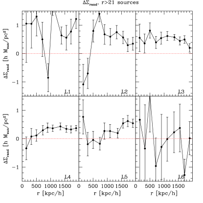
As shown in this figure, there is a clear signal from the random catalogs at large radius; the statistical error due to this signal can be taken into account by the bootstrap. For the brighter sources, , the random catalog signal has slightly different shape, and is shown in figure 11.
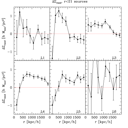
As shown there, the signal is zero at low transverse separation, then becomes positive in the fainter bins, decreasing to zero at larger radii. While this occurs at different radii for L1–L3, the corresponding angular scale is same: roughly 25’. This number is of significance in the SDSS as the separation between adjacent camcols; however, the reason it is showing up here is not entirely clear. For the characteristic redshift of L4, 25’ corresponds to 2.2 Mpc, which is why the signal does not go to zero in that bin; however, it is clearly declining by the maximum radius of 2 Mpc.
If the systematic shear is constant across the survey, then one way to eliminate or at least reduce it would be to only keep lenses that have a reasonably circular distribution of sources around them, since the systematic shear along the scan direction will then cancel out of the calculation of . We implemented this cut, requiring the ellipticity of the distribution of sources around the lens to be less than 0.2, but found that this cut did not significantly decrease the random catalog signal; consequently, we conclude that the systematic shear fluctuates on a scale smaller than the typical distribution of sources around a lens, and did not use this cut for the work in this paper.
6.3.2 45-degree test
In this subsection we describe results of the 45-degree test described in §4.2. This test was performed using the bootstrap with 2500 subsamples. In order to check for a systematic dependent on transverse separation, we did the test in 3 radial bins: 30–100 kpc, 100–600 kpc, and 600–2000 kpc, as well as for the full range 30–2000 kpc. The test was done for each lens luminosity sample separately, and the results were also checked for the combined result averaged over lens luminosity.
Note that the 45-degree random catalog signal was nonzero for all lens-source subsamples, and therefore had to be subtracted just like for the non-rotated signal. Unlike for the real signal, rather than averaging , we average since we do not expect this quantity to vary widely over the radial range used. We checked the error distribution for with the bootstrap and, since it was found to be Gaussian, use a simple test to determine the statistical significance of the 45-degree signal. Since the test involves using just a single variable ( averaged over a given radial range), we use the distribution with a single degree of freedom to calculate -values, the probability for to exceed the given value by chance assuming that it really is consistent with zero. Problems that cause a pure calibration bias alone have no effect on -values since they change both the amplitude of the signal and the errors.
Results for the 45-degree test for all source samples and radial ranges are shown in table 12 averaged over luminosity bins. As shown there, we have no evidence for a 45-degree signal, which indicates that we are not dominated by systematics, since most contribute to the 45-degree signal on the same level as the non-rotated signal. Results for each luminosity bin are not shown, in order to simplify the presentation of results, but we also have no evidence of 45-degree signal in individual luminosity bins. Fig. 12 shows the 45-degree signal averaged over luminosity for each source sample.
| Radial range (kpc) | -value | ||
|---|---|---|---|
| sources, without LRGs | |||
| 1.70 | 2.45 | 0.49 | |
| -0.03 | 0.45 | 0.96 | |
| 0.38 | 0.24 | 0.12 | |
| 0.33 | 0.22 | 0.13 | |
| sources | |||
| -1.72 | 3.04 | 0.57 | |
| -1.17 | 0.55 | 0.04 | |
| -0.13 | 0.25 | 0.62 | |
| -0.25 | 0.23 | 0.26 | |
| LRGs | |||
| 6.37 | 5.31 | 0.23 | |
| -0.17 | 0.91 | 0.85 | |
| -0.21 | 0.45 | 0.64 | |
| -0.19 | 0.42 | 0.66 | |
| All | |||
| 1.44 | 1.90 | 0.45 | |
| -0.47 | 0.34 | 0.17 | |
| 0.09 | 0.18 | 0.63 | |
| 0.02 | 0.17 | 0.88 | |
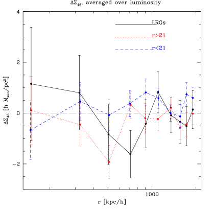
6.3.3 Star-galaxy separation
As described in §4.3, we have good reason to believe that stellar contamination in the source catalog, even at faint magnitudes, is minimal ( per cent for ). However, we tested this hypothesis by computing signal for lenses at low galactic latitude, defined as , and compared the results against the signal at high galactic latitude. In principle, stellar contamination can cause the signal at low galactic latitudes to be lower than the signal at high galactic latitudes. For this test, in order to maximize signal-to-noise, the signal was computed using lenses in L3–L6 combined, since most of the signal comes from those bins. This process was done for both the and sources separately, where we expect most stellar contamination to be in the sample.
The results of the test are shown in table 13. As shown, while the signal in the low galactic latitude sample is lower than that in the high galactic latitude sample, the signals are statistically consistent with each other for and cases. This result, combined with the results from GOODS shown in §4.3, supports our assertion that stellar contamination is negligible in our catalog. For bounds on the error in the signal due to stellar contamination, we use the results from GOODS with the binomial distribution as in §4.3.
| Sources | Sources | 68% CL | 95% CL | |||
| lower | upper | lower | upper | |||
| Stellar contamination test, §6.3.3 | ||||||
| without LRGs, | without LRGs, | 0.86 | 0.78 | 0.94 | 0.70 | 1.03 |
| , | , | 0.92 | 0.84 | 1.01 | 0.76 | 1.11 |
| Seeing comparison, §6.3.4 | ||||||
| without LRGs, bad seeing | without LRGs, good seeing | 0.99 | 0.92 | 1.08 | 0.85 | 1.17 |
| , bad seeing | , good seeing | 1.00 | 0.92 | 1.09 | 0.84 | 1.19 |
| comparison, §6.3.5 | ||||||
| without LRGs, , -band | without LRGs, , -band | 1.11 | 1.02 | 1.20 | 0.94 | 1.30 |
| without LRGs, , -band | without LRGs, , -band | 1.12 | 1.04 | 1.21 | 0.96 | 1.30 |
| , , -band | , , -band | 0.89 | 0.80 | 0.99 | 0.71 | 1.10 |
| , , -band | , , -band | 1.24 | 1.13 | 1.37 | 1.03 | 1.50 |
| versus band comparison, §6.3.6 | ||||||
| without LRGs, -band | without LRGs, -band | 1.06 | 1.00 | 1.12 | 0.95 | 1.18 |
| , -band | , -band | 1.04 | 1.00 | 1.07 | 0.97 | 1.11 |
6.3.4 Seeing dependence of calibration
As described in §4.4, we also used the systematics test to compare the signal computed with sources that had PSF sizes greater than and less than the median. The results of the test using L3–L6 lenses are shown in table 13. As shown there, the signals are statistically consistent with each other, indicating that we do not have to worry about seeing-dependent calibration of the shear.
6.3.5 dependence of calibration
As described in §4.5, we used the systematics test to compare the signal computed with sources with versus with . This exercise was done in both the and bands separately, and results are shown in table 13. As shown there, there is no evidence at the level for a systematic calibration offset that depends on resolution factor .
This result is important because recent tests have indicated that the source catalog used in H04 did have an -dependent calibration, with the calibration changing by as much as 50 per cent from the lowest to the highest. When averaging over all sources, this effect caused the calibration for that paper to be too low by approximately 15 per cent (only sources were used for that work; since the LRG sample and the sample is, on average, at lower , the offset is even worse for those samples). Tests to determine the source of the problem were not definitive, but seemed to rule out selection biases. The basic conclusions of that paper, namely the 99.9 per cent stat+sys confidence intervals on the intrinsic shear, are essentially unaffected by this problem, since we assumed up to 20 per cent shear calibration bias when computing the confidence intervals. However, this finding highlights the importance of our results here, which is that this catalog does not have a statistically significant -dependent calibration.
6.3.6 Systematic differences between bands
While for most tests we used the shape measurements averaged over both and bands, we also compared the signal computed using only one band versus the signal computed using the other. This test was done separately for and sources. As shown in table 13, there is no sign of a systematic discrepancy between the signal computed using the shape measurements in either band individually, so to improve statistics we will henceforth use the shape measurement averaged over bands.
6.3.7 Boosts
The boost factors generally follow expected trends, decreasing with radius and increasing with luminosity. Furthermore, they are largest with the sources, which have the largest overlap in redshift range with the lens sample; less with the sources; and the smallest with the LRG sample, since those are chosen specifically to avoid contamination from low-redshift () galaxies.
A systematic effect at the smallest radii ( kpc) is revealed by the boost factors. While they should, in principle, be monotonically decreasing, we found that for the brightest lens samples, they actually increase from 20–30 kpc, then follow the expected trend of decreasing for kpc. In H04, this trend appeared for even larger radii; however, for that work, our source catalog did not include deblended children, so this result is expected. This source catalog does include deblended children, so we do not expect a loss in lens-source pairs for small transverse separation due to the loss of deblended children. However, very bright galaxies, for which this effect is noticable, are large enough that at those separations, their light could make it impossible to detect much smaller, faint galaxies. This could explain the fact that this effect is more noticable for the fainter sources than it is for the sources. In order to avoid strange selection effects due to this problem, this work only uses kpc for the analysis.
Plots of the boost factor are shown in Fig. 13. The top plot shows the trends of the boost with luminosity bin for the sources; the bottom shows the variation of boost with source sample for L5 lenses. The problem with at kpc is clearly visible in this plot, especially for L6.
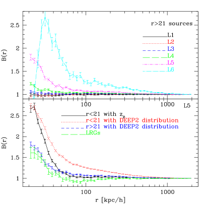
A close examination of the boost factors reveals a systematic effect at small transverse separations that affects any analysis of galaxy-galaxy weak lensing done using SDSS data. From plots of the boost factor at small transverse separation computed using LRGs as sources, it became apparent that there is a deficit in lens-source pairs below a certain radius. This deficit manifests itself in the boost factor actually dipping below 1 (i.e., ), which is not physical. This deficit also is present for the and samples, though it is harder to notice because of the fact that there are physically-associated pairs at the affected radii. We determined that this effect is due to either an instrumental effect or something in the Photo pipeline (rather than due to some selection effect in our catalog, error in signal computation, or actual physics) due to the following factors: (1) it occurs at a particular angular (not physical) scale, most noticably around 50” though it extends up to about 90”, (2) the effect is noticable with two different catalogs, the one from this work and from H04, which were processed with completely independent software pipelines from the Photo outputs, (3) it is most noticable for lenses that are bright in apparent magnitude, (4) it is most noticable for low surface-brightness sources, and (5) we see the effect even if we compute the signal around bright stars instead of around galaxies. While a hint of this effect can be seen for from LRGs in Fig. 13, it is more obvious in Fig. 14, which shows a plot of the correlation function between bright () stars and high-redshift LRGs, where there is a non-zero correlation function at small separations because of low-redshift quasar contamination in the star sample. This plot was computed using only low surface-brightness sources (those with a value below the median), and is shown as a function of star magnitude.
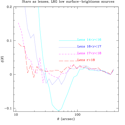
The effect turns out to be due to a problem in determination of the sky level around bright objects (stars or galaxies). The sky level is determined in overlapping boxes of size 256 pixels (approximately 100”) and linearly interpolated on the 128 pixel (50” scale), using a clipped median666For more information about the sky level determination, see http://www.sdss.org/dr3/algorithms/sky.html.. We expect the sky level near bright lenses (within about 1’) to be higher than the global sky because light from the lens galaxies extends out to a large angular separation, and we do not want that extra light to be included in the flux from the sources in that region. So, we do want the sky level to be influenced by the presence of the bright objects. However, our results suggest that the sky level determination is overly influenced by the presence of bright objects, with the sky level being set too high near them. The problem is different for each band. This change in the sky level has several effects: (1) some sources are not detected at all by the Photo software, (2) some are detected, but due to the faulty sky level, the magnitudes, colors, and shape measurements determined by model fits to the light profile are off, and therefore they are not included in our source catalog because of magnitude or cuts or OBJC_TYPE failure, or are included but with these quantities computed wrong, and (3) our computed redshift distribution of these sources is likely wrong because of the incorrect fluxes. Furthermore, because this effect can vary from band to band, the colors are incorrect as well, affecting both photometric redshift determination and selection of the high-redshift LRG sample.
To test that this effect is indeed the cause of the observed effect, we used the Photo reductions to compute the averaged sky level as a function of angular separation from bright galaxies (we except the effect to differ around stars versus galaxies, because galaxies are extended and therefore affect more pixels). This computation was done in each band, and we verified that the sky flux level around bright galaxies is indeed higher than the baseline value computed around faint galaxies, by a quantity we call in each band. For such small angular separations, we expect that should be higher than that baseline, so much of the rise at small angular separations is not spurious. Fig. 15 shows a plot of the average sky flux in the band as a function of angular separation from lens galaxies with apparent magnitudes as labeled on the plot. We can make a naive calculation of the effect of this problem (assuming that all of is spurious and that the only effect was to change the surface brightness of the faint source without changing its size) at 40” for a circular source galaxy 4” in diameter at magnitude 21.5. The flux for such an object is 2.5 nanomaggies, and since its area is 12.5 square arcsec, then if the lens is at , with nanomaggies per square arcsecond, its true flux should have been 5.0 nanomaggies, a full factor of two higher, giving it a true magnitude of 20.8, a highly significant offset from the observed value. For lenses around , a large fraction of the sample, is smaller, but we still expect a “true” magnitude of 21.0. Of course, this is just a crude estimate, and a more careful calculation of what happens to the fits to the light profiles when the sky level is changed is necessary. This calculation is actually quite complicated because the change in sky flux changes the effective radius of the source from the fits, so not only is the flux underestimated within the area of the galaxy, light is also lost due to the underestimated size. However, when we tried applying this naive correction, we found that we overcompensated for this effect, so it seems clear that some of is not spurious (as would be expected for such large, bright lenses, for which some of the light does indeed extend to these radii).
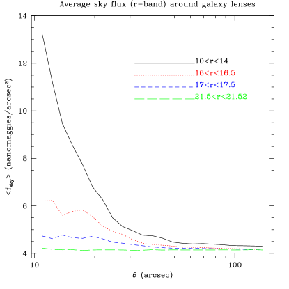
There are several implications of this effect for our work. First, while figure 14 shows what looks like a dip in the boost factor below 90” and most prominently at 50”, with it then rising at lower separations, our findings suggest that the boost factor is actually underestimated for all radii below the 50” level, though it is impossible to actually see this effect due to the physically-associated pairs. (Note, however, that if the problem is due to the lens galaxies light profile falling off faster than the linear interpolation scale of the sky level, then the effect should be worst around the 50” scale and, if anything, somewhat better at smaller separations.) It seems that we have lost pairs either because the sources were not identified by Photo at all, because their fluxes and sizes were miscalculated so they failed our magnitude, , or OBJC_TYPE cuts, or (for the high-redshift LRG sample) because their colors were wrong. Furthermore, for the pairs that were included, we must be concerned about incorrect shape measurement and redshift distributions. In general, this error will tend to lower the measured signal, since the underestimated boosts lower the signal, and the effect of underestimating the flux is, on average, to make us think the galaxies are fainter and more distant, overestimating and underestimating . Since at 50” we see a 5 per cent effect, and it may be worse at smaller , though likely not much worse since the problem is due to the interpolation, we place a bound on the error due to this effect of , but we emphasize that more study is necessary to quantify this effect more precisely.
We attempted to correct for this effect by excluding regions near objects (stars or galaxies) with saturated pixels, or about 1.5 per cent of the sample, and regions within 60” of galaxies, or about 8 per cent of the sample.777We thank Ryan Scranton for providing the necessary masks and mask utilities to allow us to perform this test. However, with these restrictions, we still see the effect at approximately the same level as before. This fact indicates that most of the problem is due to the galaxies that comprise the majority of our lens sample rather than due solely to the very brightest subsample of lenses.
In future work, we will attempt a more detailed modeling of this problem. For most of our results, we do not attempt to correct the boost factors, which are clearly underestimated, though we will show what happens to the results if we try a naive correction; since only small separations are involved, the change in the signal averaged over radius due to this effect is small. Furthermore, while we have estimated rather large values for the magnification bias at small separations for the and LRG samples, this sky level problem makes it effectively impossible to make any detection of magnification bias with the SDSS using MAIN spectroscopic sample lenses and working at angular separations of less than approximately 90”.
The final test performed in this section was to compare the signal computed for the bright and faint halves of the brightest bin (L6) separately and then averaging them (i.e., taking the average value of ) versus the signal computed by averaging over the whole luminosity bin, as we usually do, to get the average values of and . The concern is that due to the non-uniformity of the boost factor, with both the boost factor and signal rapidly increasing in this bin, our averaging process may bias the signal. Our tests indicate that for the both and sources, the effect of this averaging is less than a 1 per cent effect even for L6; consequently, it must be negligible for the other bins, for which the signal and boosts are varying less rapidly.
6.3.8 Intrinsic Alignments
When computing the expected contamination due to intrinsic alignments, we must do the computation separately for each luminosity bin and source sample because the contributions may vary with lens mass (and therefore luminosity) and with source sample (more distant source samples will have fewer physically associated lens-source pairs). Furthermore, the procedure should be done as a function of radius, since limits on the intrinsic shear vary with radius. We split the data into 3 radial ranges with limits and . This estimate assumes that the boost factors are entirely due to physically associated pairs, and ignores the magnification bias estimates in table 6.
The signal contamination due to intrinsic alignments can be computed as follows. First, we determine the fraction of lens-source pairs that are physically associated. For each lens sample , source sample , and radial bin , we compute
| (46) |
where is the area of the annular bin centered at , and the value of is determined via the bootstrap.
Then, for a given radial range, we can compute the estimated contribution of intrinsic alignments to the lensing signal via
| (47) |
In order to avoid excessively low (or even non-physical negative) values of , we had to correct for the sky level effect that suppresses at small radii. This correction was done as follows. For the LRG sample, for which this effect is most noticable, we examined for all lens samples. We found the minimum value at , and assumed that the effect was actually the same at all (and could not be observed because for those radii). So, for , we multiplied the signal and by ; for , we multiplied the signal and by if , and by otherwise. This correction is very rough, since it assumes that the sky level effect is the same for all source samples, and that the sky level effect only changes the boosts without having an effect on the shear or redshift calibration. However, our estimate of contamination from intrinsic alignments in table 14 is still conservative, because we ignore the fact that magnification bias contributes to the boost factors at small radii. For the purpose of this calculation, the 99.9 per cent stat+sys confidence intervals from H04 have been reduced by a factor of 0.6 so they will be rather than bounds.
| Lenses | , | , dist | LRG | |||||||
|---|---|---|---|---|---|---|---|---|---|---|
| kpc | ||||||||||
| L1 | ||||||||||
| L1 | ||||||||||
| L1 | ||||||||||
| L1 | ||||||||||
| L2 | ||||||||||
| L2 | ||||||||||
| L2 | ||||||||||
| L2 | ||||||||||
| L3 | ||||||||||
| L3 | ||||||||||
| L3 | ||||||||||
| L3 | ||||||||||
| L4 | ||||||||||
| L4 | ||||||||||
| L4 | ||||||||||
| L4 | ||||||||||
| L5 | ||||||||||
| L5 | ||||||||||
| L5 | ||||||||||
| L5 | ||||||||||
| L6 | ||||||||||
| L6 | ||||||||||
| L6 | ||||||||||
| L6 | ||||||||||
For this calculation, we assumed that for the and LRG samples is the same as that for the sample. While this assumption is not fully justifiable, and means that the actual estimates of the contamination should not be taken too seriously, the size of the confidence intervals are likely still trustworthy.
Here we discuss the results in table 14. The entries with as bounds are those for which H04 could not place any constraint on . As shown, because of the poor constraints at low luminosities (due to the fact that the contamination fractions are so low that there were very few lens-source pairs with which to study the intrinsic alignments), no strong constraints on the contamination of signal due to intrinsic alignments could be placed in H04. However, the fact that the average signal for these ranges is entirely reasonable suggests that the contamination by intrinsically associated pairs is not causing a large problem. For , use of rather than photometric redshifts leads to very large contamination fractions and therefore very loose constraints on . The fact that the contraints on intrinsic alignments for , , and LRG samples are quite different, generally tightest on LRGs and loosest on , yet the results agree quite well (as will be shown in §6.4.4) suggests once again that we do not have a major problem with contamination by intrinsic alignments. For small radii, the (with ) and samples, we assign uncertainties due to intrinsic alignments of per cent for L3–L5 and per cent for L6; for LRGs, per cent for L3–L5 and per cent for L6. For large radii, the (with ) sample, we assign uncertainties of per cent for L3–L5 and per cent for L6; for , per cent for L3–L5 and per cent for L6; and negligible for LRGs. These constraints were assigned by comparing the constraints on to the characteristic in the table.
6.3.9 Corrections for non-volume limited sample
As described in §4.9, we must consider the effects of differences in the mean weighted luminosity of the subsample when computed with different source samples or redshift distributions for the same sample. Using a simple model for , we can compute the expected change in the signal from Eq. 33, and expected ratios
| (48) |
We have no need for these corrections for L1 and L2, since for those samples all source samples are essentially at infinite redshift, and is exceedingly small. Using our results for L3–L6, we find , 0.43, 0.48, and 0.33 respectively.
We must consider several types of corrections. First, we consider signal comparisons for sources, with different methods of determining . The maximum variation in luminosity found when comparing among the methods is 0.0023, 0.0028, 0.0046, and 0.0027 for L3–L6 respectively, which gives expected ratios of 1.0004, 1.0012, 1.0022, 1.0008, far too small to be detected considering our statistical errorbars; consequently, we do not apply any correction when comparing between the various methods of computing for the sample. Next, we consider comparisons within the source sample, different methods of comparing . The maximum variation in luminosity is 0.0017, 0.0033, 0.0041, and 0.0017, again giving expected ratios similar to those for , far too small to measure. For comparisons within the LRG sample, there was no detectable difference in the weighted luminosity since the source redshift distributions varied very little and are all essentially at infinity.
The final test is the comparison of the luminosities between the different source samples (, , and LRGs) to ensure that the ratio test should not have some correction due to their different weighted luminosities. In general, the weighted luminosity of the sample was lowest, and the LRG sample was highest. We find maximum of 0.0092, 0.016, 0.016, and 0.006 (comparing LRG to ), giving expected ratios of 1.002, 1.007, 1.006, 1.002. Given that these ratios represent a difference in overall calibration of less than 1 per cent, much lower than our bounds on the calibration, we find that we need not apply any correction for the change in mean weighted luminosity when comparing the signal from different source samples.
6.4 Redshift systematic tests
In this section, we describe our application of the systematics test to assess which methods of redshift distribution determination are optimal. First, for each group of sources ( without LRGs, , and LRGs), we compared the various methods of determining the redshift distribution. Next, we compared the signal determined using each of these three samples, to make sure that our results are consistent. In each case, this test was done individually for each luminosity bin, because we can expect that different lens redshift samples will sample different parts of the source redshift distribution, and therefore results may differ systematically across the luminosity bins. However, we also use the results averaged over luminosity bins for greater statistical power. Plots of the signal will be shown in §6.4.4.
All errorbars shown in this section are statistical errorbars from the computation of signal only; they do not include systematic error on the shear or redshift distributions, or statistical error in the determination of redshift distributions or photometric redshift error distributions.
6.4.1 Bright () sources
For the sources, several methods of redshift distribution determination are compared:
-
1.
The redshift distribution from COMBO-17,
-
2.
The average redshift distribution from DEEP2,
-
3.
Photometric redshifts from kphotoz directly,
-
4.
Photometric redshifts, corrected for the conditional bias only,
-
5.
Photometric redshifts, corrected for the best-fit error distribution, and
-
6.
Photometric redshifts, corrected for the actual (noisy) error distribution.
The first two methods involve averaging over a redshift distribution to determine without the use of photometric redshift information to eliminate physically associated pairs. The final four methods use photometric redshifts to select sources with to eliminate physically associated source-source pairs. The two methods involving distributions use all galaxies, including those for which photometric redshifts were not available and those passing the high-redshift LRG cuts; the last four methods only involve non-LRGs, since the photometric redshift error distributions for non-LRGs and LRGs are quite different.
In this section, we compare the results using 30–2000 kpc, without subdividing this region, since changes in the redshift distribution only affect the amplitude of the signal, and not its slope. Furthermore, we only use luminosity bins L3–L6 since the majority of the signal is in those bins; adding L1 and L2 actually lowers the slightly. Since changes in redshift distribution will tend to have a greater effect on the higher-redshift lenses, we are also interested in the results as a function of luminosity bin. Table 15 shows the results for the ratios for the selected ranges of radii, including 95 per cent confidence intervals computed via the non-Gaussian error computation for correlated variables (correlations between the signal computed using method 1 or 2 and methods 3–6 were of order 0.75, and correlations among methods 3–6 were of order 0.98). Because of the high correlations, the ratios were determined to high accuracy. Results are shown for L3, L6 (so that comparison can illustrate trends in lens luminosity), and the average signal in bins L3–L6.
| Sources | Sources | |||
|---|---|---|---|---|
| L3 | L6 | L3–L6 | ||
| DEEP2 | ||||
| DEEP2 | , fit | |||
| DEEP2 | , bias | |||
| DEEP2 | , | |||
| DEEP2 | COMBO17 | |||
| , fit | ||||
| , bias | ||||
| , | ||||
| COMBO17 | ||||
| , fit | , bias | |||
| , fit | , | |||
| , fit | COMBO17 | |||
| , bias | , | |||
| , bias | COMBO17 | |||
| , | COMBO17 | |||
We can see from table 15 that at 95 per cent confidence level (CL), the results from these different ways of computing all give results that have overall calibration within 15 per cent of each other. First, we compare the two redshift distributions shown in the table; this comparison is on line 5 of the table. As shown, the distributions from COMBO-17 and DEEP2 give results that have no difference in overall calibration, and this calibration can only differ by to per cent at the 95 per cent CL when averaged over luminosity bins. Since Fig. 7 shows how similar these distributions are for , this result is not too surprising.
Next, we compare the results for the different ways of using photometric redshifts. First, we can consider the difference between using photometric redshifts directly and correcting for their mean bias (but not the width of the error distribution), shown in line 7. As demonstrated by the results for L3–L6, correcting for the mean bias lowers the signal by about 3 per cent, and the results are statistically inconsistent with the results without any correction for photometric redshift error at the 95 per cent CL. We expected the correction for the mean bias to lower the signal because for low photometric redshift, so correcting for the mean bias will raise the assumed source redshift and , lowering (while for high photometric redshift, so correcting for it should raise the signal, the effect at low photometric redshift is apparently more important since varies more strongly with at low despite the weights proportional to that make higher redshift sources more important). We next consider what happens when we go from including the mean bias only, to including the full error distribution (line 13). As shown, including the width of the error distribution then raises the signal by 5 per cent; the results corrected for only the mean bias versus using the full error distribution (bias and scatter) are statistically inconsistent at approximately the level, which means that including the width of the error distribution is very important. This increase in signal when we include the scatter is consistent with our expectation that scatter will lead to decreased , at least for the values used here (at lower it may actually raise ). The next comparison is using photometric redshifts directly versus including the full error distribution, line 8; consistent with combining the aforementioned results from lines 7 and 13, we find that including the full error distribution increases the signal compared to no correction at all by approximately 2 per cent, though the results are marginally consistent at the level. This near agreement is due to the effects from the mean bias and width of the distributions cancelling out; the nearly exact cancellation was impossible to predict in advance, which is why this systematics test is so useful.
We can also use these results to place approximate bounds on the calibration uncertainty due to statistical error in the photometric redshift error distribution. We place these bounds using the comparison between no correction at all, correction for , and correction for the full error distribution, which gives approximately per cent calibration uncertainty (95 per cent confidence level). This result is comparable to the Poisson errorbars (determined via bootstrap resampling of the photometric redshift error distribution) which are per cent for lens redshift , lower for lower lens redshift; we use the per cent figure to include extra uncertainty due to the effects of LSS.
Another informative test is the comparison between the results using the best-fit error distribution versus the actual error distribution. When plotted against each other, the best-fit distribution did show some significant differences from the actual one; for example, it did not account for the tails in the distribution very well. This comparison is on line 11 of table 15; as shown, use of the best-fit error distribution rather than the actual one increases the signal by about 3 per cent, and the two results are inconsistent at the level. The sign of the discrepancy is in accordance with the results for in Fig. 9. While the magnitude of this bias is clearly not large, since the difference is statistically significant, it seems that it would be preferable to use the actual error distribution to avoid this bias altogether.
Finally, we compare the results using redshift distributions versus using photometric redshift error distributions, lines 4 (DEEP2) and 15 (COMBO-17). We find that the signal is 3 per cent lower when we use either redshift distribution than when we use the photometric redshift error distributions; however, the two results only differ by about , so the difference in calibration is not statistically significant. However, as mentioned previously and demonstrated in Fig. 13, there is significantly more contamination from physically associated pairs when we use a distribution for rather than using photometric redshift information to remove that contamination. Since there is no clear discrepancy due to the use of the redshift distributions versus photometric redshifts with error distributions, but the use of redshift distributions can lead to higher systematic error due to intrinsic alignments, we will henceforth use photometric redshifts with the actual error distributions for the sample when comparing against the signal from other source subsamples.
Another systematics comparison that was completed was the computation of signal with versus with without correcting for photometric redshift errors. If our understanding of photometric redshift errors is correct, then we expect the signal at high to be lower than the signal at low by a statistically significant amount. Indeed, the ratio ; the confidence interval is , so the discrepancy between the two samples is and has the correct sign. When we correct for photometric redshift error, the discrepancy still exists at the level; it is 0.86, with confidence interval . The fact that correcting for photometric redshift errors helps reduce the discrepancy indicates that we are understanding these errors properly. The fact that there is still a discrepancy at the level is not too alarming, because as mentioned previously, the errors used here are purely statistical. Once we add the overall calibration uncertainty, the discrepancy between the two samples is only and therefore not of concern.
6.4.2 Faint () sources
For the sample, two methods of redshift distribution determination were considered:
-
1.
The redshift distributions from COMBO-17, , and
-
2.
The average redshift distribution from DEEP2 for .
In both cases, distributions were used, so we had no way of eliminating physically-associated lens-source pairs; however, since the sample is, on average, at higher redshift than the lenses, this procedure is less important than for the sample. In both cases, high-redshift LRGs are included in the sample. As in the previous subsection, we consider results from 30–2000 kpc. Results for are shown in table 16; since only one comparison is being made, we show results for all luminosity bins.
| Lens luminosity | with 95 per cent CL bounds |
|---|---|
| L3 | |
| L4 | |
| L5 | |
| L6 | |
| L3–L6 |
Not surprisingly, the minor discrepancy () that exists for L3–L4 becomes worse for the higher redshift lenses, since they are closer to the peak of the distribution and are therefore more sensitive to details of the distribution. For L5, the discrepancy is and for L6, , with the result averaged over luminosities a 5 per cent discrepancy, and the two signals being different at the level. Consequently, while the difference in signals is relatively small, we are able to use the systematics test to determine it to very high accuracy. The fact that the distribution from DEEP2 gives slightly higher results implies that it gives on average slightly lower and therefore is at lower redshift on average. This result is not entirely surprising, since the DEEP2 distribution is specific to our lensing catalog, but the COMBO-17 distribution was for photometric galaxies in general, and our lensing cuts will tend to eliminate higher-redshift galaxies more than lower redshift ones. This understanding is in accordance with Fig. 7, which shows both distributions for . Consequently, for the remainder of this paper, the DEEP2 redshift distribution will be used for the sample.
6.4.3 LRG sources
For LRGs, the signal was computed two ways:
-
1.
Using photometric redshifts directly, for , and
-
2.
Using redshift distributions determined via the inversion procedure from Padmanabhan et al. (2004) for .
Besides these two methods of comparing the redshift distribution, we did several tests to ensure that our cuts on the LRG sample were optimal. Using method 1 to determine redshifts, we recompute the signal twice, once with the requirement that and then with ; these stricter cuts should help eliminate more of the low-redshift contamination (this contamination is a concern because we would be vastly overestimating its redshift and , and underestimating ). If the signal computed using these cuts is similar to that computed with our cut, , then we can be assured that the role of low-redshift contamination is minimal. In addition, we also compute the signal using photometric redshifts directly from to ensure consistency with the full sample, in case there is contamination in the . Results for the ratio test are shown in table 17.
| Sources | Sources | |
|---|---|---|
| , | ||
| , | ||
We can come to several conclusions from this table. Lines 1–3 show the results of the systematics tests: using photometric redshifts directly for the full sample with and , versus requiring (line 1), (line 2), or (line 3). As shown, we see no sign of any systematic discrepancy. This result is useful because it suggests that our photometric redshift and color cuts are sufficient to eliminate low-redshift contamination to a negligible level, so there is no need to impose stricter cuts such as those listed above, which also lower the statistical power of this subsample. Line 4 shows a comparison of the results using photometric redshifts directly for versus using the inversion method from Padmanabhan et al. (2004) for . As shown, the results are completely statistically consistent. This result is not surprising, since the LRG sample is at much higher redshift than the lenses, and therefore small changes in the redshift distribution have little effect on the final results. Because of the larger numbers of LRGs in the sample, we will henceforth use the full LRG sample with photometric redshifts directly when comparing against other subsamples. When considering the variation in calibration between the samples in table 17, we conclude that the calibration uncertainty in the LRG signal due to redshift distribution determination is per cent at the level.
6.4.4 All
In this subsection we compare the results from the three source samples (, , and LRGs) to check that they are consistent. As mentioned in the previous sections, we will use the photometric redshifts with the full error distributions from DEEP2 for (without LRGs), the redshift distribution from DEEP2 for the sample, and photometric redshifts directly for the LRG sample.
Furthermore, in contrast to the previous sections, our concern here is not merely overall calibration; since the different source samples have different boost factors and different random catalog signals, it is important to check for radius-dependent effects. In principle, we could also measure the ratios for several radial ranges. However, the for these comparisons was not high enough to give reasonable errorbars. Consequently, we only consider larger ranges of 150–2000 kpc and 30–2000 kpc. The reason for using the 150–2000 kpc range is that even for L6 it excludes the angular separations ” for which the boost factor has the difficult to quantify systematic due to sky subtraction, and it excludes the radii for which magnification bias may be important. Consequently, 150–2000 kpc is a more systematic-free ranges. Results are shown in table 18.
| Lenses | 30–2000 kpc | 150-2000 kpc |
|---|---|---|
| without LRGs versus | ||
| L3 | ||
| L4 | ||
| L5 | ||
| L6 | ||
| L3–L6 | ||
| without LRGs versus LRGs | ||
| L3 | ||
| L4 | ||
| L5 | ||
| L6 | ||
| L3–L6 | ||
| versus LRGs | ||
| L3 | ||
| L4 | ||
| L5 | ||
| L6 | ||
| L3–L6 | ||
We can draw several conclusions from this table. First, the fact that the ratios using 30–2000 and 150–2000 kpc are so similar illustrates that even with our concern about the systematic in the boosts at low values of transverse separation, use of the full radial range does not cause obvious problems. Second, there seems to be some luminosity-dependence of the overall calibration difference between the samples (especially versus ), but the errorbars on individual luminosity bins are large enough that no definite statement about this can be made. Finally, when averaged over all luminosities, the results for the three source subsamples agree well within errorbars. We see no suggestion that there is anything fundamentally wrong with any of these three samples, either in the shear calibration, redshift distributions, or other systematics, and consider the consistency of the samples to be established at the 10% level ().
Here we show plots of the signal. Fig. 16 shows the signal from L5 for the three samples to illustrate our finding from the systematics test that there is no systematic calibration offset between the three samples. Fig. 17 shows the signal averaged over source samples for all 6 luminosity bins, with statistical errorbars only, and the results of halo model fits to the signal as described in Seljak et al. (2005) and Mandelbaum et al. (2004). In order to allow the values shown on the plots to be converted to shear , table 19 includes for each lens and source sample combination.
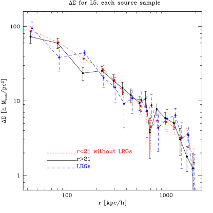
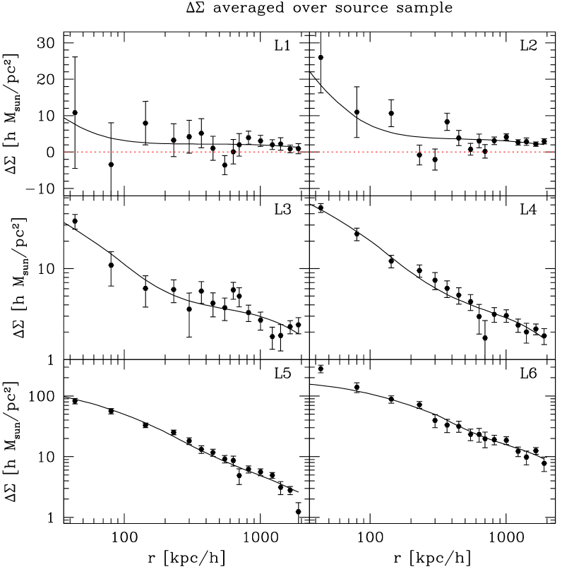
| Lenses | , | ||
| LRG | |||
| L1 | 5.2 | 5.3 | 5.5 |
| L2 | 7.2 | 7.4 | 7.8 |
| L3 | 10.2 | 10.5 | 11.4 |
| L4 | 13.3 | 13.5 | 15.4 |
| L5 | 16.1 | 15.9 | 19.0 |
| L6 | 18.1 | 17.1 | 22.0 |
7 Conclusions
Using the systematics test, we have estimated the effects of redshift distribution errors and other systematics on the lensing signal. As a summary, table 20 lists those systematics that are significant at approximately the 1 per cent level or higher. Systematics are only estimated in this table for the redshift determination methods for each sample that we have selected to use in this and future works (e.g., we do not show results for the use of redshift distributions for the sample). We must emphasize that the estimates of the calibration uncertainty due to these effects is generally only relevant for this work, and their effects for other works must be assessed using the lens/source catalogs used for those works. For those systematics that have some nontrivial dependence on lens sample and/or radial range, rather than listing a value in this table, we refer the reader to the appropriate table/section. We have not included the following systematic effects because they are expected to be at the 0.1 per cent level: atmospheric refraction, camera shear, the density-systematic shear correlation , and non-uniformity of the boost factor.
| Systematic | Lenses | Sources | Radii | bounds |
| Redshift distribution calibration | ||||
| Error in | All | All | ||
| Redshift failures from DEEP2 (table 4) | All | All | , | |
| Statistical error in | All | All | Table 9 | |
| LRG redshift distribution failure | All | LRGs | All | |
| Overall redshift calibration | All | All | ||
| Overall redshift calibration | All | All | ||
| Overall redshift calibration | All | LRGs | All | |
| Other systematic effects | ||||
| Shear calibration bias (§2.2.2) | All | All | ||
| Shear calibration bias | All | All | ||
| Shear calibration bias | All | LRGs | All | |
| Stellar contamination (§6.3.3) | All | All | ||
| Stellar contamination | All | All | ||
| Stellar contamination | All | LRGs | All | |
| Intrinsic alignments (§6.3.8) | L3–L6 | All | Table 14 | |
| Intrinsic alignments | L3–L6 | All | Table 14 | |
| Intrinsic alignments | L3–L6 | LRGs | Small | Table 14 |
| Magnification bias (§4.7.3) | L3–L6 | Small | Table 6 | |
| Magnification bias | L3–L6 | Small | Table 6 | |
| Magnification bias | L3–L6 | LRGs | Small | Table 6 |
| Photo sky level error (§6.3.7) | All | All | Small | |
| Overall uncertainty | L1–L4 | Small | ||
| Overall uncertainty | L1–L4 | Large | ||
| Overall uncertainty | L5–L6 | Small | ||
| Overall uncertainty | L5–L6 | Large | ||
| Overall uncertainty | L1–L4 | Small | ||
| Overall uncertainty | L1–L4 | Large | ||
| Overall uncertainty | L5–L6 | Small | ||
| Overall uncertainty | L5–L6 | Large | ||
| Overall uncertainty | L1–L4 | LRGs | Small | |
| Overall uncertainty | L1–L4 | LRGs | Large | |
| Overall uncertainty | L5–L6 | LRGs | Small | |
| Overall uncertainty | L5–L6 | LRGs | Large | |
The first section of table 20 includes a summary of the findings regarding the redshift distribution calibration, and ends with a calculation of the overall calibration uncertainty for each sample due to redshift distribution-related factors. The second section includes a list of other factors that lead to calibration uncertainty that have been discussed in this paper. The table ends with an estimate of the overall calibration uncertainty at the level for various lens, source combinations and ranges of radii. The estimates are somewhat rough, in the sense that they cannot include all details of the error estimates completed in the text, and consequently a better idea of the magnitudes of some of the errors can be found by reading the appropriate sections of the text.
In this table, we refer to “small” versus “large” radii, where the distinction between the two is that on “large” radii the estimates only include the calibration uncertainties such as stellar contamination, shear calibration, and redshift distributions, but for “small” radii, we must also be concerned about systematics such as intrinsic alignments, sky subtraction effects, and magnification bias. The definition of small versus large radii varies by luminosity bin, and the approximate transition between the two occurs at 40, 60, 80, 100, 140, and 200 kpc for L1–L6 respectively.
The overall uncertainty estimates in table 20 were computed using one of several possible methods. The difficulty is that by definition systematic errors are those with unknown probability distributions, so it is not clear how to combine confidence intervals for multiple effects. The first possible method, the most conservative, would be to linearly add together the upper bounds for all the independent sources of error to get an overall upper bound, and similarly for the lower bound. This method does not require us to make any assumptions about the probability distributions for these systematic errors, most of which are very likely not remotely Gaussian. The second approach would be to assume a uniform distribution of the systematic error between the bounds given in the table. With this assumption, we can find the mean and the standard deviation for each systematic error, average the means and add the standard deviations in quadrature, and use those results to find combined bounds. This approach is also justifiable, since the use of a uniform distribution leads to rather generous confidence intervals, but the results are still smaller than the very conservative bounds from the first approach. The final approach would be to add the lower bounds in quadrature, and add the upper bounds in quadrature. For table 20, we used the bounds from the second method (assuming a uniform distribution); the results using the first method are about 50–100 per cent larger, and using the third method are about 0–10 per cent larger.
In this paper, we have sought to understand the various sources of calibration uncertainty and other systematics in the galaxy-galaxy weak lensing signal computed using our lens and source catalogs. As more data is collected, we will be able to perform these tests to constrain the systematics with greater precision. The understanding we have gained from the systematics test will allow us to use this catalog for many scientific applications (studies of the relation between mass and luminosity, mass and stellar masses, halo profiles as a function of environment, and others) with an understanding of the implication of systematic errors on the results. Similar investigations of systematics will also be needed for weak lensing auto-correlation analyses, once the statistical errors become as small as they are for our SDSS galaxy-galaxy lensing analysis.
Acknowledgments
We gratefully acknowledge Edd Edmondson, Christian Wolf, and Lance Miller for their work on the redshift distributions from COMBO-17 that they allowed us to use. We also acknowledge James Gunn, Erin Sheldon, and David Johnston for useful discussion regarding systematics in the lensing signal. We thank the entire DEEP2 team for allowing us to use their redshift data in the Groth strip, and are particularly thankful for the help and feedback from Doug Finkbeiner, Alison Coil, and Jeffrey Newman.
R.M. is supported by an NSF Graduate Research Fellowship, and C.H. by NASA grant NGT5-50383. U.S. supported by a fellowship from the David and Lucile Packard Foundation, NASA grants NAG5-1993, NASA NAG5-11489 and NSF grant CAREER-0132953.
Funding for the creation and distribution of the SDSS Archive has been provided by the Alfred P. Sloan Foundation, the Participating Institutions, the National Aeronautics and Space Administration, the National Science Foundation, the U.S. Department of Energy, the Japanese Monbukagakusho, and the Max Planck Society. The SDSS Web site is http://www.sdss.org/.
The SDSS is managed by the Astrophysical Research Consortium (ARC) for the Participating Institutions. The Participating Institutions are The University of Chicago, Fermilab, the Institute for Advanced Study, the Japan Participation Group, the Johns Hopkins University, the Korean Scientist Group, Los Alamos National Laboratory, the Max-Planck-Institute for Astronomy (MPIA), the Max-Planck-Institute for Astrophysics (MPA), New Mexico State University, University of Pittsburgh, University of Portsmouth, Princeton University, the United States Naval Observatory, and the University of Washington.
Funding for the DEEP2 survey has been provided by NSF grant AST-0071048 and AST-0071198. Some of the data presented herein were obtained at the W.M. Keck Observatory, which is operated as a scientific partnership among the California Institute of Technology, the University of California and the National Aeronautics and Space Administration. The Observatory was made possible by the generous financial support of the W.M. Keck Foundation. The DEEP2 team and Keck Observatory acknowledge the very significant cultural role and reverence that the summit of Mauna Kea has always had within the indigenous Hawaiian community and appreciate the opportunity to conduct observations from this mountain.
References
- Abazajian et al. (2003) Abazajian K. et al., 2003, Astron. J., 126, 2081
- Abazajian et al. (2004) Abazajian K. et al., 2004, Astron. J., 128, 502
- Abazajian et al. (2005) Abazajian K. et al., 2005, Astron. J., 129, 1755
- Bernstein & Jain (2004) Bernstein G., Jain B., 2004, Astrophys. J., 600, 17
- Bernstein & Jarvis (2002) Bernstein G. M., Jarvis M., 2002, Astron. J., 123, 583
- Bernstein & Norberg (2002) Bernstein G. M., Norberg P., 2002, Astron. J., 124, 733
- Blanton et al. (2003a) Blanton M. R. et al., 2003a, Astrophys. J., 592, 819.
- Blanton et al. (2003b) Blanton M. R., Lin H., Lupton R. H., Maley F. M., Young N., Zehavi I., Loveday J., 2003b, Astron. J., 125, 2276
- Blanton et al. (2003c) Blanton M. R. et al., 2003c, Astron. J., 125, 2348
- Blanton et al. (2004) Blanton M. R., et al., 2004, preprint (astro-ph/0410166)
- Bliss (1935a) Bliss C. I., 1935a, Ann. Appl. Biol., 22, 134–167
- Bliss (1935b) Bliss C. I., 1935b, Ann. Appl. Biol., 22, 307–313
- Brainerd et al. (1996) Brainerd T. G., Blandford R. D., Smail I., 1996, Astrophys. J., 466, 623
- Brown et al. (2003) Brown M. L., Taylor A. N., Bacon D. J., Gray M. E., Dye S., Meisenheimer K., Wolf C., 2003, Mon. Not. R. Astron. Soc., 341, 100
- Budavári et al. (2000) Budavári T., Szalay A. S., Connolly A. J., Csabai I., Dickinson M., 2000, Astron. J., 120, 1588
- Bullock et al. (2001) Bullock J. S., Kolatt T. S., Sigad Y., Somerville R. S., Kravtsov A. V., Klypin A. A., Primack J. R., Dekel A., 2001, Mon. Not. R. Astron. Soc., 321, 559
- Catelan et al. (2001) Catelan P., Kamionkowski M., Blandford R. D., 2001, Mon. Not. R. Astron. Soc., 320, L7
- Coil et al. (2004a) Coil A. L, et al., 2004a, Astrophys. J., 609, 525
- Coil et al. (2004b) Coil A. L., Newman J. A., Kaiser N., Davis M., Ma, C.-P., Kocevski, D. D., Koo, D. C., 2004b, Astrophys. J., 617, 765
- Connolly et al. (2002) Connolly A. J. et al., 2002, Astrophys. J., 579, 42
- Crittenden et al. (2001) Crittenden R. G., Natarajan P., Pen U., Theuns T., 2001, Astrophys. J., 559, 552
- Croft & Metzler (2000) Croft R. A. C., Metzler C. A., 2000, Astrophys. J., 545, 561
- Cramer (1946) Cramer H., Mathematical Methods of Statistics, Princeton University Press, 1946
- Csabai et al. (2000) Csabai I., Connolly A. J., Szalay A. S., Budavári T., 2000, Astron. J., 119, 69
- Csabai et al. (2003) Csabai I. et al., 2003, Astron. J., 125, 580
- Davis et al. (2003) Davis M. et al., SPIE conference proceeding, Aug. 2002
- Davis et al. (2004) Davis M., Gerke B., Newman J. A., 2004, in Observing Dark Energy: NOAO Workshop, astro-ph/0408344
- Eisenstein et al. (2001) Eisenstein D. J. et al., 2001, Astron. J., 122, 2267
- Faber et al. (2005) Faber S. et. al., 2005, in preparation
- Fieller (1954) Fieller E. C., 1954, J. R. Stat. Soc. B, 16, 175–184
- Finkbeiner et al. (2004) Finkbeiner D. et al., 2004, Astron. J., 128, 2577
- Fioc & Rocca-Volmerange (1997) Fioc M., Rocca-Volmerange, B., 1997, Astron. Astrophys., 326, 950
- Fischer et al. (2000) Fischer P. et al., 2000, Astron. J., 120, 1198
- Flin & Godlowski (1989) Flin P., Godlowski W., 1989, in Astronomy, cosmology and fundamental physics: Proceedings of the Third ESO-CERN Symposium (A90-44077 19-90). Dordrecht, Netherlands and Boston, MA (Kluwer Academic Publishers), p. 418.
- Fukugita et al. (1996) Fukugita M., Ichikawa T., Gunn J. E., Doi M., Shimasaku K., Schneider D. P., 1996, Astron. J., 111, 1748
- Giavalisco et al. (2005) Giavalisco M. and the GOODS Team, 2005, in preparation
- Giavalisco et al. (2004) Giavalisco M. et al., 2004, Astrophys. J., 600, L93
- Gunn et al. (1998) Gunn J. E., Carr M., Rockosi C., Sekiguchi M., et al., 1998, Astron. J., 116, 3040
- Guzik & Seljak (2002) Guzik J., Seljak U., 2002, Mon. Not. R. Astron. Soc., 335, 311
- Hamilton & Tegmark (2004) Hamilton A. J. S. and Tegmark, M., 2004, Mon. Not. R. Astron. Soc., 349, 115
- Heavens et al. (2000) Heavens A., Refregier A., Heymans C., 2000, Mon. Not. R. Astron. Soc., 319, 649
- Heymans et al. (2004a) Heymans C., Brown M., Heavens A., Meisenheimer K., Taylor A., Wolf C., 2004a, Mon. Not. R. Astron. Soc., 347, 895
- Heymans et al. (2004b) Heymans C. et al., 2004b, preprint (astro-ph/0411324)
- Hirata & Seljak (2003) Hirata C. M., Seljak U., 2003, Mon. Not. R. Astron. Soc., 343, 459
- Hirata et al. (2004) Hirata C. M. et al., 2004, Mon. Not. R. Astron. Soc., 353, 529 (H04)
- Hoekstra (2003) Hoekstra H., 2003, IAU Symposium, astro-ph/0310908
- Hoekstra et al. (2003) Hoekstra H., Franx M., Kuijken K., Carlberg R. G., Yee H. K. C., 2003, Mon. Not. R. Astron. Soc., 340, 609
- Hoekstra et al. (2004) Hoekstra H., Yee H. K. C., Gladders M. D., 2004, Astrophys. J., 606, 67
- Hogg et al. (2001) Hogg D. W., Finkbeiner D. P., Schlegel D. J., Gunn J. E., 2001, Astron. J., 122, 2129
- Hudson et al. (1998) Hudson M. J., Gwyn S. D. J., Dahle H., Kaiser N., 1998, Astrophys. J., 503, 531
- Hui & Zhang (2002) Hui L., Zhang J., 2002, preprint (astro-ph/0205512)
- Ishak & Hirata (2005) Ishak M., Hirata C. M., 2005, Phys. Rev. D, 71, 023002
- Ivezic et al. (2004) Ivezić, Z., 2004, AN, 325, 583
- Jain & Taylor (2003) Jain B., Taylor A., 2003, Phys. Rev. Lett., 91, 1302
- Jing (2002) Jing Y. P., 2002, Mon. Not. R. Astron. Soc., 335, L89
- Kaiser et al. (2002) Kaiser N., et al., 2002 SPIE conference proceedings, 4836, 154
- Kaiser (2004) Kaiser N., 2004 SPIE conference proceedings, 5489, 11
- Kleinheinrich et al. (2004) Kleinheinrich M. et al., 2004, preprint (astro-ph/0404527)
- Lee & Pen (2000) Lee J., Pen U., 2000, Astrophys. J. Lett., 532, L5
- Lee & Pen (2001) Lee J., Pen U., 2001, Astrophys. J., 555, 106
- Lee & Pen (2002) Lee J., Pen U., 2002, Astrophys. J. Lett., 567, L111
- Loh (2003) Loh Y.-S., 2003, Ph.D. thesis, Princeton University
- Lupton et al. (2001) Lupton R., Gunn J. E., Ivezić Z., Knapp G. R., Kent S., Yasuda N., 2001, in ASP Conf. Ser. 238, Astronomical Data Analysis Software and Systems X, ed. Harnden F. R. Jr., Primini F. A., Payne H. E. (San Francisco: Astr. Soc. Pac.), p. 269
- Madgwick et al. (2003) Madgwick D. S. et al., 2003, Astrophys. J., 599, 997
- McKay et al. (2001) McKay T. A. et al., 2001, preprint (astro-ph/0108013)
- Mandelbaum et al. (2004) Mandelbaum R., Tasitsiomi A., Seljak U., Kravtsov A. V., Wechsler, R. H., 2004, preprint (astro-ph/0410711)
- Massey et al. (2004) Massey et al., 2004, Astron. J., 127, 3089
- Mellier (2001) Mellier Y., et al., in Mining the Sky (2001), pp. 540-+
- Navarro et al. (1996) Navarro J. F., Frenk C. S., White S. D. M., 1996, Astrophys. J., 462, 563
- Navarro et al. (2004) Navarro J., Abadi M., Steinmetz M., 2004, Astrophys. J., 613, L41
- Padmanabhan et al. (2004) Padmanabhan N. et al., 2004, preprint (astro-ph/0407594)
- Pier et al. (2003) Pier J. R., Munn J. A., Hindsley R. B., Hennessy G. S., Kent S. M., Lupton R. H., Ivezić, Ž, 2003, Astron. J., 125, 1559
- Refregier (2003a) Refregier A., 2003a, Mon. Not. R. Astron. Soc., 338, 35
- Refregier (2003b) Refregier Al, 2003b, Annual Review of Astronomy & Astrophysics, 41, 645, astro-ph/0307212
- Refregier & Bacon (2003) Refregier A., Bacon D., 2003, Mon. Not. R. Astron. Soc., 338, 48
- Refregier et al. (2004) Refregier, A., Massey R., Rhodes J., Ellis R., Albert J., Bacon D., Bernstein G., McKay T., Perlmutter S., 2004, Astron. J., 127, 3102
- Rhodes et al. (2004) Rhodes J., et al., 2004, Astroparticle Phys., 20, 377
- Richards et al. (2002) Richards G. et al., 2002, Astron. J., 123, 2945
- Schlegel et al. (1998) Schlegel D. J., Finkbeiner D. P., Davis M., 1998, Astrophys. J., 500, 525
- Schlegel et al. (2005a) Schlegel D. et al., 2005a, in preparation
- Schlegel et al. (2005b) Schlegel D. et al., 2005b, in preparation
- Scranton et al. (2002) Scranton R. et al., 2002, Astrophys. J., 579, 48
- Sheldon et al. (2004) Sheldon E. S. et al., 2004, Astron. J., 127, 2544
- Seljak et al. (2005) Seljak U. et al., 2005, Phys. Rev. D., 71, 043511
- Smith et al. (2001) Smith D. R., Bernstein G. M., Fischer P., Jarvis M., 2001, Astrophys. J., 551, 643
- Smith et al. (2002) Smith J. A. et al., 2002, Astron. J., 123, 2121
- Stoughton et al. (2002) Stoughton C. et al., 2002, Astron. J., 123, 485
- Strauss et al. (2002) Strauss M. A., Weinberg D. H., Lupton R. H., Narayanan V. K., et al., 2002, Astron. J., 124, 1810
- Tyson (2002) Tyson J. A., 2002 SPIE conference proceedings, 4836, 10
- Wolf et al. (2003) Wolf C., Meisenheimer K., Rix H.-W., Borch A., Dye S., Kleinheinrich M., 2003, Astron. Astrophys., 401, 73
- York et al. (2000) York D. G., et al., 2000, Astron. J., 120, 1579
Appendix A for redshift distribution fits
The redshift distribution fits were obtained by minimizing the “” function
| (49) |
where is the number of spectra, and is the normalized redshift distribution. Equation (49) is a “” in the sense that the likelihood for a given model is proportional to in the case where the galaxy redshifts are independent. While minimizing is a reasonable way to get the redshift distribution, it is not trivial to test for a “goodness of fit” since (i) even in the case of independent redshifts, Equation (49) does not follow the standard distribution, and (ii) there is large scale structure (LSS) that introduces correlations between different redshifts, particularly in a narrow survey such as DEEP2. This Appendix is devoted to calculating the statistical properties of and the fit parameters obtained via its minimization.
A.1 Mean and variance of
The mean of Eq. (49) is
| (50) |
where the “entropy” is the expectation value of for a single galaxy, i.e.
| (51) |
The entropy is a property of the redshift distribution only; e.g. for the -distribution (Eq. 40),
| (52) |
where is the digamma function. Note that can be positive, zero, or negative depending on the distribution; it is larger for wide distributions.
Equation (50) is the mean of a simple sum over galaxies and hence it is valid regardless of LSS. The variance is more complicated; it is
| (53) |
The expectation value here contains two galaxy redshifts, and hence depends on both the redshift distribution and the redshift correlation function. Defining the redshift correlation function by
| (54) |
we find
| (55) |
where
| (56) |
and
| (57) | |||||
The “independent redshift” contribution to comes from the term, which does not involve the correlation function. For the -distribution,
| (58) |
A.2 Correlation function and
The evaluation of the clustering contribution to the variance of is more complicated. We begin by assuming that the three-dimensional correlation function of the sources is a power law, . Written in polar coordinates, this becomes
| (59) |
where the approximation is valid for small (the relevant case here). The correlation falls off at large as , hence for the integral is finite and is non-zero only for . We thus make a Limber approximation,
| (60) | |||||
The resulting correlation function is obtained by converting from comoving distance to redshift, and averaging over the angular separations in the survey,
| (61) |
where for the purposes of obtaining a rough estimate of the importance of we assume to be a constant.888Technically Eq. (61) should contain an additive constant to account for the integral constraint in Eq. (54). An additive constant in would not affect because its contribution in Eq. (57) multiplies . The result for is
| (62) |
where we have used . We may find and by comparing to the observed angular 2-point correlation function of the galaxies; the theoretical prediction is
| (63) | |||||
The angular correlation function in SDSS (Connolly et al., 2002) is fit by a power law with . The DEEP2/SDSS overlap region can be approximated by a rectangle of dimensions , hence averaged over all pairs of points in this region (obtained via the obvious Monte Carlo procedure) is .
A.3 Parameter uncertainties
The uncertainty of the redshift distribution parameters is greater than the naive result from contours because of source clustering. We begin our analysis of this effect by assuming that the redshift distribution depends on a vector of parameters ; in the case of the -distribution, and . We are then estimating the parameters by minimizing . We denote the true set of parameters by .
We begin by Taylor expanding around ,
| (64) |
where and K are the derivatives of at . The minimum value of in this approximation is then
| (65) |
We can calculate and K in terms of the measured source redshifts,
| (66) |
and
| (67) |
We now estimate the statistical properties of using Eq. (65), approximating K by its expectation value for simplicity:
| (68) | |||||
where we have suppressed the argument in for simplicity of notation.999The second equality in Eq. (68) can be found by differentiating the relation twice to get , and then re-writing this result in terms of .
The expectation value of is easily verified to be , and so we have . The covariance of is
| (69) | |||||
(The terms become , following the argument of Eq. 68.) The second term can be evaluated using Eq. (54) and Eq. (61) to yield
| (70) | |||||
The covariance matrix of is then
| (71) | |||||
which is larger than the covariance matrix that would be obtained via the usual prescription.
In the case of the -distribution with parameters , we find
| (72) |
Appendix B Non-Gaussian Confidence Intervals for Correlated Variables
In this section, we explain the method used to compute non-Gaussian confidence intervals on the ratio of correlated variables. First, we consider the case of the ratio of two uncorrelated variables with Gaussian noise, then generalize to the correlated case.
When computing the error on the ratio of two variables , where and are Gaussian variables with standard deviations and , the naive result is unreliable in the case when may be consistent with zero even at the many- level. Instead, the non-Gaussian confidence intervals should be used. If we want to find the confidence intervals on at the level (i.e. would give the 68 per cent confidence interval), then the result (Bliss 1935a; Bliss 1935b; Fieller 1954) is as follows:
| (73) |
where we define
| (74) |
If and are correlated, with nonzero correlation coefficient , then Eq. (73) is no longer valid. In order to get confidence intervals on , we do the following manipulations: we change variables so that we are once again dealing with two uncorrelated variables, in this case , where . Here is clearly uncorrelated with , and has error . Furthermore, . We can then use the procedure for uncorrelated variables to compute confidence intervals on , so that the upper and lower limits on are related to those on by the addition of .
Appendix C Calibration bias from significance cut
There is a contribution to the shear calibration bias originating from selection effects from the signal-to-noise cut in our catalog. We can investigate the magnitude of this effect by the same methods used in §2.2.2. Photo convolves the observed image with the PSF to create a new image , and finds pixels in above some threshold , set to above the sky background, where the signal-to-noise threshold is . This convention is chosen because, in the case where is symmetric under 180 degree rotation, represents the optimal statistic for searching for a point source at . Objects above are designated as BINNED1 by Photo; for detection, we require that this flag be set in the and bands. The threshold is
| (77) | |||||
where is the noise variance per pixel and is the full-width at half maximum of the PSF. We have shown both the case of the Gaussian PSF and the Kolmogorov turbulence-induced PSF . For typical parameters, nmgy arcsec-2 in band and 0.22 nmgy arcsec-2 in band.
The value of , where we have translated the object’s centroid to the origin , is given by
| (78) |
where and we have assumed . The simplest way to evaluate is in the case of a circular Gaussian PSF and elliptical Gaussian galaxy, for which
| (79) |
where is the galaxy flux. Under a shear leaving constant, this varies by
| (80) |
The resulting shear selection bias can then be computed by the same method as was used in §2.2.2. It yields
| (81) |
where is the (weighted) fraction of galaxies with . The coefficient of has a mean value (averaged over the distribution) of , , and for the , , and LRG samples respectively in band, and , , and in band. Conservative values of (obtained by maximizing over , since we have not calculated the threshold exactly) are 1.40, 2.37, and 1.42 respectively in band, and 1.23, 2.01, and 1.46 in band. We conservatively estimate the calibration bias due to the signal to noise cut using the band values, and obtain , , and for , , and LRG samples respectively.