Abstract
The general features of the cosmic-ray spectrum have been known for a long time. Although the basic approaches to understanding cosmic-ray propagation and acceleration have also been well understood for many years, there are several questions of great interest that motivate the current intense experimental activity in the field. If the energy-dependence of the secondary to primary ratio of galactic cosmic rays is as steep as observed, why is the flux of PeV particles so nearly isotropic? Can all antiprotons and positrons be explained as secondaries or is there some contribution from exotic sources? What is the maximum energy of cosmic accelerators? Is the ”knee” of the cosmic-ray spectrum an effect of propagation or does it perhaps reflect the upper limit of galactic acceleration processes? Are gamma-ray burst sources (GRBs) and/or active galactic nuclei (AGN) accelerators of ultra-high-energy cosmic rays (UHECR) as well as sources of high-energy photons? Are GRBs and/or AGNs also sources of high-energy neutrinos? If there are indeed particles with energies greater than the cutoff expected from propagation through the microwave background radiation, what are their sources? The purpose of this lecture is to introduce the main topics of the School and to relate the theoretical questions to the experiments that can answer them.
keywords:
High Energy Cosmic RaysOutstanding Problems in Particle Astrophysics∗ ∗Work supported in part by the U.S. Department of Energy under DE-FG02 91ER40626
1 Introduction
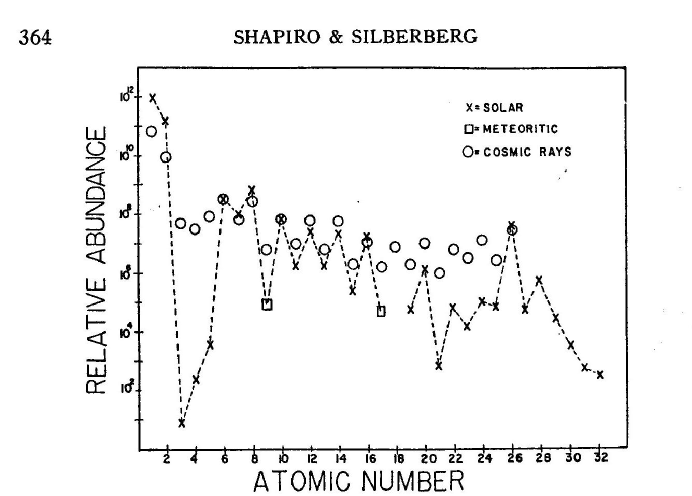
It is appropriate to begin this lecture with a diagram from the review of [Shapiro & Silberberg, 1970], which compares the abundances of elements in the cosmic radiation with solar system abundances. This classic measurement is one of the foundations of cosmic-ray physics. The elements lithium, beryllium and boron are quite abundant among cosmic rays even though they constitute only a tiny fraction of the material in the solar system and the interstellar medium. This fact is understood largely as the result of spallation of the “primary” nuclei carbon and oxygen during their propagation in the interstellar medium. The idea is that the protons and nuclei are accelerated from the interstellar medium and/or from the gas in or near their sources. The composition of the “primary” nuclei (defined as those initially accelerated and injected into the interstellar medium with high energy) reflects the combination of nuclei present in the material that is accelerated, which contains negligible amounts of “secondary” elements such as Li, Be, B. These secondary nuclei are fragmentation products of heavier primary nuclei.
In this picture, the amount of secondary nuclei is a measure of the characteristic time for propagation of cosmic rays before they escape from the galaxy into inter-galactic space. A simplified version of the diffusion equation that relates the observed abundances and spectra to initial values is
| (1) |
Here is the spatial density of cosmic-ray nuclei of mass , and is the number density of target nuclei (mostly hydrogen) in the interstellar medium, is the number of primary nuclei of type accelerated per cm3 per second, and and are respectively the total and partial cross sections for interactions of cosmic-ray nuclei with the gas in the interstellar medium. The second term on the r.h.s. of Eq. 1 represents losses due to interactions with cross section and decay for unstable nuclei with lifetime . The energy per nucleon, , remains constant to a good approximation in the transition from parent nuclei to nuclear spallation products, which move with velocity and Lorentz factor .
A crude first estimate of the characteristic diffusion time can be made by neglecting propagation losses for a primary nucleus and assuming that for a secondary nucleus . If we also neglect collision losses by the secondary nucleus after it is produced, then the solution of Eq. 1 is
| (2) |
Since the density in the disk of the galaxy is of order one particle per cm3 and the typical partial cross section for a light nucleus will be of order mb, the scale for the characteristic time is years. The full analysis requires self-consistent solution of the coupled equations for all species accounting for all loss terms, as described in John Wefel’s lecture in this volume ([Wefel, 2005]). A nice overview of propagation models is given by [Jones et al., 2001].
The thickness of the disk of the galaxy is of order 300 pc = 1000 light years, which is much shorter than the characteristic propagation time of 10 million years. The explanation is that the charged particles are trapped in the turbulent magnetized plasma of the interstellar medium and only diffuse slowly away from the disk, which is assumed to be where the sources are located. Measurements of the ratio of unstable to stable secondary nuclei (especially ) are used to determine independently of the product and hence to constrain further the models of cosmic-ray propagation.
Another important fact is that the ratio is observed to decrease with energy. From Eq. 2 this implies that also decreases. Simple power-law fits to ratios like B/C give
| (3) |
with . This behavior has important consequences for the source spectrum. To see this, consider an abundant, light primary nucleus such as hydrogen or helium. They are sufficiently abundant so that feed-down from heavier nuclei can be neglected and their cross sections are small enough so that energy losses in the interstellar medium can also be neglected in a first approximation. Then Eq. 1 reduces to
| (4) |
The local energy-density spectrum of cosmic rays is related to the observed flux (particles per cm2 per GeV per second per steradian) by
| (5) |
Since with the inference is that the cosmic accelerators are characterized by a power law with spectral index . This value is close to the spectral index for first order acceleration by strong shocks in the test-particle approximation ([Ostrowski, 2005]).
If the time for diffusion out of the galaxy continues to be described by to very high energy there is a problem: as decreases and approaches galactic scales, the cosmic-ray fluxes should become significantly anisotropic, which is not observed. One possibility is that the observed energy-dependence at low energy is due to a combination of “reacceleration” ([Seo & Ptuskin, 1994, Heinbach & Simon, 1995]) by weak shocks in the interstellar medium after initial acceleration by strong shocks. In such models, the high-energy behavior of diffusion is typically described by a slower energy dependence with . If so, the source spectral index would be steeper, approximately . In any case, in more realistic non-linear treatments of acceleration by strong shocks, the spectrum has some curvature, being steeper at low energy and harder at the high energy end of the spectrum ([Berezhko & Ellison, 1999]). What we observe may be some kind of average over many sources, each of which is somewhat different in shape and maximum energy.
The assumption underlying the discussion above is that the sources accelerating cosmic rays are in the disk of the galaxy and that the energy density in cosmic rays observed locally is typical of other regions of the galactic disk. If so, the total power required to maintain the cosmic radiation in equilibrium may be obtained by integrating Eq. 4 over energy and space. The result is
| (6) |
Using the observed spectrum and the value of explained above, one finds numerically
| (7) |
The kinetic energy of an expanding supernova remnant is initially of order erg, excluding the neutrinos, which carry away most of the energy released but do not disturb the interstellar medium. There are perhaps 3 supernovae per century, which gives erg/s as an estimate of the power which is dissipated in the interstellar medium by means of strong shocks driven by supernova ejecta. These are just the ingredients needed for acceleration of galactic cosmic rays. I return to the subject of cosmic-ray acceleration in §3 below.
2 Secondary cosmic-rays
Depending on the context, the term secondary cosmic rays can refer either to particles produced by interactions of primary cosmic rays with the interstellar gas or to particles produced by interactions of cosmic rays in the Earth’s atmosphere. The production mechanisms are similar, and there are some common features.
We have already seen one example, the secondary nuclei produced by occasional interactions of primary cosmic-ray nuclei during their propagation in the interstellar medium. In that case, to a good approximation, the energy per nucleon of the secondary nucleus is the same as that of the parent nucleus. The reason is that the nuclear fragments are only spectators to any production of secondary pions that may occur in the collisions. In general, however, the production term (last term of Eq. 1) will involve an integration over the energy of the parent particle. The main process to consider is production of pions by interaction of protons with a target nucleus. The production spectrum of the pions is
| (8) |
Here is the interaction length of protons in a medium consisting of nuclei of mass , and d is the differential element of mass traversed in distance d in a medium of density . It is often a useful approximation at high energy (i.e. energy particle masses) to assume a scaling form for the dimensionless production spectrum:
| (9) |
The scaling variable is , and Eq. 8 becomes
| (10) |
The last step on the r.h.s. of Eq. 10 follows when the parent spectrum is a power law in energy (). In that case, in the high-energy scaling approximation
| (11) |
i.e. the energy spectrum of secondaries has the same power behavior as the primaries scaled down by a factor
| (12) |
The spectrum-weighted moment depends both on the physics of production of the secondary pion and on the value of the differential spectral index .
2.1 Galactic secondaries
2.1.1 Diffuse gamma-rays
Gamma-ray emission from the disk of the galaxy is a powerful probe of the model of cosmic-ray origin and propagation as well as of the structure of the galaxy. Unlike charged cosmic rays, secondary photons propagate in straight lines. Since the galaxy is transparent for -rays of most energies, it is possible to search for concentrations of primary cosmic-ray activity from the map of the -ray sky after subtracting point sources. For example, if cosmic-ray acceleration is correlated with regions of higher density such as star-forming regions where supernovae are more frequent, then one would expect a quadratic enhancement of secondary production because of the spatial correlation between primary flux and target density.
The baseline calculation is to assume that the intensity observed locally at Earth is representative of the distribution everywhere in the disk of the galaxy. One can then look for interesting variation superimposed on this baseline. Following the analysis of Eqs. [9,10,11,12], the average number of neutral pions produced per GeV per unit volume in the interstellar medium is
| (13) |
Next this expression has to be convolved with the distribution of photons produced in . In the rest frame of the parent pion, each photon has MeV. The angular distribution is isotropic, so
| (14) |
where is the polar angle of the photon along the direction of motion of the parent pion but evaluated in the rest frame of the pion. For decay in flight of a pion with Lorentz factor and velocity , the energy of each of the resulting photons is
| (15) |
with for the two photons. Changing variables in Eq. 14 then gives
| (16) |
For the convolution of the distribution (16) with the production spectrum of neutral pions (13) gives
| (17) |
Numerically, in the approximation of uniform cosmic-ray density and uniform gas density in the interstellar medium, the observed gamma-ray flux would be
| (18) |
Here is the distance in a direction to the effective edge of the galactic disk, where and are galactic latitude and longitude. The effective distance is defined with respect to an equivalent disk of uniform density. Eq. 18 compares well in order of magnitude with the measured intensity of GeV photons by Egret ([Hunter et al., 1997]). The derivation of Eq. 18 is grossly oversimplified compared to the actual model calculation made in the paper of [Hunter et al., 1997] of the diffuse, galactic gamma-radiation. The reader is urged to consult that paper to understand the impressive level of detail at which the data are understood. It is also interesting to compare Eq. 18 to the TeV diffuse flux measured by Milagro ([Goodman, 2005]).
The implication of Eq. 17 is that for MeV the diffuse gamma-ray spectrum should have the same power law behavior as the proton spectrum, . What is observed, however, is that the spectrum of gamma-rays from the inner galaxy is harder than this, having a power-law behavior of approximately ([Hunter et al., 1997]). This is currently not fully understood. One possibility is that the cosmic-ray spectrum producing the gamma rays is harder than observed locally near Earth ([Hunter et al., 1997]).
Cosmic-ray electrons also contribute to the diffuse gamma-radiation by bremsstrahlung and by inverse Compton scattering. Fitting the observed spectrum requires a complete model of propagation that includes all contributions ([Hunter et al., 1997]). The distinguishing feature of -decay photons is a kinematic peak at . The origin of this feature can be seen in Eq. 15 from which the limits on for any given Lorentz factor of the parent pion are
The distribution is flat between these limits for each and is always centered around when plotted as a function . The individual contributions for parent pions of various energies always overlap at , so the full distribution from any spectrum always peaks at this value ([Stecker, 1971]).
2.1.2 Antiprotons and positrons
Antiprotons and positrons are of special interest because an excess over what is expected from production by protons during propagation could reflect an exotic process such as evaporation of primordial black holes or decay of exotic relic particles ([Bottino et al., 1998]). At a more practical level, they are important because they are secondaries of the dominant proton component of the cosmic radiation. As a consequence their spectra and abundances provide an independent constraint on models of cosmic-ray propagation ( [Moskalenko et al., 1998]).
Secondary antiprotons have a kinematic feature analogous to that in -decay gamma rays but at a higher energy related to the nucleon mass. In this case the feature is related to the high threshold for production of a nucleon-antinucleon pair in a proton-proton collision. This kinematic feature is observed in the data ([Orito et al., 2000]), and suggests that an exotic component of antiprotons is not required. Antiproton fluxes are consistent with the basic model of cosmic-ray propagation described in the Introduction.
Positrons are produced in the chain
Secondary electrons are produced in the charge conjugate process, but their number in the GeV range is an order of magnitude lower than primary electrons (i.e. electrons accelerated as cosmic rays). Because of radiative processes, the spectra of positrons and electrons are more complex to interpret than high-energy secondary -rays ([Moskalenko & Strong, 1998]). The measured intensity of positrons appears to be consistent with secondary origin ([DuVernois et al., 2001]).
2.1.3 -rays and from young supernova remnants
The same equations that govern production of secondaries in the interstellar medium also apply to production in gas concentrations near the sources. For example, a supernova exploding into a dense region of the interstellar medium ([Berezhko & Völk, 2000]) or into the gas generated by the strong pre-supernova wind of a massive progenitor star ([Berezhko, Pühlhofer & Völk, 2003]) would produce secondary photons that could show up as point sources.
Indeed, for many years, observation of -decay -rays from the vicinity of shocks around young supernova remnants (SNR) has been considered a crucial test of the supernova model of cosmic-ray origin ([Drury et al., 1994]; [Buckley et al., 1998]). Note, however, that a sufficiently dense target is required. Moreover, it is difficult to distinguish photons from decay from photons originating in radiative processes of electrons ( [Gaisser, Protheroe & Stanev, 1998]). There are two signatures: at low energy, observation of a shoulder reflecting the peak at 70 MeV would be conclusive. At higher energy one has to depend on the hardness and shape of the spectrum for evidence of hadronic origin of the photons. (See [Drury et al., 2001] for a current review.)
Observation of high-energy neutrinos would be strong evidence for acceleration of a primary beam of nucleons because such neutrinos are produced in hadronic interactions. Expected fluxes are low ([Gaisser, Halzen & Stanev, 1995]), so large detectors are needed ([Montaruli, 2003, Migneco, 2005]).
2.2 Atmospheric secondaries
Production of secondary cosmic rays and -rays in the interstellar medium generally involves less than one interaction per primary. In the language of accelerators, this is the thin-target regime. In contrast, the depth of the atmosphere is more than ten hadronic interaction lengths, so we have a thick target to deal with. The relevant cascade equation is
where
The equation describes the longitudinal development of the components of the atmospheric cascade in terms of slant depth (dd) along the direction of the cascade.
The loss terms on the r.h.s. of Eq. 2.2 represent interactions and decay, in analogy to Eq. 1. Here
| (20) |
is the Lorentz dilated decay length of particle in g/cm3. The expression defines a critical energy below which decay is more important than re-interaction. Because the density of the atmosphere varies with altitude, it is conventional to define the critical energy at the depth of cascade maximum ([Gaisser, 1990]). For pions the critical energy in the terrestrial atmosphere is GeV, while GeV. In astrophysical settings, the density is usually low enough so that decay always dominates over hadronic interactions. An intermediate case of some interest is production of secondary cosmic rays in the solar chromosphere, where the scale height is larger than in the Earth’s atmosphere so that decay remains dominant for another order of magnitude ([Seckel, Stanev & Gaisser, 1991]).
The same set of cascade equations (see Eq. 2.2) governs air showers and uncorrelated fluxes of particles in the atmosphere. The boundary condition for an air shower initiated by a primary of mass and total energy is
| (21) |
and for all other particles. This approximation, in which a nucleus is treated as consisting of independently interacting nucleons, is called the superposition approximation. In practice in Monte Carlo solutions of the cascade equation it is straightforward to remove this approximation given a model of nuclear fragmentation, (e.g. [Battistoni, et al., 1997]).
The other important boundary condition is that for uncorrelated fluxes in the atmosphere:
| (22) |
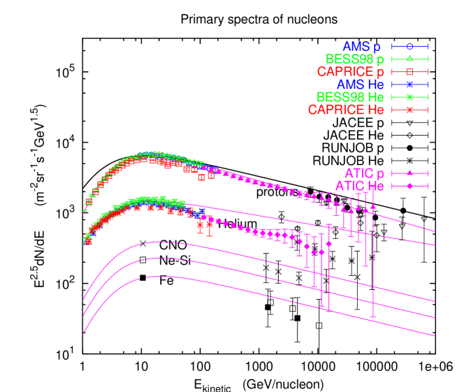
The numerical approximation is for the flux of all nucleons summed over the five major nuclear groups shown in Fig. 2. In Eq. 22, is total energy per nucleon. This numerical approximation is shown as the heavy solid line in Fig. 2. Its curvature at low energy is just a consequence of plotting the power law in total energy per nucleon as a function of kinetic energy per nucleon. Only a subset of available data is shown in Fig. 2. Data from the magnetic spectrometers BESS98 ([Sanuki, et al., 2000]) and AMS ([Alcarez et al., 2000a]) are indistinguishable on the plot for protons, although they differ somewhat for helium ([Alcarez et al., 2000b]). Data from the CAPRICE spectrometer ([Boezio et al., 1999]) are 15-20% lower than BESS98 above 10 GeV/nucleon. The higher energy data are from balloon-borne emulsion chambers, which are subject to larger systematic errors because not all energy is sampled in the calorimeter. Proton and helium data from JACEE ([Asakimori et al., 1998]) are shown. Data of RUNJOB ([Apanasenko et al., 2001]; [Furukawa et al., 2003]) are shown for five groups of nuclei (protons and helium, CNO, Ne-Si and Fe) above 1000 GeV. The fits to CNO, Ne-Si and Fe are normalized at 10.6 GeV/nucleon to data of [Engelmann et al., 1990].

2.2.1 Uncorrelated fluxes in the atmosphere
The simplest physical example to illustrate the solution of Eq. 22 is to calculate the vertical spectrum of nucleons as a function of depth in the atmosphere. Nucleons are stable compared to the transit time through the atmosphere, so only losses due to interactions are important in the cascade equation 2.2. In the approximation of scaling, the dimensionless distribution as in Eq. 9, with . Eq. 2.2 becomes
| (23) |
The dependence on energy and depth can be factorized, and the solution of Eq. 23 is
| (24) |
where the boundary condition 22 is satisfied if and . The attenuation length is related to the interaction length by
| (25) |
where is the spectrum-weighted moment for nucleons, analogous to Eq. 12 for pions.
The solution outlined above has several obvious approximations such as neglect of nucleon-anti-nucleon production and neglect of energy-dependence of the cross sections, but it nevertheless gives a reasonable representation of measurements of the spectrum of protons at various atmospheric depths, as shown in Fig. 3. For comparison with measurements of protons, the solution of Eq. 24 for all nucleons must be modified to remove neutrons, which increase slightly as a fraction of the total flux of nucleons with increasing depth in the atmosphere. The correction, as described in [Gaisser, 1990], is included in the calculations shown in Fig. 3.
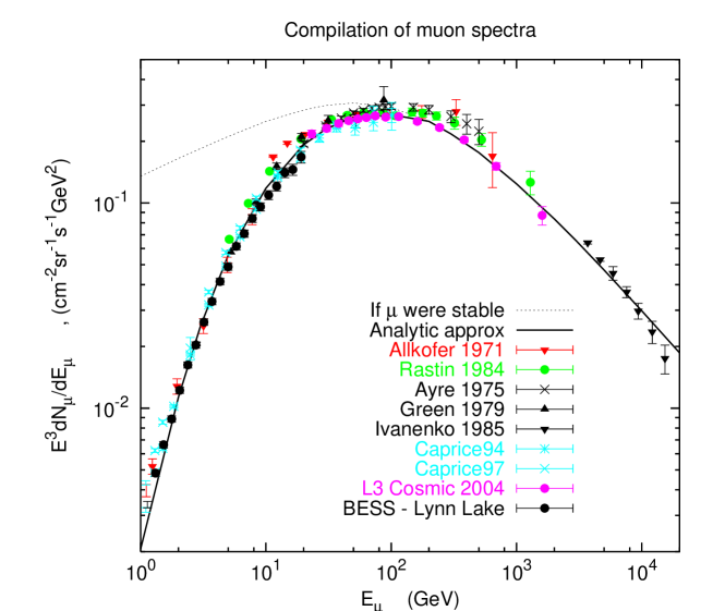
Another benchmark measurement of secondary cosmic rays in the atmosphere is the flux of muons. The main source of muons is from decay of charged pions. There is also a small contribution from decay of charged kaons, which becomes somewhat more important at high energy. At very high energy the muon energy spectrum becomes one power steeper than the parent spectrum of nucleons as a consequence of the extra power of in the ratio , which represents the decreasing probability of decay relative to re-interaction for charged pions at high energy (see Eqs. 2.2 and 20). For essentially all pions decay, and the muon production spectrum has the same power behavior as the parent pion and grandparent nucleon spectrum (). At low energy, however, muon energy-loss and decay become important, and the muon spectrum at the ground falls increasingly below the production spectrum. To account for all the complications one generally resorts to Monte Carlo calculations. However, analytic approximations ([Lipari, 1993]) of these effects are also possible. The full line in fig. 4 shows one such calculation ([Gaisser, 2002]), which uses as input the simple power-law primary spectrum of Eq. 22. This simple result compares relatively well to various measurements in several energy ranges. The recent data are from CAPRICE ([Kremer et al., 1999]), L3-Cosmic ([Achard et al., 2004]) and BESS ([Motoki et al., 2003]). One can also see the level of relative systematic uncertainties between different measurements.
Although I will not discuss the subject here, The most important secondary cosmic-ray flux is the atmospheric neutrino beam because of the discovery of neutrino oscillations by Super-Kamiokande ([Fukuda et al., 1998]). The experimental situation is reviewed by [Kajita & Totsuka, 2001] and [Jung et al., 2001], and the calculations by [Gaisser & Honda, 2002].
2.2.2 Air Showers
Above about 100 TeV cascades generated by individual primary nuclei have a big enough footprint deep in the atmosphere to trigger an array of widely spaced detectors on the ground. The threshold energy may be somewhat lower for closely spaced detectors, especially at high altitude. The threshold also may be made much higher by separating the detectors by a large distance. Examples of the latter are the Akeno Giant Air Shower Array (AGASA) ([Takeda et al., 2003]) and the surface detector of the Auger Project ([Watson et al., 2004]). Such ground arrays work by looking for coincidences in an appropriate time window, then reconstructing the primary direction and energy from the timing pattern of the hits and the size of the signals in the detectors. There are large fluctuations from shower to shower which complicate the interpretation of the data. The air shower technique is used at very high energy where the flux is too low to accumulate meaningful statistics with detectors carried aloft by balloons or spacecraft. The dividing line at present is approximately TeV.
Because of the complicated cascade of interactions that intervenes between the primary cosmic-ray nucleus incident on the atmosphere and the sparse data on the ground, Monte Carlo simulations are used to interpret the data. The other important reason for the necessity of a Monte Carlo generation of showers is that the detectors only sample a tiny fraction of the particles in the shower. Simulation of the response of an air shower detector to showers is therefore crucial. The standard, fully stochastic, four-dimensional air shower generator is CORSIKA ( [Heck & Knapp, 2003]). A cascade generator of similar scope and design is AIRES ([Sciutto, 2001]). A fast, one-dimensional cascade generator ([Alvarez-Muñiz et al., 2002]) that uses libraries of pre-generated subshowers at intermediate energies inside cascades is useful for analysis of ultra-high energy showers measured by fluorescence detectors for which knowledge of the lateral distribution is less important. The three-dimensional hybrid generator SENECA ([Drescher & Farrar, 2003]) uses stochastic Monte Carlo methods for the high-energy part of the shower and at the detector level, but saves time by numerically integrating the cascade equations for intermediate energies. The FLUKA program ( [Fassò et al., 2001]) is a general code for transport and interaction of particles through detectors of various types, including a layered representation of the atmosphere. The FLUKA interaction model ([Battistoni et al., 2004]) is built into the code and cannot be replaced by a different event generator.
There is a variety of hadronic event generators on the market ([Bopp et al., 2004, Kalmykov et al., 1997, Engel et al., 2001, Werner, 1993, Bossard et al., 2001]), which can be called by cascade programs like CORSIKA or AIRES to generate showers. Because the event generators are based on interpolations between measurements with accelerators at specific points in phase space and because the energies involved require extrapolations several orders of magnitude beyond those accessible with present accelerators, different hadronic event generators give different results for observables in air showers. We will see examples of this in the discussion of air showers below.
An air shower detector essentially uses the atmosphere as a calorimeter. Each shower dissipates a large fraction of its energy as it passes through the atmosphere, which is sampled in some way by the detector. It is therefore customary to plot the energy spectrum in the air shower regime by total energy per particle rather than by energy per nucleon as at low energy. In the lower energy regime the identity of each primary nucleus can be determined as it passes through the detector on a balloon or spacecraft. With air showers one has to depend on Monte Carlo simulations to relate what is measured to the primary energy and to the mass of the primary particle. The resulting energy assignments typically have uncertainties 20-30%. Primary mass is often quoted as an average value for a sample of events in each energy bin, or at best as a relative fraction of a small number of groups of elements.
3 Acceleration
A detailed review of the theory of particle acceleration by astrophysical shocks is given in the lectures of [Ostrowski, 2005]. The main feature necessary for understanding the implications of air shower data for origin of high-energy cosmic rays is the concept of maximum energy. Diffusive, first-order shock acceleration works by virtue of the fact that particles gain an amount of energy at each cycle, where a cycle consists of a particle passing from the upstream (unshocked) region to the downstream region and back. At each cycle, there is a probability that the particle is lost downstream and does not return to the shock. Higher energy particles are those that remain longer in the vicinity of the shock and have time to achieve high energy.
After a time the maximum energy achieved is
| (26) |
where refers to the velocity of the shock. This result is an upper limit in that it assumes a minimal diffusion length equal to the gyroradius of a particle of charge in the magnetic fields behind and ahead of the shock. Using numbers typical of Type II supernovae exploding in the average interstellar medium gives TeV ( [Lagage & Cesarsky, 1983]). More recent estimates give a maximum energy larger by as much as an order of magnitude or more for some types of supernovae ([Berezhko, 1996]).
The nuclear charge, , appears in Eq. 26 because acceleration depends on the interaction of the particles being accelerated with the moving magnetic fields. Particles with the same gyroradius behave in the same way. Thus the appropriate variable to characterize acceleration is magnetic rigidity, , where is the total momentum of the particle. Diffusive propagation also depends on magnetic fields and hence on rigidity. For both acceleration and propagation, therefore, if there is a feature characterized by a critical rigidity, , then the corresponding critical energy per particle is .
4 The anatomy of the cosmic-ray spectrum
The knee of the spectrum is the steepening that occurs above eV, as shown in Fig. 5, while the ankle is the hardening around eV. One possibility is that the knee is associated with the upper limit of acceleration by galactic supernovae, while the ankle is associated with the onset of an extragalactic population that is less intense but has a harder spectrum that dominates at sufficiently high energy. The general idea that the knee may signal the end of the population of particles produced in the Galaxy is an old one that I will trace in the next two subsections.
4.1 The knee
If the knee is a consequence of galactic cosmic accelerators reaching their limiting energy, then there are consequences for energy-dependence of the composition that can be used to check the idea. This follows from the form of Eq. 26. Consider first the simplest case in which all galactic accelerators are identical. Then , where characterizes the maximum rigidity. When the particles are classified by total energy per nucleus, protons will cut off first at , helium at , etc. [Peters, 1961] described this cycle of composition change and pointed out the consequences for composition in a plot like that reproduced here as Fig. 6. Since the abundant elements from protons to the iron group cover a factor of 30 in , the “Peters cycle” should occupy a similar range of total energy.
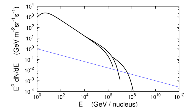
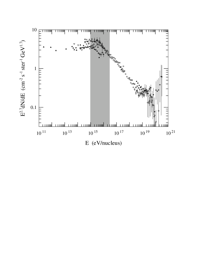
Because the observed spectrum does not abruptly stop, Peters hypothesized a new population of particles coming in with a somewhat harder spectrum, as indicated by the line in Fig. 6. Comparison with the data in Fig. 5 shows that reality is more complicated. The shaded area indicates the factor of 30 for a Peters cycle assuming eV. What is observed is that the steepened spectrum above the knee continues on smoothly for more than an order of magnitude in energy before any sign of a hardening. Even postulating a significant contribution from elements heavier than iron (up to uranium, [Hörandel, 2004]) cannot explain the smooth continuation all the way up to the ankle.
One possibility is that most galactic accelerators cut off around a rigidity of perhaps eV, but a few accelerate particles to much higher energy and account for the region between the knee and the ankle ([Erlykin & Wolfendale, 2001]). This scenario would be a generalization of Peters’ model. Its signature would be a sequence of composition cycles alternating between light and heavy dominance as the different components from each source cut off. As emphasized by [Axford, 1994], however, the problem with this type of model is that it requires a fine-tuning of the high-energy spectra so that they rise to join smoothly at the knee then steepen to fit the data to eV. As a consequence, several models have been proposed in which the lower-energy accelerators ( eV) inject seed particles into another process that accelerates them to higher energy. In this way the spectrum above the knee is naturally continuous with the lower energy region. One such possibility is acceleration by interaction with multiple supernova shocks in a cluster of supernovae ([Axford, 1994]). Another possibility ([Völk & Zirakashvili, 2003]) is acceleration by a termination shock in the galactic wind ([Jokipii & Morfill, 1987]).
The fine tuning problem (i.e. to achieve a smooth spectrum with a sequence of sources with different maxima) was actually clearly recognized by [Peters, 1961] in his original statement of this idea. He correctly pointed out, however, that since the cutoff is a function of rigidity while the events are classified by a quantity close (but not equal) to total energy, the underlying discontinuities are smoothed out to some extent. An interesting question to ask in this context is what power at the source would be required to fill in the spectrum from the knee to the ankle. The answer depends on what is assumed for the spectrum of the sources and the energy dependence of propagation in this energy region. Reasonable assumptions (e.g. and with ) lead to an estimate of erg/s, less than 10% of the total power requirement for all galactic cosmic-rays. For comparison, the micro-quasar SS433 at 3 kpc distance has a jet power estimated as erg/s ([Distefano et al., 2002]).
Another possibility is that the steepening of the spectrum at the knee is a result of a change in properties of diffusion in the interstellar medium such that above a certain critical rigidity the characteristic propagation time decreases more rapidly with energy. If the underlying acceleration process were featureless, then the relative composition as a function of total energy per particle would change smoothly, with the proton spectrum steepening first by , followed by successively heavier nuclei. It is interesting that this possibility was also explicitly recognized by [Peters, 1961].
A good understanding of the composition would go a long way toward clarifying what is going on in the knee region and beyond. A recent summary of direct measurements of various nuclei shows no sign of a rigidity-dependent composition change up to the highest energies accessible ( eV/nucleus) ([Battiston, 2004]). The change associated with the knee is in the air shower regime. Because of the indirect nature of EAS measurements, however, the composition is difficult to determine unambiguously. The composition has to be determined from measurements of ratios of different components of air showers at the ground. For example, a heavy nucleus like iron generates a shower with a higher ratio of muons to electrons than a proton shower of the same energy. [Swordy et al., 2002] reviewed all available measurements of the composition at the knee. A plot of mean log mass () ([Ahrens et al., 2004b]) shows no clear pattern when all results are plotted together. The best indication at present comes from the Kascade experiment ( [Roth, 2003]), which shows clear evidence for a “Peters cycle”, the systematic steepening first of hydrogen, then of helium, then CNO and finally the iron group. The transition occurs over an energy range from approximately eV to eV, as expected, but the experiment runs out of statistics by eV, so the data do not yet discriminate among the various possibilities for explaining the spectrum between the knee and the ankle.
4.2 The ankle
Above some sufficiently high energy it seems likely that the cosmic rays will be of extra-galactic origin. A proton of energy eV has a gyroradius of a kiloparsec in a typical galactic magnetic field, which is larger than the thickness of the disk of the Galaxy. Given constraints from observed isotropy of particles with eV, where the corresponding proton gyroradius is comparable to the full extent of the Galaxy, the usual assumption is that particles above originate outside our galaxy. There is a suggestion of an anisotropy just around eV from the central regions of the galaxy ([Hayashida et al., 1999]) that may be due to neutrons, which survive for a mean pathlength of kpc at this energy, and could therefore reach us from the galactic center. If so, this would suggest that at least some fraction of the cosmic rays around eV are still of galactic origin. An interesting discussion of possible implications is given by [Anchordoqui et al., 2004a]. In any case, the questions of whether there is a transition from galactic to extragalactic cosmic rays and at what energy such a transition occurs are of great interest.

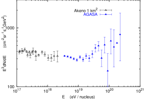

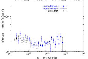
As background for a discussion of the significance of the ankle and how it should be interpreted, it is helpful to look at the spectrum from individual measurements separately so that systematic differences between measurements do not obscure any details that may be present. Results from four groups are shown in Fig. 7: Fly’s Eye stereo ([Bird, et al., 1993]); Akeno ([Nagano et al., 1992]) and AGASA ([Takeda et al., 2003]); Yakutsk ([Glushkov et al., 2003]); and the measurements made with Hi-Res ([Abassi et al., 2004] and [Abu-Zayyad et al., 2001]). In all these measurements there is a suggestion of a steepening just below eV, which is sometimes referred to as the “second knee.” The ankle appears as a saddle-like shape with its low point between and eV, depending on the experiment. One could fit the saddle with a final Peters cycle starting just below eV and an extragalactic component crossing as in Fig. 6 to contribute to the ankle in the overall spectrum ([Bahcall & Waxman, 2003]). Alternatively, it is possible to make a model in which extragalactic cosmic rays account for the entire observed flux down to eV ([Berezinsky et al., 2004]) or even lower ( [Bergman, 2004]). The difference lies in the assumptions made for the spectrum and cosmological evolution of the sources. I will return to this issue in the next section.
First it is interesting to ask what data on primary composition may tell us about the changing populations of particles above eV. In this energy range the composition is measured by the energy dependence of the position of shower maximum, . An air shower consists of a superposition of electromagnetic cascades initiated by photons from decay of particles produced by hadronic interactions along the core of the shower as it passes through the atmosphere. Most of the energy of the shower is dissipated by ionization losses of the low-energy electrons and positrons in these subshowers. The composite shower reaches a maximum number of particles (typically particles per GeV of primary energy) and then decreases as the individual photons fall below the critical energy for pair production. Because each nucleus of mass and total energy essentially generates subshowers each of energy the depth of maximum depends on . Since cascade penetration increases logarithmically with energy,
| (27) |
where is a parameter (the “elongation rate”) that depends on the underlying properties of hadronic interactions in the cascade.
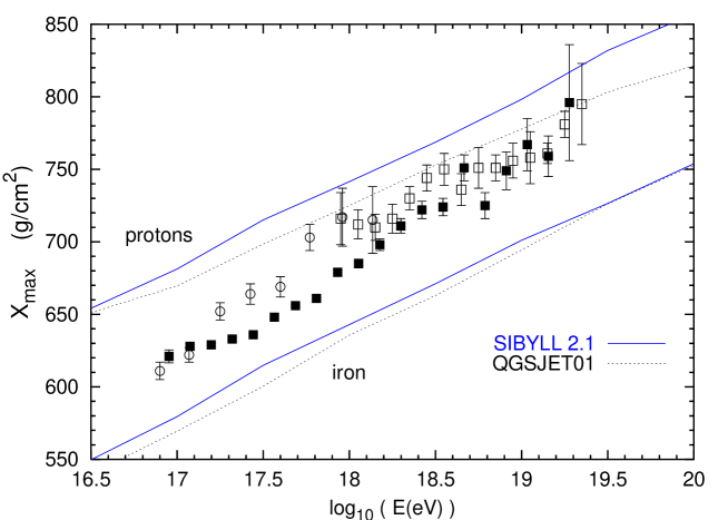
Fig. 8 shows results of measurements with the Fly’s Eye stereo detector ([Bird, et al., 1993]) compared to measurements of HiRes ([Abu-Zayyad et al., 2001]; [Archbold & Sokolsky, 2003]). A weak inference about composition can be made by comparing to the results of simulations, two of which are shown in the figure. Both calculations use CORSIKA ( [Heck & Knapp, 2003]) with two different interaction models ([Kalmykov et al., 1997, Engel et al., 2001]). The measurement with the Fly’s Eye Stereo detector suggests a transition from a large fraction of heavies below eV to a larger fraction of protons by eV (how much larger depending on which interaction model is chosen). The coincidence of the change of composition from heavier toward lighter) around eV with the ankle feature in the Fly’s Eye data at the same energy led to the suggestion of a transition from galactic to extragalactic cosmic rays as a possible explanation ([Bird, et al., 1993]). This interpretation would favor a model like that of [Bahcall & Waxman, 2003]. The more recent HiRes data set, however, shows the transition from heavier toward lighter beginning at eV and complete by eV, consistent with the models of [Berezinsky et al., 2004] and [Bergman, 2004].
Because of the uncertainties in the interaction models above accelerator energies coupled with statistical and systematic limitations of the experiments, the primary composition as a function of energy above eV remains an open question ([Watson, 2004]).
5 Highest energy cosmic rays
Protons lose energy by three loss processes during propagation through the cosmos. Red-shift losses (adiabatic losses due to expansion of the Universe), which apply to all particles, become important when the distance scales are comparable to the Hubble distance Gpc. Protons of sufficiently high energy also interact with the microwave background and lose energy to electron-positron pair production (for eV) and to photopion production (for eV). The corresponding attenuation lengths (for reducing energy by a factor ) are Gpc and Mpc, respectively. The photo-pion process leads to the expectation of a suppression of the flux above eV unless the sources are within a few tens of Mpc. The suppression is referred to as the GZK cutoff (or GZK feature) in recognition of the authors of the two papers, [Greisen, 1966] and [Zatsepin & Kuz’min, 1966] who first pointed out the effect shortly after the discovery of the microwave background radiation.
The actual shape of the spectrum at Earth after accounting for these three loss processes depends on what is assumed
-
•
for the spatial distribution of sources,
-
•
for the spectrum of accelerated particles at the sources, and
-
•
for the possible evolution of activity of the sources on cosmological time scales.
A classic calculation is that of [Berezinsky & Grigorieva, 1988], in which the energy-loss equation is integrated numerically. This approach neglects effects of fluctuations, which may be noticeable in certain circumstances. A recent example of a Monte Carlo propagation calculation of cosmological propagation is by [Stanev et al., 2000], which contains comparisons with other calculations. Figure 9 from [Abassi et al., 2002] shows an example of a calculated cosmologically evolved spectrum compared to data of HiRes ([Abassi et al., 2004]) and AGASA ([Takeda et al., 2003]).
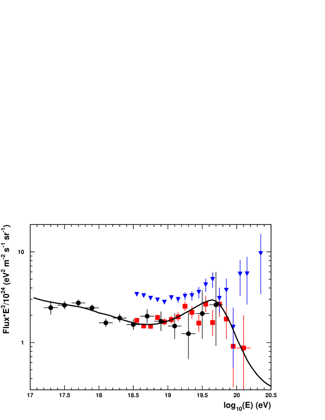
The calculation illustrated in Fig. 9 is for a uniform distribution of sources out to large red shifts. The “pile-up” (which is amplified by plotting differential flux) is populated by particles that have fallen below the GZK energy. The saddle or ankle feature on the plot is a consequence of energy losses to pair production. The data below eV have been fit in this example by adding an assumed galactic contribution, which is not shown separately here (but see [Bergman, 2004] for a discussion). As pointed out long ago by [Hillas, 1968] (see also [Hillas, 1974]), the degree to which the extragalactic flux contributes at low energy (for example below eV) can be adjusted by making different assumptions about increased activity at large redshift, z 1. Such high redshift sources do not contribute at high energy because of adiabatic losses, but they can contribute at low energy if they were sufficiently abundant. On the other hand, it is also possible to construct a model in which the extragalactic sources only contribute significantly at very high energy (e.g. above eV), as in [Bahcall & Waxman, 2003].
The question of the energy above which the extragalactic component accounts for all of the observed spectrum is important because it is directly related to the amount of power needed to supply the extragalactic component. An estimate of the power needed to supply the extragalactic cosmic rays is obtained by the replacements and in Eq. 6, where yrs is the Hubble time and is the extragalactic component of the total cosmic-ray flux. The result depends on where the EG-component is normalized to the total flux and on how it is extrapolated to low energy. A minimal estimate follows from taking the hardest likely spectral shape (differential index ) and normalizing at eV. This leads to a total power requirement of erg/Mpc3/s. If the rate of GRBs is 1000 per year, then they would need to produce erg/burst in accelerated cosmic rays to satisfy this requirement. The density of AGNs is ([Peebles, 1993]), so the corresponding requirement would be erg/s per AGN in accelerated particles. Normalizing the extragalactic component at eV increases the power requirement by a factor of 10, and assuming a softer spectral index increases it even more. These are very rough estimates just meant to illustrate the relation between the intensity of extragalactic cosmic rays and the power needed to produce them. A proper treatment requires an integration over redshift, accounting for the spatial distribution of sources and their evolution over cosmic time ([Stanev, 2003]).
In addition to being able to satisfy the power requirement, the sources also have to be able to accelerate particles to eV. The requirements on size and magnetic field in the sources are essentially given by setting eV in Eq. 26 and solving for the product of (or ). The resulting constraint on the sources is the famous plot of [Hillas, 1984]. Sites with a sufficiently large included active galactic nuclei (AGN) ([Berezinsky et al., 2004]) and the termination shocks of giant radio galaxies ([Biermann & Strittmatter, 1987]). Since 1984 two more potential candidates have emerged, jets of gamma-ray bursts (GRB [Waxman, 1995, Vietri, 1995]) and magnetars.
Neutrino telescopes may make a decisive contribution to identifying ultra-high energy cosmic accelerators by finding point sources of TeV neutrinos and associating them with known objects, for example with gamma-ray sources such as AGN or GRB. Even the detection of a diffuse flux of high-energy, extraterrestrial neutrinos, or the determination of good limits can constrain models of cosmic-ray origin under the assumption that comparable amounts of energy go into cosmic-rays and into neutrinos produced by the cosmic-rays at the sources ([Anchordoqui et al., 2004b]).
As is well-known, the AGASA measurement ([Takeda et al., 2003]) shows the spectrum continuing beyond the GZK energy without a suppression, while the HiRes measurement ([Abassi et al., 2004]) is consistent with the GZK shape. The discrepancy between the two experiments is not as great as it appears in Fig. 9. The difference is amplified quadratically when the differential spectrum is multiplied by in the plot. A 20-30% shift in energy assignment (downward for AGASA or upward for HiRes) brings the two data sets into agreement below eV. A quantitative estimate of the statistical significance of the difference above eV is ambiguous because it depends on what is assumed for the true spectrum. The difference is generally considered to be less than three sigma, however ([Olinto, 2004]). One of the first goals of the Auger project ([Klages, 2005]) is to resolve the question of whether the spectrum extends significantly beyond the GZK energy. If not, then higher statistics accumulated by Auger may be used to constrain models of extra-galactic sources by making precise measurements both above and below the GZK energy. If the spectrum does continue beyond the cutoff then identification of specific, cosmologically nearby sources from the directions of the ultra-high energy events would be likely.
6 Conclusion and outlook
While the questions surrounding the highest energy particles are clearly of the greatest importance, there are several important open questions at all energies. One is the transition, if it exists, from galactic to extra-galactic cosmic rays. Proposed experiments associated with the telescope array ([Arai et al., 2003]) may be optimized to provide good coverage down to eV ([Thompson, 2004]).
Understanding the knee of the spectrum remains an outstanding problem in cosmic-ray astrophysics. Kascade-Grande ([Huangs et al., 2003]) will cover the energy range from below the knee to eV with a multi-component air shower array at sea level. The IceCube detector at the South Pole ([Ahrens et al., 2004a]) will have a kilometer square surface component, IceTop ([Gaisser et al., 2003]; [Stanev, et al., 2005]), 1.4 km above the top of the cubic kilometer neutrino telescope. The whole constitutes a novel, large three-dimensional air shower detector with coverage of the cosmic-ray spectrum from below the knee to eV. In addition to its main mission of neutrino astronomy, IceCube therefore also has the potential to make important contributions to related cosmic-ray physics. The high altitude of the surface (9300 m.a.s.l.) allows good primary energy resolution with the possibility of determining relative importance of the primary mass groups from the ratio of size at the surface to muon signal in the deep detector. With a coverage extending to eV, these detectors also have the potential to clarify the location of a transition to cosmic-rays of extragalactic origin.
While the knee of the spectrum remains in the realm of air shower experiments for the time being, there is much activity aimed at extending direct measurements of the primary spectrum and composition to reach the knee from below. The detectors include Advanced Thin Ionization Calorimeter (ATIC, [Wefel et al., 2003]); Transition Radiation Array for Cosmic Energetic Radiation (TRACER, [Müller, 2005]); Cosmic Ray Energetics and Mass (CREAM, [Seo et al., 2003]) and Advanced Cosmic-ray Composition Experiment for Space Station (ACCESS, http://www.atic.umd.edu/access.html). While ACCESS is to be flown in space, ATIC, TRACER and CREAM all take advantage of NASA’s long-duration balloon program which is regularly achieving flights of two to four weeks in Antarctica. These experiments also have the opportunity to extend measurements of the ratio of secondary to primary nuclei to much higher energy and hence to resolve the related questions about the average source spectral index and about the isotropy of galactic cosmic rays.
References
- [Abassi et al., 2002] Abassi, R.U. et al. (2002). astro-ph/0208301.
- [Abassi et al., 2004] Abassi, R.U. et al. (2004). Phys. Rev. Letters, 92:151101.
- [Abu-Zayyad et al., 2001] Abu-Zayyad, T. et al. (2001). Ap.J., 557:686.
- [Achard et al., 2004] Achard, P. et al. (2004). Phys. Lett. B, 598:15.
- [Ahrens et al., 2004a] Ahrens, J. et al. (2004a). Astropart. Phys., 20:507.
- [Ahrens et al., 2004b] Ahrens, J. et al. (2004b). Astropart. Phys., 21:565.
- [Alcarez et al., 2000a] Alcarez, J. et al. (2000a) Phys. Lett. B, 490:27.
- [Alcarez et al., 2000b] Alcarez, J. et al. (2000b) Phys. Lett. B, 494:193.
- [Alvarez-Muñiz et al., 2002] Alvarez-Muñiz, J. et al. (2002). Phys. Rev. D, 66:033011.
- [Allkofer et al., 1971] Allkofer, O.C., Carstensen, K. & Dau, W.D. (1971). Phys. Lett. B, 36:425.
- [Anchordoqui et al., 2004a] Anchordoqui, L.A., Goldberg, H., Halzen, F. & Weiler, T.J. (2004). Phys. Lett. B, 593:42.
- [Anchordoqui et al., 2004b] Anchordoqui, L.A., Goldberg, H., Halzen, F. & Weiler, T.J. (2004). hep-ph/0410003.
- [Apanasenko et al., 2001] Apanasenko, A.V. et al. (2001). Astropart. Phys., 16:13.
- [Arai et al., 2003] Arai, Y. et al. (2003). in Proc. 28th Int. Cosmic Ray Conf. (Tsukuba, ed. T. Kajita et al., Universal Academy Press), 2:1025.
- [Archbold & Sokolsky, 2003] Archbold, G. & Sokolsky, P. (2003). in Proc. 28th Int. Cosmic Ray Conf. (ed. T. Kajita et al., Universal Academy Press) 1:405.
- [Asakimori et al., 1998] Asakimori, K. et al. (1998). Ap.J., 502:278.
- [Axford, 1994] Axford, W.I. (1994). Ap.J. Suppl., 90:937.
- [Ayre et al., 1975] Ayre, C.A. et al. (1975). J. Phys. G, 1:584.
- [Bahcall & Waxman, 2003] Bahcall, J.N. & Waxman, E. (2003). Phys. Lett. B, 556:1.
- [Battiston, 2004] Battiston, R. (2004). in Frontiers of Cosmic Ray Science (ed. T. Kajita et al., Universal Academy Press):229.
- [Battistoni, et al., 1997] Battistoni, G., Forti, C., Ranft, J. & Roesler, S. (1997). Astropart. Phys., 7:49.
- [Battistoni et al., 2004] Battistoni, G. et al. (2004). astro-ph/0412178
- [Berezhko, 1996] Berezhko, E.G. (1996). Astropart. Phys., 5:367.
- [Berezhko & Ellison, 1999] Berezhko, E.G. & Ellison, D.C. (1999). Ap.J., 526:385.
- [Berezhko & Völk, 2000] Berezhko, E.G. & Völk, H.J. (2000). Astropart. Phys., 14:201.
- [Berezhko, Pühlhofer & Völk, 2003] Berezhko, E.G., Pühlhofer, G. & Völk, H.J. (2003). Astron. Astrophys., 400:971.
- [Berezinsky & Grigorieva, 1988] Berezinsky, V.S. & Grigorieva, S.I. (1988). Astron. Astrophys., 199:1.
- [Berezinsky et al., 2004] Berezinsky, V., Gazizov, A. & Grigorieva, S. astro-ph/0410650.
- [Bergman, 2004] Bergman, D. (2004). astro-ph/0407244.
- [Biermann & Strittmatter, 1987] Biermann, P. & Strittmatter, P.A. (1987). Ap.J., 322:643.
- [Bird, et al., 1993] Bird, D.J. et al. (1993). Phys. Rev. Letters, 71:3401.
- [Boezio et al., 1999] Boezio, M et al. (1999). Ap.J., 518:457.
- [Bopp et al., 2004] Bopp, F.W., Ranft, J., Engel,, R. & Roesler, S. (2004). astro-ph/0410027 and references therein.
- [Bossard et al., 2001] Bossard, G. et al. (2001). Phys. Rev. D, 63:054030.
- [Bottino et al., 1998] Bottino, A. et al. (1998). Phys. Rev. D, 58:123503.
- [Buckley et al., 1998] Buckley, J.H. et al. (1998). Astron. Astrophys., 329:639.
- [Distefano et al., 2002] Distefano, C., Guetta, D., Waxman, E. & Levinson, A. Ap.J., 575:378.
- [Drescher & Farrar, 2003] Drescher, H.-J. & Farrar, G. (2003). Phys. Rev. D, 67:116001.
- [Drury et al., 1994] Drury, L.O’C., Aharonian, F.A. & Völk, H.J. (1994). Astron. Astrophys., 287:959.
- [Drury et al., 2001] Drury, L.O’C. et al. (2001). Ap. Sci. Rev., 99:329.
- [DuVernois et al., 2001] DuVernois, M.A. et al. (2001). Ap.J., 559:296.
- [Engel et al., 2001] Engel, R., Gaisser, T.K. & Stanev, Todor (2001). Proc. 27th Int. Cosmic Ray Conf. (ed. K.-H. Kampert, G. Heinzelmann & C. Spiering, Copernicus Gesellschaft, Hamburg) 2:431.
- [Engelmann et al., 1990] Engelmann, J.J. et al. (1990). Astron. Astrophys., 233:96.
- [Erlykin & Wolfendale, 2001] Erlykin, A.D. & Wolfendale, A.W. (2001). J. Phys. G, 27:1005.
- [Fassò et al., 2001] Fassò, A., Ferrari, A., Ranft, J. & Sala, P.R. (2001). in Proc. MonteCarlo 2000, Lisbon (ed. A. Kling et al., Springer-Verlag, Berlin):955.
- [Fukuda et al., 1998] Fukuda, Y. et al. (1998). Phys. Rev. Letters, 81:1562.
- [Furukawa et al., 2003] Furukawa, M. et al. (2003). in Proc. 28th Int. Cosmic Ray Conf. (Tsukuba, ed. T. Kajita et al., Universal Academy Press), 4:1837.
- [Gaisser, 1990] Gaisser, T.K. (1990). Cosmic Rays and Particle Physics (Cambridge University Press).
- [Gaisser, Halzen & Stanev, 1995] Gaisser, T.K., Halzen, F. & Stanev, Todor (1995). Phys. Reports, 258:173.
- [Gaisser, Protheroe & Stanev, 1998] Gaisser, T.K. Protheroe, R.J. & Stanev, Todor (1998). Ap.J., 492:219.
- [Gaisser, Honda, Lipari & Stanev, 2001] Gaisser, T.K., Honda, M., Lipari, P. & Stanev, Todor (2001). Proc. 27th Int. Cosmic Ray Conf. (Hamburg) 5:1643.
- [Gaisser, 2002] Gaisser, T.K. (2002). Astropart. Phys., 16:285.
- [Gaisser & Honda, 2002] Gaisser, T.K. & Honda, M. (2002). Ann. Revs. Nucl. Part. Sci., 52:153.
- [Gaisser et al., 2003] Gaisser, T.K. et al. (2003). in Proc. 28th Int. Cosmic Ray Conf. (Tsukuba, ed. T. Kajita et al., Universal Academy Press), 2:1117.
- [Gaisser & Stanev, 2004] Gaisser, T.K. & Stanev, Todor (2004). in S. Eidelman et al., Reviews of Particle Properties, Physics Letters B, 592:228.
- [Gaisser & Stanev, 2005] Gaisser, T.K. & Stanev, Todor (2005). Nucl. Phys. A:(to be published).
- [Glushkov et al., 2003] Glushkov, A.V. et al. (2003). in Proc. 28th Int. Cosmic Ray Conf. (Tsukuba, ed. T. Kajita et al., Universal Academy Press), 1:389.
- [Goodman, 2005] Goodman, Jordan (2005). This volume.
- [Green, 1979] Green, P.J. et al. (1979). Phys. Rev. D, 20:1598.
- [Greisen, 1966] Greisen, K. (1966). Phys. Rev. Letters, 16:748.
- [Hayashida et al., 1999] Hayashida, N. et al. (1999). Astropart. Phys., 10:303.
-
[Heck & Knapp, 2003]
Heck, D. & Knapp, J. (2003).
Extensive Air Shower simulation with CORSIKA: A user’s Guide,
(V 6.020, FZK Report, February 18, 2003).
http://www-ik.fzk.de/corsika/ - [Heinbach & Simon, 1995] Heinbach, U. & Simon, M. (1995). Ap.J., 441:209.
- [Hillas, 1968] Hillas, A.M. (1968). Canadian J. Phys., 46:S623.
- [Hillas, 1974] Hillas, A.M. (1974). Phil. Trans. R. Soc. Lond. A, 277:413.
- [Hillas, 1984] Hillas, A.M. (1984). Ann. Revs. Astron. Astrophys., 22:425.
- [Hörandel, 2004] Hörandel, J.R. (2004). Astropart. Phys., 21:241.
- [Huangs et al., 2003] Huangs, A. et al. (2003). in Proc. 28th Int. Cosmic Ray Conf. (Tsukuba, ed. T. Kajita et al., Universal Academy Press), 2:985.
- [Hunter et al., 1997] Hunter, S.D. et al. (1997). Ap.J., 481:205.
- [Ivanenko et al., 1985] Ivanenko, I.P. et al. (1985). in Proc. 19th Int. Cosmic Ray Conf., La Jolla (NASA Conf. Publ. No 2376) 8:21
- [Jokipii & Morfill, 1987] Jokipii, J.R. & Morfill, G.E. (1987). Ap.J., 312:170.
- [Jones et al., 2001] Jones, F.C., Lukasiak, A., Ptuskin, V. & Webber, W. (2001). Ap.J., 547:246.
- [Jung et al., 2001] Jung, C.K., Kajita, T., Mann, T. & McGrew, C. (2001). Ann. Rev. Nucl. Part. Sci., 51:451.
- [Kajita & Totsuka, 2001] Kajita, T. & Totsuka, Y. (2001). Revs. Mod. Phys., 73:85.
- [Kalmykov et al., 1997] Kalmykov, N.N., Ostapchenko, S.S. & Pavlov, A.I. (1997). Nucl. Phys. B (Proc. Suppl.), 52:17.
- [Klages, 2005] Klages, H. (2005). This volume.
- [Kremer et al., 1999] Kremer, J. et al. (1999). Phys. Rev. Letters, 83:4241.
- [Lagage & Cesarsky, 1983] Lagage, P.O. & Cesarsky, C.J. (1983). Astron. Astrophys., 118:223 and 125:249.
- [Lipari, 1993] Lipari, P. (1993). Astropart. Phys., 1:195.
- [Migneco, 2005] Migneco, E. (2005). This volume.
- [Mocchiutti, 2003] Mocchiutti, E. (2003). Atmospheric and Interstellar Cosmic Rays Measured with the CAPRICE98 Experiment (Thesis, KTH, Stockholm)
- [Montaruli, 2003] Montaruli, T. (2003). astro-ph/0312558 ( Nucl. Phys. B (Suppl.), to be published).
- [Moskalenko & Strong, 1998] Moskalenko, I.V. & Strong, A.W. (1998). Ap.J., 493:694.
- [Moskalenko et al., 1998] Moskalenko, I.V., Strong, A.W., Ormes, J.F. & Potgieter, M.S. (2002). Ap.J., 565:280.
- [Motoki et al., 2003] Motoki, M. et al. (2003). Astropart. Phys., 19:113.
- [Müller, 2005] Müller, D. (2005). This volume and http://tracer.uchicago.edu
- [Nagano et al., 1992] Nagano, M. et al. (1992). J. Phys. G, 18:423.
- [Olinto, 2004] Olinto, A. (2004). in Frontiers of Cosmic Ray Science (ed. T. Kajita et al., Universal Academy Press):299.
- [Orito et al., 2000] Orito, S. et al. (2000). Phys. Rev. Letters, 84:1078.
- [Ostrowski, 2005] Ostrowski, M. (2005). This volume.
- [Peebles, 1993] Peebles, P.J.E. (1993). Principles of Physical Cosmology (Princeton University Press).
- [Peters, 1961] Peters, B. (1961). Nuovo Cimento, XXII:800.
- [Rastin, 1984] Rastin, R.C. (1984). J. Phys. G, 10:1609.
- [Roth, 2003] Roth, M. et al. (2003). in Proc. 28th Int. Cosmic Ray Conf. (Tsukuba, ed. T. Kajita et al., Universal Academy Press), 1:139.
- [Sanuki, et al., 2000] Sanuki, T. et al. (2000). Ap.J., 545:1135.
-
[Sciutto, 2001]
Sciutto, S.J. (2001).
Proc. 27th
Int. Cosmic Ray Conf. (ed. K.-H. Kampert, G. Heinzelmann & C. Spiering,
Copernicus Gesellschaft, Hamburg) 1:237.
http://www.fisica.unlp.edu.ar/auger/aires/ - [Seckel, Stanev & Gaisser, 1991] Seckel, D. Stanev Todor & Gaisser, T.K. (1991). Ap.J., 382:651.
- [Seo & Ptuskin, 1994] Seo, E.S. & Ptuskin, V.S. (1994). Ap.J., 431:705.
- [Seo et al., 2003] Seo, E.-S. et al. (2003). in Proc. 28th Int. Cosmic Ray Conf. (Tsukuba, ed. T. Kajita et al., Universal Academy Press), 4:2101. http://cosmicray.umd.edu/cream/cream.html
- [Shapiro & Silberberg, 1970] Shapiro, Maurice M. & Silberberg, Rein (1970). Ann. Revs. Nucl. Sci., 20:323.
- [Stanev et al., 2000] Stanev, Todor et al. (2000). Phys. Rev. D, 62:093005.
- [Stanev, 2003] Stanev, Todor (2003). High Energy Cosmic Rays (Springer Verlag, Berlin).
- [Stanev, et al., 2005] Stanev, T. for the IceCube Collaboration (2005). astro-ph/0501046.
- [Stecker, 1971] Stecker, F.W. (1971). Cosmic Gamma Rays (NASA Scientific and Technical Information Office, NASA SP-249).
- [Swordy et al., 2002] Swordy, S. et al. (2002). Astropart. Phys., 18:129.
- [Takeda et al., 2003] Takeda, M. et al. (2003). Astropart. Phys., 19:447.
- [Thompson, 2004] Thompson, G. (2004). Talk given at Leeds Workshop on Ultra-High Energy Cosmic Rays, 22 July.
- [Vietri, 1995] Vietri, M. (1995). Ap.J., 453:883.
- [Völk & Zirakashvili, 2003] Völk, H.J. & Zirakashvili, V.N. (2003). in Proc. 28th Int. Cosmic Ray Conf. (Tsukuba, ed. T. Kajita et al., Universal Academy Press), 4:2031.
- [Watson et al., 2004] Watson, A.A. et al. (2004). Nucl. Inst. Methods A, 523:50.
- [Watson, 2004] Watson, A.A. (2004). astro-ph/0410514.
- [Waxman, 1995] Waxman, E. (1995). Phys. Rev. Letters, 75:386.
- [Wefel et al., 2003] Wefel, John et al. (2003). in Proc. 28th Int. Cosmic Ray Conf. (Tsukuba, ed. T. Kajita et al., Universal Academy Press), 4:1849.
- [Wefel, 2005] Wefel, John (2005). This volume.
- [Werner, 1993] Werner, K. (1993). Phys. Rep., 232:87.
- [Zatsepin & Kuz’min, 1966] Zatsepin, G.T. & Kuz’min, V.A. (1966). JETP Letters, 4:78.