Twenty-one centimeter tomography with foregrounds

Abstract

Twenty-one centimeter tomography is emerging as a powerful tool to explore the reionization epoch and cosmological parameters, but it will only be as good as our ability to accurately model and remove astrophysical foreground contamination. Previous treatments of this problem have focused on the angular structure of the signal and foregrounds and what can be achieved with limited spectral resolution (channel widths in the 1 MHz range). In this paper we introduce and evaluate a “blind” method to extract the multifrequency 21cm signal by taking advantage of the smooth frequency structure of the Galactic and extragalactic foregrounds. We find that 21 cm tomography is typically limited by foregrounds on scales $k\ll 1h/$Mpc and limited by noise on scales $k\gg 1h/$Mpc, provided that the experimental channel width can be made substantially smaller than 0.1 MHz. Our results show that this approach is quite promising even for scenarios with rather extreme contamination from point sources and diffuse Galactic emission, which bodes well for upcoming experiments such as LOFAR, MWA, PAST, and SKA.

1. Introduction

21 cm tomography is one of the most promising cosmological probes, with the potential to complement and perhaps ultimently eclipse the cosmological parameter constraints from the cosmic microwave background (Bowman et al., 2005; McQuinn et al., 2005). It is also a unique probe of the epoch of reionization, which is now one of the least understood aspects of modern cosmology. There are various techniques to explore the epoch of reionization at $5<z<20$. Apart from the CMB (Holder et al., 2003; Knox, 2003; Kogut et al., 2003; Santos et al., 2003), radio astronomical measurement of 21cm radiation from neutral hydrogen has been shown theoretically to be a powerful tool to study this period (Madau, Meiksin, & Rees, 1997; Tozzi et al., 2000). Lots of work has been done in recent years on various theoretical and experimental aspects of 21cm radiation (e.g., Barkana & Loeb, 2004a; Carilli, Gnedin, & Owen, 2002; Carilli et al., 2004a; Ciardi & Madau, 2003; DiMatteo et al., 2002; Dimatteo, Ciardi, & Miniati, 2004; Furlanetto, Sokasian, & Hernquist, 2004; Furlanetto, Zaldarriaga, & Hernquist, 2004; Gnedin & Shaver, 2003; Iliev et al., 2002a, b; Loeb & Zaldarriaga, 2004; McQuinn et al., 2005; Morales, 2004; Oh & Mack, 2003; Pen, Wu, & Peterson, 2004; Santos, Cooray, & Knox, 2004; Shaver et al., 1999; Wyithe & Loeb, 2004a, b; Zaldarriaga, Furlanetto, & Hernquist, 2003).

However, this 21cm tomography technique will only be as good as our ability to accurately model and remove astrophysical foreground contamination, since the high redshift signal one is looking for is quite small and can be easily swamped by foreground emission from our galaxy or others. With much effort going into upcoming experiments such as the Mileura Wide-Field Array (MWA), LOFAR (Rottgering, 2003), PAST, and SKA, aimed at gathering redshifted 21cm signal from the sky and probe the epoch of reionization, it is therefore timely to study the foreground problem in detail.

Although 21cm foregrounds have been discussed in some previous papers, (e.g., DiMatteo et al., 2002; Dimatteo, Ciardi, & Miniati, 2004; Morales & Hewitt, 2003; Oh & Mack, 2003; Santos, Cooray, & Knox, 2004; Zaldarriaga, Furlanetto, & Hernquist, 2003), the questions on how to remove foregrounds and noise from observations of 21cm signal, how well it can be done, and how reliable it is, are still wide open. Previous papers have focused on the angular power spectrum of the signal, usually assuming a rather limited spectral resolution (DiMatteo et al., 2002; Dimatteo, Ciardi, & Miniati, 2004; Oh & Mack, 2003; Santos, Cooray, & Knox, 2004; Zaldarriaga, Furlanetto, & Hernquist, 2003). In this paper, we develop a method to remove the foregrounds along the line of sight, taking advantage of the fact that most astrophysical contaminants have much smoother frequency spectra than the cosmological signal one is looking for. The two approaches are complementary, and we will argue that they are best used in combination: our technique can be used both to identify point sources and other highly contaminated angular regions to be discarded, and to clean out residual contamination from those angular regions that are not discarded. This multifrequency approach is more powerful here than for typical CMB applications (Bennett et al., 2003; Tegmark, 1998; Tegmark, de Oliveira-Costa, & Hamilton, 2003), because of the potentially much better spectral resolution, and the dramatically oscillating 21cm signal compared with smooth foregrounds along frequency direction.

In this paper, we describe the method for removing foregrounds in frequency space, show examples of using this method in different scenarios, and discuss its promising applications for future experiments. In Section 2, we introduce the reionization model we use throughout the text, then give a brief overview of 21cm emission/absorption and computational formalism, on how we calculate the 21cm angular power spectrum in $\l$-space, projected 1D and 2D power spectra in $k$-space, and the simulated 1D frequency spectrum in real space. In Section 3, we describe our foregrounds removing strategy, we also show the foregrounds model we use in our calculations. In Section 4 we give several applications of our method under different assumptions about foregrounds and noise. We summarize our results in Section 5.

2. Reionization model and formalism

The reionization model we use throughout this paper is from (Haiman & Holder, 2003; Santos et al., 2003), shown as the solid curve in Fig 3 in (Santos et al., 2003). Although the most recent results from WMAP (Spergel et al., 2006) favors a lower optical depth, the results of this paper are rather insensitive to the detailed choice of reionization model and associated assumptions, since we are focused on foregrounds rather than the cosmological 21 cm signal. For more information about various reionization models, see, for example, (Haiman & Holder, 2003; Holder et al., 2003; Santos et al., 2003).

Below we give a brief overview of the 21cm emission power spectrum and our calculational method. The detailed information on 21cm radiation (emission/absorption) phenomena can be found in various literatures, e.g., (Madau, Meiksin, & Rees, 1997; Santos, Cooray, & Knox, 2004; Shaver et al., 1999; Tozzi et al., 2000; Zaldarriaga, Furlanetto, & Hernquist, 2003).

2.1. 3D power spectrum

The differential antenna temperature observed at Earth between the neutral hydrogen patch and the CMB can be approximated as Shaver et al. (1999); Tozzi et al. (2000)

$$\delta T_{b}\approx 0.016{\rm K}{1\over h}(1+\delta)(1-x){{\Omega_{b}h^{2}}\over 0.02}\left[{{1+z}\over 10}{0.3\over\Omega_{\rm m}}\right]^{1/2},$$ (1)

where $\delta=\rho/\bar{\rho}-1$ is the fluctuation of the density field. We write the ionization fraction $x$ as a sum of two terms (Santos et al., 2003)

$$x=x_{e}(1+\delta_{x_{e}}),$$ (2)

where $x_{e}$ is average ionization fraction and $\delta_{x_{e}}$ is the fluctuation of the ionization fraction across the sky. Thus the ionization fraction $x$ is not only a function of redshift, but also dependent on its position in the sky.

Assuming $\delta\ll 1$ and $\delta_{x_{e}}\ll 1$ and neglecting all second and higher order terms, we obtain the 3D power spectrum for 21cm emission,

$$P_{3D}(k,z)=(0.016{\rm K})^{2}{1\over h^{2}}\left({{\Omega_{\rm b}h^{2}}\over 0.02}\right)^{2}{{1+z}\over 10}{0.3\over\Omega_{\rm m}}$$

$$\times(1-2x_{e}+x_{e}^{2}+b^{2}e^{-k^{2}R^{2}}x_{e}^{2})\ {P_{matter}(k)}.$$ (3)

where $P_{matter}(k)$ is the matter power spectrum. And the power spectrum for the ionized fraction $P_{\delta_{x_{e}}}(k)$ is defined as in (Santos et al., 2003).

$$P_{\delta_{x_{e}}}(k)=b^{2}P_{matter}(k)e^{-k^{2}R^{2}},$$ (4)

where $b$ is the mean bias weighted by the different halo properties . The mean radius $R$ of the ionized patches in HII regions is modeled as

$$R=\left({1\over{1-x_{e}}}\right)^{1/3}R_{p},$$ (5)

where $R_{p}$ is the comoving size of the fundamental patch, $R_{p}\sim 100$Kpc (Santos et al., 2003).

We assume a cosmological concordance model (Seljak et al., 2004; Spergel et al., 2003; Tegmark et al., 2004) ($\Omega_{\rm k}=0$, $\Omega_{\Lambda}=0.71$, $\Omega_{\rm b}=0.047$, $h=0.72$, $n_{s}=0.99$, $\sigma_{8}=0.9$) throughout our calculations.

2.2. Projected 1D power spectra

The 21 cm signal changes with redshift for two separate reasons, one slow and one fast:

1. The average properties of the Universe ($x$, $T_{k}$, $T_{s}$, etc.) evolve on a timescale $\Delta{\bf z}\sim 1$.

2. The local properties of the Universe change on much smaller scales $\Delta z$ corresponding to the sizes and separations between ionized regions.

Across a very small redshift range $z_{0}-\Delta z<z<z_{0}+\Delta z$ where $\Delta z<1$, we make the approximation of ignoring the former and including only the latter, approximating parameters like $x$, $T_{k}$ and $T_{s}$ by their values at $z_{0}$. This enables us to linearizes the relations between frequency $\nu$, redshift $z$ and comoving radial distance $D$.

Making the above-mentioned approximation and ignoring redshift space distortions, the 21 cm signal near a given $z_{0}$ has an isotropic 3D power spectrum $P_{3D}$ that we can project into 1D (radial) power spectra $P_{1D}(k,z_{0})$ (Hui, Stebbins, & Burles, 1999; Peacock, 1999):

$$P_{1D}(k,z\approx z_{0})={1\over{2\pi}}\int_{k}^{\infty}P_{3D}(k^{\prime},z\approx z_{0})k^{\prime}dk^{\prime},$$ (6)

Figure 1.— Line-of-sight 1D 21cm power spectra at different redshifts and ionization fractions. The thick solid line is power spectrum for neutral IGM at redshift 8.09.

Figure 1 shows the line of sight 1D 21cm emission power spectra for the fiducial reionization model at different reionization epochs. For comparison, we also plot the power spectrum for neutral medium at $x=8.09$ (thick solid line).

2.3. Simulated signal in real space from 1D power spectrum

We generate and analyze our simulations with fast Fourier transforms. The simulated signal in real space in the region $0<x<L$ is

$$f(x)={1\over\sqrt{N}}\sum_{q=0}^{N-1}\left[A_{q}\cos\left({2\pi x\over L}q\right)+B_{q}\sin\left({2\pi x\over L}q\right)\right]$$ (7)

where $A_{q}$ and $B_{q}$ are Gaussian random variables with zero mean and standard deviations $\Delta A_{q}=\Delta B_{q}=\sqrt{P_{1D}(k,z_{0})/2}=\sqrt{P_{1D}(2\pi q/L,z_{0})/2}$. N is chosen to be a large enough integer that all information from $P_{1D}(k)$ is included in the summation ($k_{max}=2\pi N/L$) . The box size L should be small enough so that the range of L satisfies $\Delta z\ll 1$.

Figure 2.— Simulated 21cm signal in frequency space corresponding to the $z\approx 8.09$ and $x_{e}\approx 0.83$.

Figure 2 shows our simulated 21cm signal versus frequency around 155 MHz, corresponding to an epoch around redshift $z_{0}=8.09$.

If we plotted the observed signal in the relevant frequency range, the expected contribution from foregrounds would lie far above the cosmological signal shown in. The key to doing 21cm cosmology is therefore removing foregrounds using multi-frequency information, as emphasized by, e.g., (Zaldarriaga, Furlanetto, & Hernquist, 2003), and we now turn to this subject.

3. Method for foreground removal in frequency space

Because of its small frequency cross-correlations, the 21cm signal is oscillating dramatically along the frequency direction. The foregrounds, on the other hand, are generally quite smooth over the short frequency range we consider. This slowly varying nature of the foregrounds compared to the signal is a great advantage when removing it (Gnedin & Shaver, 2003; McQuinn et al., 2005; Morales, Bowman, & Hewitt, 2005), and it is the main reason that our foreground removal method works so well.

Our method described here is insensitive to the reionization model and the redshift range we choose, since we are focused on foregrounds rather than the cosmological 21 cm signal.

3.1. Foreground removal method

Our basic approach is to subtract foregrounds separately in each angular direction in the sky, by fitting their total intensity dependence of frequency by a log-log polynomial. Note that since we are fitting the total foreground spectrum separately pixel by pixel (fitting not only for the amplitude but also for the spectral index and the running of the spectral index), we are unaffected by the possible complication of huge variations of the foreground spectral index across the sky. (If the foregrounds would lack both frequency coherence and spatial coherence, i.e., fluctuate randomly with both frequency and position, then we would be unable to identify and remove them and could merely average them down like we do with detector noise.)

There are two separate steps in our analysis:

1. Simulation

2. Cleaning

We treat them as completely independent. In other words, our cleaning algorithm is blind, containing no information about the foreground and noise model used in the simulation step. It is entirely specified by the single integer $m$ giving the order of the log-log fitting polynomial.

In the simulation step, we simulate for each pixel the total observed frequency spectrum $y_{i}$ at $n$ different log-frequencies $x_{i}=\lg(\nu_{i})$, $i=1,...,n$. This simulated total signal $y_{i}=\lg{(I_{21cm}^{i}+I_{syn}^{i}+I_{ff}^{i}+I_{ps}^{i}+I_{det}^{i})}$, includes 21cm signal $I_{21cm}^{i}$, synchrotron emission foreground $I_{syn}^{i}$, free-free emission foreground $I_{ff}^{i}$, point source foreground $I_{ps}^{i}$ and detector noise $I_{det}^{i}$. We test a variety of different assumptions for foregrounds and noise in this step.

Then we group the $y_{i}$’s into an $n$-dimensional vector ${\bf y}$, and group the $x_{i}$’s and their powers into an $n\times m$ matrix ${\bf X}$. So that the data can be modeled as

$${\bf y}={\bf X}{\bf a}+{\bf n},$$ (8)

where the $m$-dimensional parameter vector ${\bf a}$ parametrizes the foreground contributions. It is what we need to find out in the cleaning step. In equation (8), ${\bf n}$ is the part left in the total signal that can not be fitted by the parameters in a, including the contribution from signal, detector noise and residual foregrounds.

In all our calculations throughout this paper, we take this fitting polynomial to be quadratic, i.e., fit the total foregrounds as a single running power law. Equivalently we fit the log intensity of the foreground as $\lg I=a_{3}+a_{2}\lg\nu+a_{1}(\lg\nu)^{2}$. That is to say, the number of fitting parameter in our computation is always $m=3$. We found that this improved noticeably over $m=2$, whereas increasing to $m=4$ gave essentially no further improvement.

In the cleaning step, we find our best fit parameter vector a by minimizing $\chi^{2}=({\bf y}-{\bf X}{\bf a})^{t}{\bf N}^{-1}({\bf y}-{\bf X}{\bf a})$, obtaining (Tegmark, 1997)

$${\bf a}=[{\bf X}^{t}{\bf N}^{-1}{\bf X}]^{-1}{\bf X}^{t}{\bf N}^{-1}{\bf y},$$ (9)

where ${\bf N}$ is the covariance matrix of the contributions from the detector noise and 21cm signal. We then subtract the total fitted foreground contribution ${\bf X}{\bf a}$ from the simulated measurement vector, thus obtaining what we will refer to as the cleaned signal y.

Although this cleaning technique is only optimal if ${\bf N}$ is known and the contributions from noise and 21cm signals are Gaussian (Tegmark, 1997), we use equation (9) anyway and quantify the residual noise using our simulations. Since equation (9) minimizes the rms residual even in the presence of non-Gaussianity (Tegmark, 1997), it is a robust general-purpose fit that does not require detailed foreground or signal modeling. We simply set ${\bf N}={\bf I}$, the identity matrix, which will be essentially optimal if white detector noise dominates. If desired, this can be further improved by modeling the foreground power spectrum found in real data and iterating.

Since the cleaning step uses a single polynomial in log-log, it cannot fit exactly a simulation including detector noise or more than one foreground component (since adding the exponential of two polynomials does not give the exponential of a polynomial). We will see that this simple cleaning algorithm is nonetheless very successful, able to fit any of our foreground models well over the limited frequency range that is relevant.

3.2. Foreground and detector noise models

The foregrounds we consider in this paper include Galactic synchrotron emission, Galactic free-free (thermal) emission, and extragalactic point sources. For more information on models of foregrounds in the 100 MHz range, please see, e.g., (DiMatteo et al., 2002; Dimatteo, Ciardi, & Miniati, 2004; Haslam et al., 1982; Haverkorn, Katgert, & de Bruyn, 2003; Morales & Hewitt, 2003; Oh & Mack, 2003; Platania et al., 2003; Santos, Cooray, & Knox, 2004; Shaver et al., 1999). As emphasized above, the foreground models we describe here are used only in our simulation step, not for the cleaning process.

3.2.1 Galactic synchrotron radiation

For Galactic synchrotron emission, which probably causes most contamination of all foregrounds (perhaps of order 70% at 150MHz (Platania et al., 2003; Shaver et al., 1999)), we assume its intensity to be a running power law in frequency

$$I_{syn}=A_{syn}\left(\nu\over{\nu_{*}}\right)^{-\alpha_{syn}-\Delta\alpha_{syn}\lg{{\nu}\over{\nu_{*}}}},$$ (10)

with a spectral index $\alpha_{syn}=2.8$ (Tegmark et al., 2000) and a spectral index “running” $\Delta\alpha_{syn}=0.1$ (Haverkorn, Katgert, & de Bruyn, 2003; Platania et al., 2003; Shaver et al., 1999; Tegmark et al., 2000). Here $\nu_{*}\equiv 150{\rm MHz}$. We assume the amplitude of the synchrotron foreground to be $A_{syn}=335.4{\rm K}$, an extrapolation from (Haverkorn, Katgert, & de Bruyn, 2003; Tegmark et al., 2000). We also explore other normalizations $A_{syn}$ orders of magnitude higher than the value we define here in our calculations. Similarly we try other values of spectral index and spectral running index in the calculation to test the robustness of our method. We discuss the details in Section 4.

3.2.2 Galactic free-free emission

We model the Galactic free-free emission (which might contribute a contamination of order 1% contamination at 150MHz (Shaver et al., 1999)) as a running power law as well (Haverkorn, Katgert, & de Bruyn, 2003; Platania et al., 2003; Tegmark et al., 2000),

$$I_{ff}=A_{ff}\left(\nu\over{\nu_{*}}\right)^{-\alpha_{ff}-\Delta\alpha_{ff}\lg{{\nu}\over{\nu_{*}}}},$$ (11)

where $\alpha_{ff}=2.15$, $\Delta\alpha_{ff}=0.01$, and $A_{ff}=33.5{\rm K}$, extrapolated from (Haverkorn, Katgert, & de Bruyn, 2003; Tegmark et al., 2000).

3.2.3 Extragalactic point sources

Point sources have been estimated to cause about 30% of the contamination at 150MHz (Shaver et al., 1999) and are typically less smooth in frequency than the Galactic foregrounds. When looking in a given direction, we are observing the same point sources as we change frequency, so there are not small-scale fluctuations in the same sense as when we change observing directions. A serious complication compared to the Galactic synchrotron and free-free cases is that when we observe many point sources in a pixel, they can each have quite different spectral indices, possibly making their combined intensity a quite complicated function of frequency.

One approach would be to model this complicated function as a running power law over the narrow frequency range involved, just as we did for the synchrotron and free-free foregrounds:

$$I_{ps}=A_{ps}\left({S_{cut}\over\rm{mJy}}\right)^{\beta}\left({{\nu}\over{\nu_{*}}}\right)^{-\alpha_{ps}-\Delta\alpha_{ps}\lg{{\nu}\over{\nu_{*}}}},$$ (12)

where $\alpha_{ps}=2.81$, $\Delta\alpha_{ps}=0.25$ and $\beta=0.125$ (Tegmark et al., 2000).

However, we wish to be as conservative as possible in this paper, and therefore adopt a more complicated point source model in our simulations. Instead, we therefore simulate a large number of random point sources $i=1,...$ in the pixel that we are considering and sum their intensity contributions in Kelvin:

$$I_{ps}=\left({dB\over dT}\right)^{-1}\Omega_{\rm sky}^{-1}\sum_{i}S^{*}_{i}\left(150\>{\rm MHz}\over\nu\right)^{\alpha_{i}}-\langle I_{ps}\rangle,$$ (13)

where

$$\langle I_{ps}\rangle=\left({dB\over dT}\right)^{-1}\int_{0}^{S_{cut}}{S{{dN}\over{dS}}\ dS}\int{\left({150\over\nu}\right)^{\alpha}f(\alpha)\ d\alpha}$$ (14)

is the average value of point source foreground intensity. Conversion factor $dB/dT=6.9\times 10^{5}{\rm mJy}/{\rm K}$. The assumed sky area per pixel is approximately $\Omega_{\rm sky}=12\ \rm{arcmin^{2}}$. In equation (13), $S^{*}_{i}$ is the flux of the $i^{\rm th}$ point source at 150 MHz. It is generated randomly from the source count distribution $dN/dS=4(S/1{\rm Jy})^{-1.75}$ (Dimatteo, Ciardi, & Miniati, 2004), truncated at a maximum flux $S_{\rm max}=S_{cut}=0.1{\rm mJy}$, above which we assume that point sources can be detected and their pixels discarded. In other words, when we talk about the contamination from point sources below, we refer only to the contribution from unresolved point sources. To avoid having to generate infinitely many point sources, we also truncated the distribution at a minimum flux $S_{\rm min}=10^{-3}{\rm mJy}$, since we find that the total flux contribution has converged by then. We generate $\alpha_{i}$, the spectral index of the $i^{\rm th}$ point source, randomly from the Gaussian distribution

$$f(\alpha)={1\over{\sqrt{(2\pi)}\sigma_{\alpha}}}\exp{\left[-{{(\alpha-\alpha_{0})^{2}}\over{2\sigma_{\alpha}^{2}}}\right]},$$ (15)

with spectral index $\alpha$ in the range of $[\alpha_{0}-\Delta\alpha,\alpha_{0}+\Delta\alpha]$, where $\Delta\alpha=5\sigma_{\alpha}$. To be conservative, we allow the spectral index vary in a fairly large region, $\sigma_{\alpha}=10$, through our calcuations.

3.2.4 Detector noise

We treat detector noise as white noise. In the Rayleigh-Jeans limit, the rms detector noise in a pixel can be approximated as

$$\sigma_{T}={\lambda^{2}\over{2k_{B}}}B={\lambda^{2}\over{2k_{B}}}{S\over A}$$ (16)

where $k_{B}$ is Boltzmann constant, $\lambda$ is redshifted wavelength of 21cm emission. The specific brightness $B$ is related to point source sensitivity $S$ by dividing it with pixel area $A$.

At redshift 8.47, $\nu=150{\rm MHz}$, $\lambda=2m$, with LOFAR virtual core configuration, for a 5.2′ pixel with $4{\rm MHz}$ bandpass and one hour integration, sensitivity $S$ is approximately 0.17mJy, from equation (16), we get

$$\sigma_{T}^{\rm{LOFAR}}=108{\rm mK}\left({{4{\rm MHz}}\over{\Delta\nu}}\right)^{0.5}\left({{1\ \rm{hour}}\over{t}}\right)^{0.5}$$ (17)

where $\Delta\nu$ is channel width and $t$ is total integration time. Similarly for MWA experiment, a 4.6′ pixel with $32{\rm MHz}$ bandpass and one hour integration, point source sensitivity $S=0.27{\rm mJy}$, so we get MWA detector noise

$$\sigma_{T}^{\rm{MWA}}=218{\rm mK}\left({{32{\rm MHz}}\over{\Delta\nu}}\right)^{0.5}\left({{1\ \rm{hour}}\over{t}}\right)^{0.5}$$ (18)

We should mention that although at 4MHz bandwidth, the sensitivity for MWA is worse than LOFAR, MWA has a larger bandpass and field of view. This larger field of view leads to vastly more pixels, which is an advantage for foregrounds removal, as we will see in later sections. The detector thermal noise is only one of the many concerns in the experiment, such as calibration, systematics, etc. Thus it should not be considered as the only criterion to judge an experiment.

The 1-dimensional power spectrum of the detector noise can then be written as

$$P_{det}=2\pi\sigma_{T}^{2}.$$ (19)

In our simulation, we consider two scenarios. One scenario assumes a fiducial future experiment with Gaussian random detector noise down to $\sigma_{T}=1{\rm mK}$ level. The other scenario assumes a currently achievable detector noise level of $\sim 200{\rm mK}$. This is based on equation (17) and equation (18) for the LOFAR and MWA experiments, assuming 1000 hours of integration time and $4\rm{kHz}\sim 8\rm{kHz}$ frequency resolution, respectively.

4. Results

As we showed previously in 2, the signal wiggles rapidly with frequency. This is the key advantage of removing foregrounds in frequency space, since foregrounds are typically relatively smooth functions of frequency.

We simulate the 21 cm signal as a Gaussian random field, although in reality, the signal is of course highly non-Gaussian. We make this Gaussianity approximation for simplicity, since the key quantity that we are interested in (the power spectrum of the residual noise and foregrounds) depends mainly on the power spectrum of the signal, foregrounds and noise, not on whether the statistics are Gaussian or not.

4.1. Baseline example 1 — long term potential (noise$\ll$signal)

The results for the baseline example with noise much smaller than the signal are shown in 3. The top panel shows the total contaminant in a pixel including Galactic synchrotron radiation, Galactic free-free emission, extragalactic point sources and detector noise with $\sigma=1{\rm mK}$, which is the fiducial value for a future generation experiment. The foregrounds are modeled as in the previous section with parameters (given in the figure caption) corresponding to rather pessimistic assumption about the foreground properties.

The total foreground is so huge that the top panel looks really similar to the middle panel (which includes the 21 cm signal). From the middle panel, we can not really tell if there is any signature of 21cm emission. However, the bottom panel shows that the foregrounds can be effectively removed, with the residual (recovered 21 cm signal minus the input “true” signal) being more than five orders of magnitude below the foregrounds in amplitude.

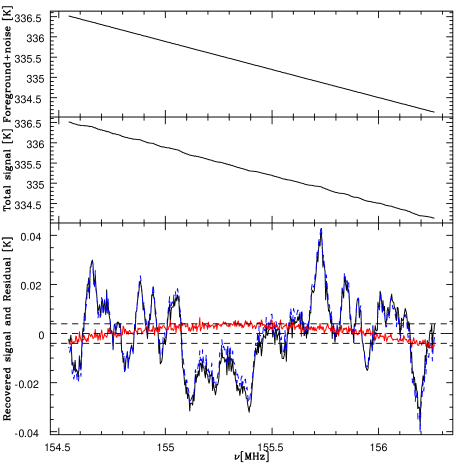
Figure 3.— Spectrum in a single pixel before and after foreground cleaning. The top panel shows total contaminant signal, consisting of synchrotron radiation ($A_{syn}=335.4{\rm K}$, $\alpha_{syn}=2.8$, $\Delta\alpha_{syn}=0.1$), free-free emission foreground ($A_{ff}=33.5{\rm K}$, $\alpha_{ff}=2.15$, $\Delta\alpha_{ff}=0.01$), extragalactic point sources ($\sigma_{\alpha}=10$) and detector noise ($\sigma=1{\rm mK}$). The middle panel has the cosmological 21cm signal added. The bottom panel shows the recovered 21cm signal (blue curve) compared with the true simulated signal (black curve) and the residual (recovered minus simulated 21cm signal; red curve). The three horizontal black dashed lines correspond to -0.004K, 0K, and 0.004K, respectively. (Note the different vertical axis limits.) The small-scale wiggles in the residual are detector noise, whereas the smoothed parabola-shaped component of the residual is the error in the foreground fitting.

By transforming the detector noise and the residual from the bottom panel of 3 back to $k$-space, we are able to compare them with the 21cm 1D power spectrum, shown in 4. Before foreground cleaning, the total contaminant (blue dotted curve) is seen to dominate over the 21cm power spectrum (black solid curve). The foreground power spectrum is seen to rise towards the left, reflecting its rather smooth frequency dependence. After foreground cleaning, the residual contaminant (red dashed curve) is significantly below both the original contaminant except on scales $k\ll 0.1h/$Mpc. The flat section of the residual power spectrum for $k\mathrel{\hbox to0.0pt{\lower 3.0pt\hbox{$\mathchar 536\relax$}\hss}\raise 2.0pt\hbox{$\mathchar 318\relax$}}1h/$Mpc is seen to correspond to detector noise.

The three vertical lines in 4 correspond to different minimum channel width for different upcoming experiments. From left to right, they are 0.1MHz (fiducial), 8kHz (for MWA) and 4kHz (for LOFAR). Information to the right of this minimum channel width line is lost, roughly corresponding an exponential blow-up of the effective detector noise. In other words, the effective detector noise goes much higher above the signal to the right of those lines so that little information can be extracted there. So in order to take advantage of our method of foreground removal, the channel width needs to be small enough to reach the noise-dominated region.

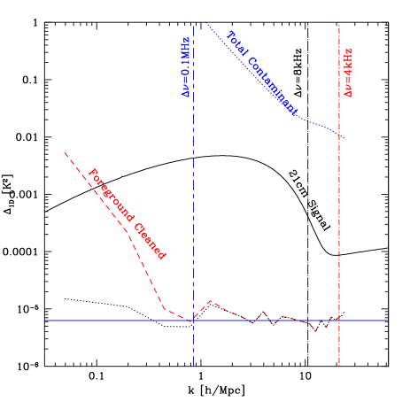
Figure 4.— 1D power spectra of 21cm signal (solid black curve), total contaminant from 3 (dotted blue curve), residual contaminant after foreground cleaning (dashed red curve) and detector noise alone (dotted black curve). The horizontal solid blue line is the white noise power spectrum used for the detector noise simulation. The three vertical lines correspond to the different channel width for different experiments. From left to right, they are 0.1MHz (fiducial, short dash - long dash blue line), 8kHz (for MWA, dot - long dash black line), and 4kHz (for LOFAR dot - short dash red line).

In other words, 21 cm tomography is limited mainly by foregrounds for $k\ll 1h/$Mpc and limited mainly by noise for $k\gg 1h/$Mpc. To take full advantage of their sensitivity by pushing residual foregrounds down to the detector noise levels, experiments should therefore be designed to have a channel width substantially smaller than 0.1 MHz. Such small channel widths are realistic and achievable for upcoming experiments. Since the analysis can now practically be done by dedicated high speed electronics, even if the software solution was not fast enough.

To test the robustness of our foreground cleaning technique, we repeated the above analysis for a wide range of foreground models with the same noise level.

First we tested a suite of models with only detector noise and synchrotron radiation, changing the values of the parameters defined in equation (10). Most of the results were similar to those shown in 3. Increasing the synchrotron amplitude parameter $A_{syn}$ all the way up to completely unrealistic value $10^{7}{\rm K}$ had essentially no effect, because in this case the simulated spectrum had the exact same shape as the model fit for in the cleaning step. Likewise, changing the spectral index $\alpha_{syn}$ over the extreme range $-80<\alpha_{syn}<20$ had little effect. Complicating the synchrotron spectrum with a running of the running term $\Delta\alpha_{syn}^{rr}\lg^{2}({\nu\over\nu_{*}})$, so that the intensity of the synchrotron foreground can be written as

$$I_{syn}=A_{syn}\left(\nu\over{\nu_{*}}\right)^{-\alpha_{syn}-\Delta\alpha_{syn}\lg{{\nu}\over{\nu_{*}}}-\Delta\alpha_{syn}^{rr}\lg^{2}({\nu\over\nu_{*}})},$$ (20)

still caused a negligible increase of the residual as long as $|\Delta\alpha_{syn}^{rr}|\leq 50$. This is a reflection of the fact that over a fairly narrow frequency range, even a more complicated function can be accurately approximated by a parabola in log-log, i.e., by the first three terms of its Taylor expansion.

Making variations around the baseline case of multiple foregrounds, similarly we tried numerous examples with either higher foreground amplitudes, different spectral indices or larger running of the spectral indices, again obtaining results similar to the ones shown in 3. For example, for the point source foreground, we tried different values for parameter $\sigma_{\alpha}$ in equation (13) from $\sigma_{\alpha}=0.2$ up to $\sigma_{\alpha}=100$. We found that as long as $\sigma_{\alpha}\leq 60$ (a conservative cut), the residuals are rather insensitive to the distribution of point source spectral indices.

All our tests show that as with astrophysically plausible foreground amplitudes, the effectiveness of our simple “blind” cleaning method is almost independent of the number, shape and amplitude of relatively smooth foregrounds.

The basic reason for this robustness is easy to understand. As long as the total foreground signal can be well-approximated by our fitting function (a log-log parabola) over the small frequency interval in question, then the main contribution to the residual will not be the foregrounds, but the amplitude of this log-log parabola contributed by random detector noise. Our numerical examples show that the residual indeed does have roughly the shape of our fitting function, not the shape of the main leading order contribution from residual foregrounds (the next term in their Taylor expansion, i.e., a cubic term).

4.2. Baseline example 2 — near term situation (noise$\gg$signal)

The detector white noise we assumed in previous example is small comparing to the signal, in which case we can subtract the foreground easily for each pixel. Nevertheless, that level of noise might not be achieved until future next generation experiments. For upcoming experiments, as we showed in equation (17) and equation (18), the detector noise is far above the 21cm signal.

In this section, we study the close term case by assuming detector noise $\sigma=200{\rm mK}$, 200 times larger than previous example, using the same baseline foreground model as in previous section.

One would expect that for each individual pixel, the huge white noise destroys much of the information about the 21 cm signal and also obscures the frequency dependence of the foregrounds, makeing them harder to fit and remove, and that the residual will be noise-dominated. In this scenario, single pixel cleaning is not enough for cleaning purposes and multiple pixels are needed to average down the noise and fit the foregrounds. However, complications arise when processing multiple pixels. Different pixels come from different lines of sight, so their 21cm signals are either slightly different realizations or completely independent realizations of equation (7), depending on how far apart the pixels are from one another. Furthermore, for pixels that are close to one another, they have slightly different signals in general, but on large scales, the signals within these pixels are more or less identical, while on small scales, the signals are almost independent of signals in other pixels. The detailes of this complication would probably best be treated via a detailed 3D numerical simulation, where thousands of pixels can be simulated and the signals from them tested. Since this is beyond the scope of this paper, we will simply illustrate the basic effects by two extreme situations, which can also be applied to numerically generated signals. We will see from the following examples that our method for foreground cleaning still works reasonably well.

4.2.1 Coherent signal approximation

For closely separated pixels, we make the crude assumption that the line of sight 21cm signal in these pixels are identical (same phase and amplitude as in equation (7)). This approximation will simplify our calculation, yet the procedure of doing foreground removal is similar to generally incoherent signals as we discuss in the next subsection.

Since the signals are coherent, the total signal for different pixels is the summation of the same signal and different foregrounds and noise. We use the same method as described in Subsection 4.1 to remove the foreground from total signal along line of sight for each individual pixel. We then average all of them in real space and obtain the averaged cleaned signal.

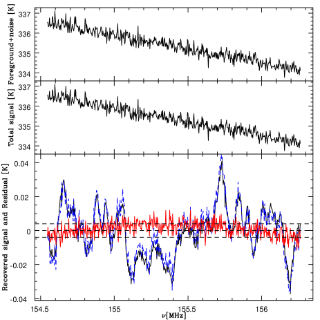
Figure 5.— Same as 3, but with 200 times larger detector noise ($\sigma=200{\rm mK}$). In the bottom panel, the recovered 21cm signal (blue curve) and the residual (red curve) is the result of averaging 4000 pixels. All other curves in the plot are from a single pixel.

Figure 5 shows the results before and after cleaning. The top and middle panels are plotted for a single pixel with 200mK noise. The noise wiggles fast on top of the foreground and dominates the signal. It is impossible to tell the difference between situations with and without 21cm signal (top and middle panels). The bottom panel shows the cleaned signal and residual by applying our method and combining 4000 such pixels. Although both foregrounds and noise are at a level orders of magnitude higher than the signal, the resulting cleaned signal still captures the main features of the “true” signal and the residual is well controlled.

This confirms that the foregrounds can still be removed effectively when the noise is orders of magnitude higher than the signal. Our fitting method does not introduce additional contamination to the signal, even when foregrounds with many different spectral shapes are averaged together.

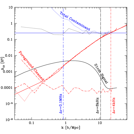
Figure 6.— Same as 4, but with 200 times larger detector noise ($\sigma=200{\rm mK}$). The coherent case residual contaminants (dot-dashed red curve) are FFT from coherently averaged residual in 5 (red curve). The incoherent case residual contaminant (red solid, dashed, and dotted curves) are computed from incoherently averaging 40000 pixels. The red solid, dashed, and dotted curves are assuming 1.7MHz, 8.6MHz, and 17.2MHz bandwidth, respectively.

Figure 6 shows $k$-space signal power spectrum compared with foregrounds and noise power spectra for single pixel and residual power spectrum from averaging 4000 pixels. Before cleaning, for each individual pixel, the signal is completely buried under huge noise and foregrounds. After cleaning, the residual (red dot-dashed curve) is orders of magnitude below both signal and original contaminants except on very large scales. Similar to 4, the plot suggests that we need frequency resolution substantially smaller than 0.1MHz to take advantage of foreground removal sensitivity.

The number of pixels needed to average down the noise varies sharply with the actual noise level. To achieve a similar level of accuracy shown in 5, for noise $\sim 500{\rm mK}$, we need approximately 20000 to 30000 pixels. For noise $\sim 100{\rm mK}$, we need around 1000 pixels. If the noise is about the same level as the signal $\sigma=20{\rm mK}$, we only need 50 to 100 pixels to adequately lower the noise.

When larger numbers of pixels getting combined, several side effects appear such as the variation of spectral indices among different pixels, signal and foreground angular correlation, overestimation of the sensitivity at small scales, etc. We will discuss some of these issues a bit more in the next subsection. The best approach, however, is to combine this method with angular approach and remove the contaminants in 3D (McQuinn et al., 2005; Morales, Bowman, & Hewitt, 2005). Although this is beyond the scope of the present paper, we hope to address this further in future work.

4.2.2 Incoherent signals

For pixels that are far apart, the line of sight 21cm signal in these pixels are no longer the same. They have different phases and amplitudes and therefore are more or less independent to one another. Here we study the case when all signals are completely independent. Compared to the case studied in the previous subsection, this case is the opposite extreme. Signals obtained from real observations will probably have a behavior intermediate between these tow extremes. Simulating such signals numerically, our cleaning technique is likely to give residual contaminant levels that are intermediate between those we find here for these two extreme cases.

When the signals are incoherent, we still use the same method to remove foregrounds from the total signal for each individual pixel. However, instead of averaging them in real space, we FFT the signal in each pixel to Fourier space to obtained the cleaned power spectrum for each pixel. Then we average all individual power from different pixels and get the final average cleaned power spectrum.

Comparing with averaging coherent signals in real space, averaging incoherent signals in Fourier space requires larger numbers of pixels to remove the foregrounds effectively. Figure 6 shows true 21cm power spectrum compared with residual foregrounds and noise power spectra (red solid, dashed, and dotted curves), defined as the difference between average cleaned power spectrum and true 21cm power spectrum, from incoherently averaging 40000 pixels. The noise and foregrounds levels are kept the same as in previous coherent example. Although we average 10 times more pixels here than for coherent case, the residual contaminant is at a level higher than the previous case. However, the residual is still reasonable. On most of the scales, the residual contaminant is less than 10% of the signal. Also notice in this case the 21cm power spectrum is best measured for scales around $k=0.1h/{\rm Mpc}$, another consequence from incoherence averaging. In previous two examples, namely low noise and high noise coherence signal examples, we recovered signal instead of power spectrum.

The three different residual curves in the plot are computed assuming 1.7MHz (red solid curve), 8.6MHz (red dashed curve), and 17.2MHz (red dotted curve) bandwidth, respectively. (We used 1.7MHz bandwidth for all previous calculations and figures.) As the bandwidth increases, the residual power decreased especially on smaller $k$. That is to say a larger bandwidth will help foreground removal at large scales.

So the bottom line is, for incoherent signals, our method for foreground cleaning still works, yet its efficiency is reduced due to the fact that signals are independent. In this case, we could consider increase bandwidth, combine with angular direction measurements, etc., to improve efficiency and remove foregrounds effectively.

5. Discussion

We have explored how well foreground contamination can be removed from a 21 cm tomography data cube by using frequency dependence alone. We found that with realistic experimental sensitivities, 21 cm tomography is limited mainly by foregrounds for scales $k\ll 1h/$Mpc and limited mainly by noise for $k\gg 1h/$Mpc, a result which is rather robust to changing the foreground assumptions. In optimizing the design of upcoming experiments, a useful rule of thumb is therefore to make the channel width substantially smaller than 0.1 MHz, allowing one to take full advantage of the detector sensitivity by pushing residual foregrounds down to the noise level. Fortunately, attaining such narrow channel width is realistic for upcoming experiments, where the analysis is all done in dedicated high speed electronics.

We used a simple “blind” removal technique using no prior information about the nature of the foregrounds, merely fitting out a quadratic polynomial in log-log for the frequency dependence separately for each pixel in the sky. The basic reason that this works so well is that the foregrounds have a much smoother frequency spectra than the 21 signal.

Although highly effective, this frequency-based cleaning should be viewed as merely one of three complementary foreground countermeasures. First, bright point sources can be identified as strong positive outliers, and the corresponding sky pixels can be discarded since they constitute only a small fraction of the total survey area. Second, after the frequency-based cleaning step, noise and signal can be further distinguished by their different angular correlations, as described in Santos et al. (Santos, Cooray, & Knox, 2004). This angular approach will be particularly helpful for early 21 cm experiments where the signal-to-noise ratio is limited. The angular and frequency-based approaches are therefore complementary, and the combination of the two will give the best cleaned 21cm signal with which to study the “dark” epoch of reionization.

Although our results are quite encouraging for the prospects of doing cosmology with 21 cm tomography, much work remains to be done on the foreground problem, and we conclude by mentioning a few examples.

A key assumption is this paper is that the foregrounds are dominated by emission mechanisms producing fairly smooth spectra. The basis for this assumption is that typical atomic and molecular transitions that can produce spectral lines correspond to much higher frequencies than those relevant to 21 cm tomography. One loophole that needs to checked quantitatively is the possible contribution of recombination lines from hydrogen cascading down though very large energy quantum numbers $n\sim 10^{7}$, although early estimates suggest that this is not a significant contaminant (e.g., Oh & Mack, 2003).

We performed our analysis on simulated data over a small redshift range, limited by our linearization approximation. It is clearly worthwhile repeating our analysis with a proper hydrodynamical simulation of the 21 cm signal over the full relevant redshift range. In this case, our 3-parameter foreground fit should be generalized to one that assumes that the foregrounds are simple only locally in log-frequency space. An obvious generalization of our method would be to increase the order of the log-log polynomial beyond two. However, we effectively want to high-pass filter the observed frequency spectrum to clean out foregrounds, and high-order polynominals can in principle spoil this by having sharp localized features. A better generalization of our method to long frequency baselines may therefore be either a cubic spline in log-log or a Fourier series expansion. Such end-to-end simulations will also be a valuable tool for quantifying how redshift space distortions (whereby the peculiar velocity of the gas breaks the one-to-one correspondence between redshift and frequency) can be exploited to separate the effects of the matter power spectrum from the “gastrophysics” (Barkana & Loeb, 2004b). This becomes important especially for channel width $\mathrel{\hbox to0.0pt{\lower 3.0pt\hbox{$\mathchar 536\relax$}\hss}\raise 2.0pt\hbox{$\mathchar 316\relax$}}0.1{\rm MHz}$ (Desjacques & Nusser, 2004; Iliev et al., 2002b).

In summary, the potential science return from 21 cm tomography is enormous, both for understanding the reionization epoch and for probing inflation and dark matter with precision measurements of the small-scale power spectrum. Our calculations strengthen the conclusion that foreground contamination will not be a show-stopper. The current situation is similar to the quest for the cosmic microwave background in the 1980’s in that the cosmological signal has not yet been detected, but better in the sense that the amplitude of both signals and foregrounds are approximately known, guaranteeing success if the engineering challenges can be overcome.

References

- (1)
- Barkana & Loeb (2004a) Barkana, R. and Loeb, A. 2005, ApJ, 626, 1
- Barkana & Loeb (2004b) Barkana, R. and Loeb, A. 2005, ApJ, 624, L65
- Becker et al. (2001) Becker, R. H. et al. 2001, AJ, 122, 2850
- Bennett et al. (2003) Bennett, C. et al. 2003, ApJ, 148, 97
- Bowman et al. (2005) Bowman, J. D., Morales, M. F., and Hewitt, J. N. 2005, astro-ph/0512262
- Carilli et al. (2004b) Carilli, C., Furlanetto, S., Briggs, F., Jarvis, M., Rawlings, S., and Falcke, H. 2004, New Astron Rev, 48, 1029
- Carilli et al. (2004a) Carilli, C. L., Gnedin, N., Furlanetto, S., and Owen, F. 2004, New Astron. Rev., 48, 1053
- Carilli, Gnedin, & Owen (2002) Carilli, C., Gnedin, N. Y., and Owen, F. 2002, ApJ, 577, 22
- Ciardi & Madau (2003) Ciardi, B. and Madau, P. 2003, ApJ, 596, 1
- Desjacques & Nusser (2004) Desjacques, V. and Nusser, A. 2004, MNRAS, 351, 1395
- Dimatteo, Ciardi, & Miniati (2004) Di Matteo, T., Ciardi, B., and Miniati, F. 2004, MNRAS, 355, 1053
- DiMatteo et al. (2002) Di Matteo, T., Perna, R., Abel, T., and Rees, M. J. 2002, ApJ, 564, 576
- Fan et al. (2002) Fan, X. et al. 2002, AJ, 123, 1247
- Field (1958) Field, G. B. 1958, Proc. IRE, 46, 240
- Field (1959) Field, G. B. 1959, ApJ, 129, 551
- Furlanetto & Briggs (2004) Furlanetto, S. and Briggs, F. 2004, New Astron. Rev., 48, 1039
- Furlanetto, Sokasian, & Hernquist (2004) Furlanetto, S. R., Sokasian, A., and Hernquist, L. 2004, MNRAS, 347, 187
- Furlanetto, Zaldarriaga, & Hernquist (2004) Furlanetto, S., Zaldarriaga, M., and Hernquist, L. 2004, ApJ, 613, 16
- Gnedin & Shaver (2003) Gnedin, N. Y. and Shaver, P. A. 2004, ApJ, 608, 611
- Gunn & Peterson (1965) Gunn, J. E. and Peterson, B. A. 1965, ApJ, 142, 1633
- Haiman & Holder (2003) Haiman, Z. and Holder, G. P. 2003, ApJ, 595, 1
- Haslam et al. (1982) Haslam, C. G. T., Stoffel, H., Salter, C. J., and Wilson, W. E. 1982, A&AS, 47, 1
- Haverkorn, Katgert, & de Bruyn (2003) Haverkorn, M., Katgert, P., and de Bruyn, G. 2003, A&A, 403, 1031
- Hewitt (2004) Hewitt, J. N., private communications.
- Holder et al. (2003) Holder, G., Haiman, Z., Kaplinghat, M., and Knox, L. 2003, ApJ, 595, 13
- Hui, Stebbins, & Burles (1999) Hui, L., Stebbins, A., and Burles, S. 1999, ApJ, 511, L5
- Iliev et al. (2002a) Iliev, I. T., Shapiro, P. R., Ferrara, A., and Martel, H. 2002, ApJ, 572, L123
- Iliev et al. (2002b) Iliev, I. T., Scannapieco, E., Martel, H., and Shapiro, P. R. 2003, MNRAS, 341, 81
- Knox (2003) Knox, L. 2003, New Astron. Rev., 47, 883
- Kogut et al. (2003) Kogut, A. et al. 2003, ApJS, 148, 161
- Liddle & Lyth (2000) Liddle, A. R. and Lyth, D. H. 2000, Cosmological Inflation and Large-Scale Structure (Cambridge Univ. Press: Cambridge)
- Loeb & Zaldarriaga (2004) Loeb, A. and Zaldarriaga, M. 2004, PRL, 92, 211301
- Madau, Meiksin, & Rees (1997) Madau, P., Meiksin, A., and Rees, M. J. 1997, ApJ, 475, 492
- McQuinn et al. (2005) McQuinn, M., Zahn, O., Zaldarriaga, M., Hernquist, L., and Furlanetto, S. R. 2005, astro-ph/0512263
- Morales (2004) Morales, M. F. 2005, ApJ, 619, 678
- Morales, Bowman, & Hewitt (2005) Morales, M. F., Bowman, J. D., and Hewitt, J. 2.005, astro-ph/0510027
- Morales & Hewitt (2003) Morales, M. F. and Hewitt, J. 2004, ApJ, 615, 7
- Oh & Mack (2003) Oh, S. P. and Mack, K. J. 2003, MNRAS, 346, 871
- Peacock (1999) Peacock, J. A. 1999, Cosmological Physics (Cambridge Univ. Press: Cambridge)
- Pen, Wu, & Peterson (2004) Pen, U-L., Wu, X-P., and Peterson, J. 2004, astro-ph/0404083
- Platania et al. (2003) Platania, P., Burigana, C., Maino, D., Caserini, E., Bersanelli, M., Cappellini, B., and Mennella, A. 2003, A&A, 410, 847
- Purcell & Field (1956) Purcell, E. M. and Field, G. B. 1956, ApJ, 124, 542
- Rottgering (2003) Rottgering, H. et al. 2003, TSRA Symp., , 69
- Santos et al. (2003) Santos, M. G., Cooray, A., Haiman, Z., Knox, L. , and Ma, C-P. 2003, ApJ, 598, 756
- Santos, Cooray, & Knox (2004) Santos, M. G., Cooray, A., and Knox, L. 2005, ApJ, 625, 575
- Seljak et al. (2004) Seljak, et al.. 2005, Phys. Rev. D, 71, 103515
- Shaver et al. (1999) Shaver, P. A., Windhorst, R. A., Madau, P., and de Bruyn, A. G. 1999, A&A, 345, 380
- Spergel et al. (2003) Spergel, D. N. et al. 2003, ApJS, 148, 175
- Spergel et al. (2006) Spergel, D. N. et al. 2006, astro-ph/0603449
- Tegmark (1997) Tegmark, M. 1997, ApJ, 480, L87
- Tegmark (1998) Tegmark, M. 1998, ApJ, 502, 1
- Tegmark et al. (2000) Tegmark, M., Eisenstein, D. J., Hu, W., and de Oliveira-Costa, A. 2000, ApJ, 530, 133
- Tegmark & de Oliveira-Costa (1998) Tegmark, M. and de Oliveira-Costa, A. 1998, ApJ, 500, L83
- Tegmark, de Oliveira-Costa, & Hamilton (2003) Tegmark, M., de Oliveira-Costa, A., and Hamilton, A. 2003, Phys. Rev. D, 68, 123523
- Tegmark et al. (2004) Tegmark, M. et al. 2004, Phys. Rev. D, 69, 103501
- Tozzi et al. (2000) Tozzi, P., Madau, P., Meiksin, A., and Rees, M. J. 2000, ApJ, 528, 597
- Wouth (1952) Wouthuysen, S. A. 1952, AJ, 57, 31
- Wyithe & Loeb (2004a) Wyithe, S. and Loeb, A. 2004, ApJ, 610, 117
- Wyithe & Loeb (2004b) Wyithe, S. and Loeb, A. 2004, Nature, 432, 194
- Zaldarriaga, Furlanetto, & Hernquist (2003) Zaldarriaga, M., Furlanetto, S. R., and Hernquist, L. 2004, ApJ, 608, 622