The Spitzer Space Telescope First-Look Survey:
Neutral Hydrogen Emission

Abstract

The Spitzer Space Telescope (formerly SIRTF) extragalactic First-Look Survey covered about 5 deg² centered on J2000 $\alpha=17^{\rm h}18^{\rm m}$, $\delta=59^{\circ}30^{\prime}$ in order to characterize the infrared sky with high sensitivity. We used the 100-m Green Bank Telescope to image the 21 cm Galactic H I emission over a $3\arcdeg\times 3\arcdeg$ square covering this position with an effective angular resolution of $9\farcm 8$ and a velocity resolution of 0.62 km s^-1. In the central square degree of the image the average column density is $N_{\rm HI}=2.5\times 10^{20}$ cm^-2 with an rms fluctuation of $0.3\times 10^{20}$ cm^-2. The Galactic H I in this region has a very interesting structure. There is a high-velocity cloud, several intermediate-velocity clouds (one of which is probably part of the Draco nebula), and narrow-line low velocity filaments. The H I emission shows a strong and detailed correlation with dust. Except for the high-velocity cloud, all features in the $N_{\rm HI}$ map have counterparts in an $E(B-V)$ map derived from infrared data. Relatively high $E(B-V)/N_{\rm HI}$ ratios in some directions suggest the presence of molecular gas. The best diagnostic of such regions is the peak H I line brightness temperature, not the total $N_{\rm HI}$: directions where $T_{\rm b}>12$ K have $E(B-V)/N_{\rm HI}$ significantly above the average value. The data corrected for stray radiation have been released via the Web.

1 Introduction

The Space Infrared Telescope Facility (SIRTF) was launched in 2003 and renamed the Spitzer Space Telescope. Following the in-orbit checkout, it began the First-Look Survey (FLS) of selected areas to characterize the far-infrared (FIR) sky two orders of magnitude deeper than was reached by previous instruments (see http://ssc.spitzer.caltech.edu/fls/). The extragalactic portion of the FLS covers about $5\,{\rm deg^{2}}$ centered on J2000 $\alpha=17^{\rm h}18^{\rm m}$, $\delta=+59^{\circ}30^{\prime}$. Most of the extragalactic FIR sources are expected to have radio continuum counterparts obeying the FIR/radio correlation, so this region has been imaged by the VLA with matching sensitivity at 1.4 GHz (Condon et al., 2003). Because there is a good correlation between Galactic FIR emission and the column density of H I at high Galactic latitudes (Boulanger & Perault, 1988; Boulanger et al., 1996; Schlegel, Finkbeiner, & Davis, 1998; Hauser, 2001), high-quality 21cm H I data from this region can be used to estimate foreground Galactic cirrus emission which might confuse extragalactic studies. The H I data are also useful for studying properties of Galactic dust seen in the FIR (e.g., Boulanger et al. 2001).

We have observed the area of the FLS survey in the 21 cm line of H I with the Green Bank Telescope (GBT). The data give accurate values of the neutral hydrogen column density $N_{\rm HI}$ throughout the field and reveal interesting interstellar structures, most of which are visible in existing FIR data.

2 Observations and Data Reduction

We used the Robert C. Byrd Green Bank Telescope (GBT) (Lockman, 1998; Jewell, 2000) to measure the 21 cm H I emission over the FLS field six times during three observing sessions in 2002, 2003, and 2004. The GBT has a half-power beam width of $9\farcm 2$ in the 21 cm line at 1.420 GHz. The total system temperature toward the FLS field was $\leq 20$ K, and the receiver recorded both circular polarizations. For this experiment the telescope was scanned in right ascension at a constant declination, then the declination was stepped by $3^{\prime}$ and the scan direction was reversed. The resulting images cover an area of $3\arcdeg\times 3\arcdeg$ in right ascension and declination centered on J2000 $\alpha=17^{\rm h}18^{\rm m}$, $\delta=+59\arcdeg 30\arcmin$ ($\ell=88\fdg 32$, $b=+34\fdg 89$). Within this area H I spectra were measured every 3′ in both coordinates. The integration time was 3 s per pixel for each of the six maps, and data were taken by frequency switching out of the band. The spectra cover about 520 km s^-1 centered at $V_{\rm LSR}=-50$ km s^-1 with a channel spacing of 0.52 km  s^-1 and an effective velocity resolution of 0.62 km s^-1.

The spectral brightness temperature scale was determined from laboratory measurements of the noise diode and checked with frequent observations of the standard regions S6 and S8 (Williams, 1973; Kalberla, Mebold, & Reif, 1982). We used aips++ to regrid and average the spectra into a single data cube with a pixel size of $1\farcm 5$. Third-degree polynomials were fit to line-free regions of the spectra and subtracted, and a correction for stray radiation was applied as described below, yielding a final data cube with the properties given in Table 1. The regridding broadened the effective angular resolution to a FWHM of $9\farcm 8$.

2.1 Stray Radiation

Ideally, all signals received by a radio telescope would come through the main antenna beam. Real telescopes, however, always have sidelobes. These sidelobes cause special problems for observations of Galactic H I because there is Galactic 21 cm H I emission from every direction on the sky. All telescope sidelobes not falling on the ground thus contribute “stray” radiation which must be subtracted if accurate H I spectra are to be obtained. Unlike all other large antennas, the GBT has an unblocked optical path and should have a minimum of stray H I radiation. However, the feed horn currently used for 21 cm observations is part of a general purpose L-band system covering 1.15 GHz – 1.73 GHz from the Gregorian focus. Because of structural limitations on its size and weight, this feed over-illuminates the 8 m diameter secondary reflector at the 1.420 GHz frequency of the 21 cm line, creating a broad and diffuse forward spillover lobe which contains about 4% of the telescope’s response (Norrod & Srikanth 1996; S. Srikanth, private communication). Efforts are underway to model and measure this sidelobe. Its importance for observations of the FLS field is illustrated by Figure 1, which shows the striking difference between two GBT H I spectra of the same sky area observed at different local sidereal times (LSTs). The differences between the spectra are due entirely to changes in the stray radiation. In Figure 2, the the two ovals show the GBT subreflector in Galactic coordinates as seen from the focal point at the times the two observations were made. When the upper rim of the subreflector lies at low latitude, e.g., at 23^h LST, the spillover lobe picks up the very bright H I emission from the Galactic plane, whereas at 10^h LST the subreflector rim lies primarily on faint H I at high Galactic latitude. The general characteristics of the profiles in Figure 1 suggest that this understanding of the origin of the difference between the spectra is correct.

The best way to compensate for stray radiation entering a telescope’s sidelobes is to determine the telescope’s response in all directions, estimate the contribution from H I in directions away from the main beam, and subtract that from the observed spectra. This method has been used successfully to correct data from several instruments (Kalberla, Mebold, & Reich, 1980; Hartmann et al., 1996; Higgs & Tapping, 2000), but it is quite laborious and requires knowledge of a telescope’s sidelobes in directions where they are very weak. Moreover, it is not certain that developing this technique for the GBT will be worth the effort because, unlike conventional reflectors whose sidelobes are caused by aperture blockage which can never be eliminated, the strongest sidelobes of the GBT are consequences of the specific feed and are not at all fundamental.

For the immediate purposes of this work, we estimated the stray component in the FLS field by “bootstrapping” the GBT data to the Leiden-Dwingeloo survey data in the general manner described by Lockman, Jahoda, & McCammon (1986) and Lockman (2003). This method assumes that the stray component of a 21 cm spectrum, which typically arises from broad sidelobes, does not change significantly with changes in main-beam pointing of a few degrees, and is also approximately constant during the few hours it takes to make one map. Each GBT map of the FLS field was made over 3 hours, so it is plausible that over this period the stray radiation spectrum can be approximated by a single average profile. That profile can be determined by convolving the GBT H I image to the angular resolution of the Leiden-Dwingeloo (hereafter LD) survey, which was made by a 25 m telescope having 36′ resolution (Hartmann & Burton, 1997) and was corrected for stray radiation using an all-sky model of its response (Hartmann et al., 1996). Any difference between the GBT data convolved to 36′ resolution, and the LD survey spectra at the same position, can be attributed to stray radiation in the GBT data.

We applied this technique to the GBT observations of the FLS. The GBT data were convolved to the 36′ resolution of the LD survey and compared with LD observations in the central area of the FLS field using a revised version of the LD survey with an improved stray-radiation correction kindly supplied by P. Kalberla. The difference spectra have the expected characteristics of stray radiation given the location of the GBT spillover lobe on the sky at the times of the observations. There are two exceptions, however: (1) the high-velocity cloud at $V_{\rm LSR}\approx-190$ km s^-1 and (2) the narrow, bright, spectral feature near $V_{\rm LSR}=0$ which appears in many directions over the FLS field. For both features the naive “bootstrapping” procedure gives inconsistent, implausibly large, and sometimes unphysically negative corrections to the GBT data. We believe that these problems are caused by limitations in the LD survey and its stray-radiation correction. The LD survey used its own data as the H I sky for determining stray-radiation corrections in an iterative procedure, but that H I sky was undersampled, being measured only every $0\fdg 5$. Thus real features near their main beam that have angular structure or velocity gradients on scales $\lesssim 0\fdg 5$ will be aliased into an erroneous stray-radiation correction. The potential for this sort of systematic effect was noted by the LD survey group (Hartmann et al., 1996), and we believe it occurs at velocities that have the greatest fractional variation in $T_{b}$ across the FLS field: those of the high-velocity cloud and those of the bright, low-velocity, narrow lines.

In the bootstrapping technique that we adopted after much experimentation, a GBT H I image was convolved with a circular Gaussian function to 36′ angular resolution and compared to LD survey spectra at eight locations near the field center. Because stray radiation is expected to be significant only at velocities $|V_{\rm LSR}|\lesssim 100$ km s^-1, the observed GBT data were taken to be correct at $|V_{\rm LSR}|>125$ km s^-1. To compensate for the unphysical estimate of the stray radiation at the velocity of the narrow bright line, the stray spectrum was interpolated over the velocity range $-9\leq V_{\rm LSR}\leq+2.5$ km s^-1 which contains this feature. The stray column densities derived in this way vary from $0.1\times 10^{20}$ cm^-2 for the data taken at LST 10^h to $1.2\times 10^{20}$ cm^-2 for the data taken at 23^h. On the whole, the correction procedure appears to produce consistent results for all six images when they are processed separately, so we averaged them to produce the final data cube. Figure 3 shows the uncorrected 21 cm spectrum averaged over the central part of all the maps of the FLS, and the average spectrum of the stray radiation which was subtracted from it, which has an equivalent $N_{\rm HI}=4.9\times 10^{19}$ cm^-2.

Work is now underway on projects that we hope will eliminate the GBT’s forward spillover lobe at 21 cm, greatly improving its performance for H I observations, and making procedures like this unnecessary in the future. We note that the forward spillover lobe is important only at frequencies 1 – 2 GHz. Over most of its frequency range the GBT has an exceptionally clean antenna pattern.

2.2 Error Estimates

For $|V_{\rm LSR}|>125$ km s^-1 uncertainties in the final spectra are dominated by random noise, while for velocities closer to zero the uncertainties arise mainly from the correction for stray radiation. An estimate of the latter was derived by comparing data cubes that had quite different amounts of stray radiation removed. The comparison suggests that our correction for stray radiation may introduce an rms error of 0.1 K for $|V_{LSR}|\gtrsim 30$ km s^-1, and as much as 0.25 K for the brighter emission near zero velocity. At the eight positions across the final image where the stray correction was derived, the integrated correction has a standard deviation equivalent to $N_{\rm HI}=1.0\times 10^{19}$ cm^-2, which should be a reasonable estimate for this error term. We checked for temporal variations in the stray correction by looking for systematic offsets in corrected spectra as a function of time, but found nothing significant. The rms instrumental noise $\sigma\approx 0.08$ K was derived from fluctuations in emission-free channels and is in good agreement with theoretical estimates. Table 2 summarizes these uncertainties.

2.3 Creation of the $N_{\rm HI}$ Data Cubes

After correction for stray radiation, the spectra were converted from units of brightness temperature $T_{\rm b}(V)$ to H I column density per channel $N_{\rm HI}(V)$. This step requires knowledge of the excitation temperature (called the spin temperature $T_{\rm s}$) of the 21 cm transition, which usually cannot be determined from the 21 cm emission spectra themselves (Dickey & Lockman, 1990; Liszt, 2001; Lockman, 2004). Two conversions were therefore made: one assuming $T_{\rm s}=10^{4}$ K, which corresponds to optically thin emission, and the other for $T_{\rm s}=80$ K, a value appropriate for diffuse clouds (Savage et al., 1977) and one which is more realistic for the narrow line at low velocity which must arise from gas with $T_{\rm s}\leq 160$ K ($\S 3.1$). Most of the H I emission has a $T_{\rm b}(V)$ of only a few Kelvins, so the difference in assumed $T_{\rm s}$ affects the total $N_{\rm HI}$ by only a few percent. However, at the velocities of the brightest lines, e.g., around $V_{\rm LSR}=-2$ km s^-1, $N_{\rm HI}(T_{s}=80)/N_{\rm HI}(thin)$ can be as large as 1.2. In all likelihood, $T_{\rm s}$ varies across every 21cm H I spectrum (Liszt, 1983). Uncertainty in the conversion of $T_{b}$ to $N_{\rm HI}$ affects the interpretation of dust-to-gas ratios in parts of the FLS field (§4). The fundamental data cube of $T_{\rm b}(\alpha,\delta,V)$ is available for anyone who wishes to make a different conversion to $N_{\rm HI}(V)$.

The final data product is three cubes, available via http://www.cv.nrao.edu/fls$\_$gbt in FITS format. Data at the extreme ranges of velocity which contain no emission have been omitted from the final cubes. The data before correction for stray radiation are also available from F. J. Lockman upon request.

3 H I in the FLS Field

3.1 Selected H I Features

H I spectra from the FLS field (e.g., Fig. 3) typically contain four components: (1) a broad line near zero velocity which contains most of the emission in most directions, (2) a bright, narrow line also near zero velocity which has a patchy though spatially correlated structure, (3) several clouds at intermediate negative velocities, and (4) a high-velocity cloud.

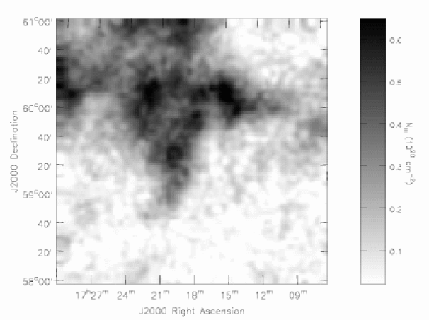
Figure 4: H I in the FLS field integrated over $-230\leq V_{\rm LSR}\leq-130$ km s^-1 showing emission arising from high-velocity cloud Complex C.

The high-velocity cloud appears over much of the FLS field, particularly at the higher declinations. It has a strong velocity gradient from $V_{\rm LSR}=-190$ km s^-1 in the east, where it is brightest, to $V_{\rm LSR}=-155$ km s^-1 in the west. This is part of high-velocity Complex C, a large sheet of gas which extends $>100^{\circ}$ across the sky and is at least 5 kpc distant (Wakker & van Woerden, 1991). The H I column density integrated over the velocity of the cloud is shown in Figure 4. The peak $N_{\rm HI}$ of $6.9\times 10^{19}$ cm^-2 is about one-quarter of the total $N_{\rm HI}$ in that direction.

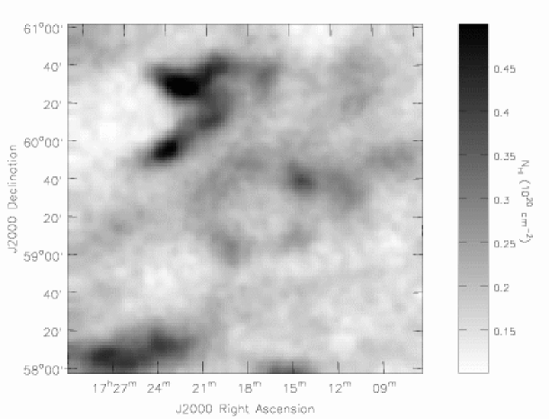
Figure 5: H I in the FLS field integrated over $-45\leq V_{\rm LSR}\leq-35$ km s^-1 showing several of the intermediate-velocity clouds.

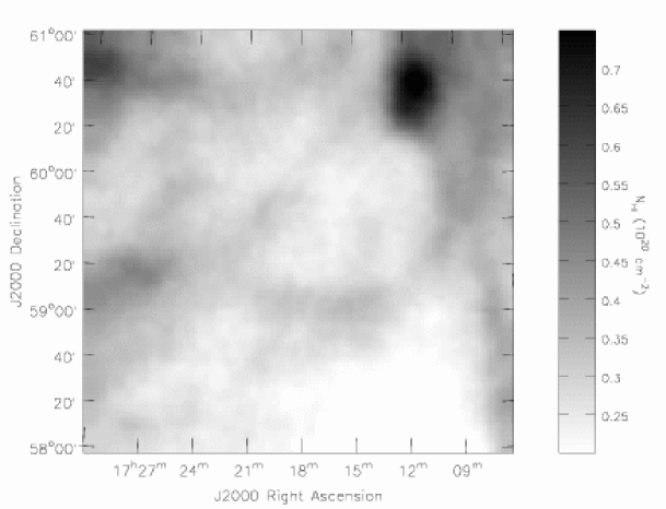
Figure 6: H I in the FLS field integrated over $-29\leq V_{\rm LSR}\leq-17$ km s^-1 highlighting emission from the small intermediate-velocity cloud at $\delta=60\arcdeg 41\arcmin$ associated with the Draco nebula.

Several H I clouds at an intermediate negative velocity are visible in the FLS field (Figs. 5 and 6). Properties of these clouds are listed in Table 3. Some are smaller than the GBT beam. They contribute 10% – 25% to the total $N_{\rm HI}$ in their directions. Unlike high-velocity clouds, which do not show FIR emission (Wakker & Boulanger, 1986), intermediate-velocity clouds are highly correlated with $I_{100\mu{\rm m}}$, though sometimes with a smaller $I_{100\mu{\rm m}}/N_{\rm HI}$ ratio than quiescent gas (Deul & Burton, 1990). Of special interest is the rather simple cloud shown in Figure 6, which seems to be part of the Draco nebula, an object $\gtrsim 600$ pc distant. The Draco nebula is quite distinct at $100\mu$m and is seen in absorption against the soft X-ray background (Burrows & Mendenhall, 1991; Herbstmeier et al., 1996; Gladders et al., 1998; Penprase, Rhodes, & Harris, 2000).

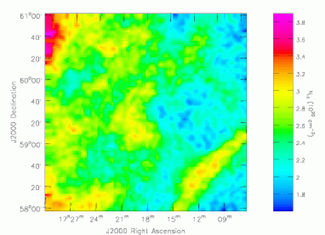
Figure 7: The $N_{\rm HI}$ over the FLS field integrated over all velocities after correction for stray radiation, evaluated for an assumed excitation temperature $T_{\rm s}=80$ K. The ‘arc’ discussed in the text is the feature to the lower right. It arises from a narrow, bright, low-velocity line.

Finally, the integrated $N_{\rm HI}$ image of Fig. 7 shows an arc of emission to the south-west (lower right) which arises in a narrow line at $V_{\rm LSR}=-2$ km s^-1. The line-width of 2.7 km s^-1 FWHM implies that the gas has a kinetic temperature $T\leq 160$ K. This is the brightest line in the field, reaching a peak $T_{\rm b}=26$ K, corresponding to $\tau_{HI}=0.4$ and $N_{\rm HI}=1.8\times 10^{20}$ cm^-2 for $T_{s}=80$ K. Most of the emission in the arc appears to be resolved by the beam of the GBT, though there may be small unresolved components.

3.2 Integral Properties

The H I column density for $T_{\rm s}=80$ K integrated over all velocities is shown in Figure 7. The visible structure is caused by specific interstellar objects, many of which have been discussed above. Table 4 lists values of $N_{\rm HI}$ averaged over various areas centered on the FLS central position. Over 9 deg² the total $N_{\rm HI}$ varies by only a factor of two, with an rms scatter 13% of the mean. As in most directions at high Galactic latitude, structure in H I over the FLS field is highly spatially correlated; significant fluctuations in total $N_{\rm HI}$ do not arise randomly or from tiny clouds (e.g., Schlegel, Finkbeiner, & Davis (1998); Miville-Deschen̂es et al. (2003); Lockman (2004)).

4 Infrared – H I Correlations

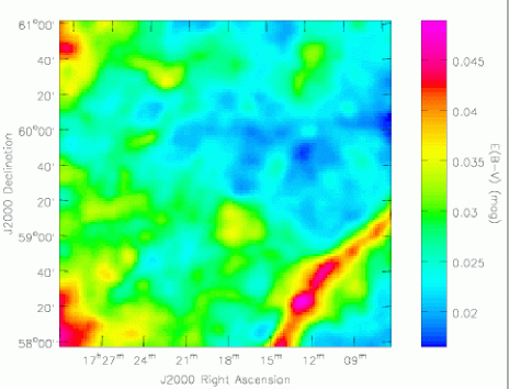
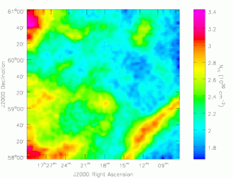
Figure 8: Top Panel: $E(B-V)$ over the FLS field derived by Schlegel, Finkbeiner, & Davis (1998) from temperature-corrected ${100\mu{\rm m}}$ data at $6\farcm 1$ angular resolution. Bottom Panel: Column density $N_{\rm HI}$ for $T_{\rm s}=80$ K from the GBT observations integrated over $V_{\rm LSR}>-100$ km s^-1 which excludes the high-velocity cloud. The bottom panel should be compared to Figure 7, which includes H I from the high-velocity cloud, to illustrate the absence of FIR emission from high-velocity clouds.

Schlegel, Finkbeiner, & Davis (1998) hereafter SFD, have derived the dust column density across the sky from temperature-corrected $100\mu$m data, and have expressed it as a reddening $E(B-V)$. Figure 8 shows their values of $E(B-V)$ over the FLS field at full resolution. (The SFD maps have an angular resolution of $6\farcm 1$, but quantitative comparisons with H I are made using the SFD maps smoothed to the angular resolution of the H I maps.) Most dust features have exact counterparts in H I. The correlation is shown explicitly in the left panel of Figure 9, where the FIR-derived reddening $E(B-V)$ is plotted against $N_{\rm HI}$.

The H I spectra consist of many components, and correlations performed between $E(B-V)$ and $N_{\rm HI}$ in various velocity intervals show that high-velocity Complex C must have a $100\mu$m emissivity per H I atom at least an order of magnitude smaller than the other H I components. For Complex C, the $3\sigma$ limit is $I_{100\mu\rm{m}}/N_{\rm HI}<5\times 10^{-22}$ MJy sr^-1 cm², while the ratio ranges between 50 and 70 in the same units for H I at other velocities in the FLS field, values comparable to those found in other studies (e.g., Heiles, Haffner, & Reynolds (1999); Lagache et al. (2000)). This confirms previous findings of only upper limits on $I_{100\mu{\rm m}}$ from high-velocity clouds (Wakker & Boulanger, 1986; Wakker & van Woerden, 1997). Complex C has low metallicity and contains little dust (Tripp et al., 2003) which can account for its low FIR emissivity. The right panel of Figure 9 shows the $E(B-V)$ vs. $N_{\rm HI}$ when H I associated with the high-velocity cloud is not included. The scatter is greatly reduced.

The lines in Fig. 9 are fit to $E(B-V)=a_{0}+a_{1}N_{\rm HI}(T_{s}=80$ K) and the coefficients $a_{0}$ and $a_{1}$ are listed in Table 5. The lower panel of Figure 8 shows $N_{\rm HI}$ for $T_{\rm s}=80$ K without the high-velocity cloud. In contrast to the H I map of Fig. 7, which includes all H I, this $N_{\rm HI}$ map appears nearly identical to the dust map, though there remain interesting anomalous regions. A map of the ratio $E(B-V)/N_{\rm HI}$ over the FLS field is shown in Figure 10. The ratio varies between 0.9 and 1.5 with a mean of $1.17\pm 0.09\times 10^{-22}$ mag cm².

4.1 Infrared – H I Variations

A detailed analysis of the gas and dust in the FLS field is beyond the scope of this paper, for there issues of dust properties and temperature, the conversion between $I_{100\mu\rm{m}}$ and $E(B-V)$, and the dust associated with ionized gas (Lagache et al., 1999, 2000). Here we will consider only what can be learned from the H I about possible sources of the variation in $E(B-V)/N_{\rm HI}$ across the FLS field, for some variations in the ratio seem tied to the properties of the 21cm line.

A significant aspect of Fig. 10 is that spatial structure in the dust-to-gas ratio is highly correlated, a fact that has been known for some time (e.g., SFD). Perhaps surprisingly, high dust-to-gas ratios come preferentially from areas of high $N_{\rm HI}$. One can see in the right panel of Fig. 9 that high $N_{\rm HI}$ directions are redder than a strict linear relationship would suggest. Table 5 includes results of a linear fit to only that data with $E(B-V)<0.03$, equivalent to $N_{\rm HI}\lesssim 2.5\times 10^{20}$ cm^-2; the slope is significantly flatter than when all reddenings are included. But higher reddening per unit $N_{\rm HI}$ does not simply track areas of high $N_{\rm HI}$: the greatest $N_{\rm HI}$ in the FLS field is in the upper left, yet it has an average value of $E(B-V)/N_{\rm HI}$ and is not at all conspicuous in Fig. 10. We find, instead, that the best predictor of a high $E(B-V)/N_{\rm HI}$ over the FLS field is the peak brightness temperature in the 21cm line, as shown in Figure 11. There seems to be excess reddening when spectra have a peak $T_{\rm b}\gtrsim 12$ K, and the discrepancy increases as the line gets brighter. The spectra with the highest $T_{b}$ are those toward the ‘arc’ at $V_{\rm LSR}\approx 0$. Similar, and possibly related line components cover much of the map. Assuming that the values of $E(B-V)$ are accurate, we consider three possibilities which might explain the increased reddening in this component.

First, the values of $N_{\rm HI}$ we derive would be underestimates if the gas in the brighter lines is cooler than the assumed $T_{s}=80$. For example, if the brightest location in the ‘arc’ is evaluated for $T_{s}=38$ K instead of 80 K, its derived $N_{\rm HI}$ would be increased enough to give it an average dust-to-gas ratio. This however, does not help other directions on the map very much: for $T_{s}=38$ K there still remain large correlated areas of high dust-to-gas ratio, and the standard deviation of the ratio across the map is reduced by only $15\%$ from the $T_{s}=80$ K values. Adopting even lower values of $T_{s}$ would create areas of below-average ratios in the map. We believe that the features of Figs. 10 and 11 cannot simply be the result of an incorrect $T_{s}$.

Second, it is possible that $N_{\rm HI}$ does not reflect the total $N_{\rm H}$ because some gas is in the form of H₂. While it has long been known that significant amounts of molecular hydrogen are seen in directions with total $N_{\rm HI}\geq 5\times 10^{20}$ cm^-2 (Bohlin, Savage, & Drake, 1978), the total $N_{\rm HI}$ along most sight-lines is most likely an integration over gas of very different properties, diffuse and dense (e.g., Rachford et al. (2002)), and H₂ might be found in individual clouds at smaller values of $N_{\rm HI}$. If the ‘arc’ in the FLS field has a line-of-sight size similar to its tranverse size, then it has an average H I density $\langle n\rangle\approx 100\ d_{100}^{-1}$ cm^-3, where $d_{100}$ is its distance in hundreds of pc. Although the distance to this gas is not known, it is almost certainly local, within a few hundred pc, and thus $\langle n\rangle>30$ cm^-3. At these densities, and for its $N_{\rm HI}=1.8\times 10^{20}$ cm^-2, theoretical calculations show that it should have $N(\rm H_{2})/N(\rm H\,I)>10\%$ (Liszt & Lucas, 2000; Liszt, 2002). This amount would be sufficient to account for the apparent excess of dust in the feature and in similar objects in the FLS field. In this interpretation, the brightest H I lines are coming from the densest clouds, which have some molecules, an inference supported by other IR–HI correlations (Heiles, Reach, & Koo, 1988).

Finally, it is possible that the dust-to-gas ratio, or the character of the dust, or its infrared emission, really does vary as illustrated in Fig. 10, and that the connection to the H I spectrum peak $T_{b}$ simply identifies a particular interstellar cloud, and does not have physical significance. In this regard it is interesting that the mean dust-to-gas ratio in the FLS field derived from the SFD reddening values implies that one magnitude of reddening requires an $N_{\rm HI}$ of $8.6\times 10^{21}$ cm^-2, almost $50\%$ higher than the canonical value of $5.8\times 10^{21}$ cm^-2 (Bohlin, Savage, & Drake, 1978), which resulted from direct observations in the ultraviolet and optical. In fact, if we adopt the Bohlin, Savage, & Drake (1978) relationship as the correct one, then the anomaly in the FLS field is that there is too little dust except in the arc and related regions.

5 Final Comments

The H I data presented here should be useful for estimating the effects of Galactic foreground emission on the Spitzer FLS data. We find that for $N_{\rm HI}\lesssim 2.5\times 10^{20}$ cm^-2 there is a linear relationship between $E(B-V)$ derived from FIR emission and $N_{\rm HI}$, provided that high-velocity H I is omitted. Directions where the 21 cm line has a peak brightness $T_{\rm b}\gtrsim 12$ K show above-average reddening per unit $N_{\rm HI}$ and may contain some H₂. The correlation between excess dust per H I atom and peak $T_{\rm b}(V)$, rather than with the total $N_{\rm HI}$, may arise because a high $T_{\rm b}(V)$ can signify pileup of gas at a specific volume in space, and hence a high density and local shielding, whereas a high total $N_{\rm HI}$ can result from the sum of many unrelated, low density regions. Comparison of the individual H I spectral components with infrared data from the Spitzer FLS may find variations in the FIR emissivity of different spectral features, and possibly even reveal a component connected with the high-velocity cloud.

Figure 1: These H I spectra averaged over our $3\arcdeg\times 3\arcdeg$ FLS area were obtained at two different local sidereal times. The spectrum with the stronger emission was obtained at $LST=23^{\rm h}$ while the weaker spectrum was obtained near $LST=10^{\rm h}$. Their differences are attributable entirely to the changing amount of stray radiation coming through the forward spillover lobe of the GBT. Stray radiation is not expected to be significant at velocities $|V_{\rm LSR}|>125$ km s^-1; note that the high-velocity emission near $V_{\rm LSR}=-175$ km s^-1 does not vary.

Figure 2: The projections of the rim of the 8 m diameter GBT subreflector onto Galactic coordinates at 10^h LST and 23^h LST when the main beam is pointed in the direction of the FLS survey region (marked with a star). Emission from H I which enters the receiver from just outside the subreflector rim is expected to have a strong diurnal variation as the subreflector moves with respect to the Galactic plane, an effect seen in the spectra of Fig. 1.

Figure 3: The average of GBT spectra from all maps over the inner two square degrees of the FLS field, and the portion of the emission that we attributed to stray radiation. Note the linear interpolation of the stray spectrum between $V_{\rm LSR}=-9$ km s^-1 and $V_{\rm LSR}=+2.5$ km s^-1. The stray radiation contains an equivalent $N_{\rm HI}=4.9\times 10^{19}$ cm^-2, which amounts to $17\%$ of the total observed signal.

Figure 9: The amount of dust expressed as a reddening $E(B-V)$ from Schlegel, Finkbeiner, & Davis (1998) vs. GBT H I column density for the FLS field, where the H I column is derived for $T_{\rm s}=80$ K. The dust data have been convolved to the angular resolution of the H I, and to reduce clutter only every second data point is plotted. The left panel shows the correlation for H I at all velocities, while the right panel shows the correlation omitting H I from the high-velocity cloud. Solid lines are a linear fit to $E(B-V)=a_{0}+a_{1}N_{\rm HI}$; coefficients are given in Table 5.

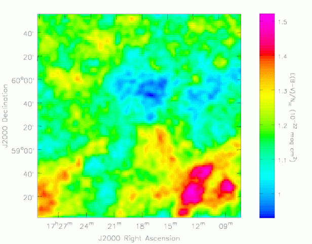
Figure 10: A map of the ratio of reddening to H I, $E(B-V)/N_{\rm HI}$, over the FLS field. The reddening is from Schlegel, Finkbeiner, & Davis (1998) smoothed to the angular resolution of the H I data, and the H I is for $T_{s}=80$ K and omits emission associated with the high-velocity cloud. Areas with the highest ratios are generally not those with the largest $N_{\rm HI}$ but those with the largest $T_{\rm b}(V)$: the largest $N_{\rm HI}$ occurs in the upper left of the map (see Fig. 8), a region of average $E(B-V)/N_{\rm HI}$, while the most dust per unit $N_{\rm HI}$ is in the ‘arc’ feature and related emission at the lower right.

Figure 11: The ratio $E(B-V)/N_{\rm HI}$ for $T_{s}=80$ K, vs. the peak brightness temperature in the H I line. To reduce clutter only every second point is plotted. When the 21cm spectrum has a component with $T_{b}\gtrsim 12$ K, the reddening per H I atom is higher than the average value, $1.2\times 10^{-22}$ mag cm², found for the most transparent lines of sight. This suggests that for $T_{\rm b}>12$ K the derived value of $N_{\rm HI}$ is not representative of the true $N_{\rm H}$ because H I is cooler than the assumed $T_{s}=80$ K, or because that direction contains some $H_{2}$.

Table 1: GBT H I Map of the FLS Field

Field Center (J2000)	$17^{\rm h}18^{\rm m}+59\arcdeg 30\arcmin$
Field Center (Galactic)	88$\fdg$32 +34$\fdg$89
Map Size (J2000)	$3\arcdeg\times 3\arcdeg$
Effective Angular resolution	$9\farcm 8$
Pixel Spacing	$1\farcm 5$
$V_{\rm LSR}$ Coverage (km s-1)	$-314$ to $+213$
Velocity Resolution	0.62 km s-1
Channel Spacing	0.52 km s-1

Table 2: Uncertainties in the Final Data

Noise	0.08 K ($1\sigma$)
Stray Radiation	0.1 – 0.25 K ($1\sigma$)
Total $N_{\rm HI}$ error	$1.1\times 10^{19}$ cm-2 ($1\sigma$)

Table 3: H I Features in the FLS field

Object	$\alpha,\delta({\rm J2000})$	Peak $N_{\rm HI}$	$V_{\rm LSR}$	FWHM
		(cm-2)	(km s${}^{-1})$	(km s-1)
(1)	(2)	(3)	(4)	(5)
Complex C	$17^{\rm h}15^{\rm m}00^{\rm s}+60^{\circ}09^{\prime}$	$6.9\times 10^{19}$	$-190$	20.0
IVC 1	$17^{\rm h}22^{\rm m}28^{\rm s}+60^{\circ}30^{\prime}$	$5.6\times 10^{19}$	$-41$	5.1
IVC 2	$17^{\rm h}23^{\rm m}24^{\rm s}+59^{\circ}58^{\prime}$	$5.0\times 10^{19}$	$-41$	5.3
IVC 3	$17^{\rm h}27^{\rm m}39^{\rm s}+58^{\circ}06^{\prime}$	$4.4\times 10^{19}$	$-34$	15.8
IVC 4 (Draco)	$17^{\rm h}11^{\rm m}16^{\rm s}+60^{\circ}40^{\prime}$	$7.8\times 10^{19}$	$-23$	5.4
Arc	$17^{\rm h}10^{\rm m}30^{\rm s}+58^{\circ}41^{\prime}$	$1.8\times 10^{20}$	$-2$	2.7

Note. — The quantities refer to the direction of greatest $N_{\rm HI}$.

Table 4: Statistics on total $N_{\rm HI}$ ($T_{\rm s}=80$ K) across the FLS Field

Area	$N_{\rm HI}\ (10^{20}$ cm${}^{-2})$
(deg2)	min	max	avg	Std Dev
(1)	(2)	(3)	(4)	(5)
0.02			2.36
1	1.8	3.1	2.51	0.28
4	1.8	3.2	2.45	0.25
9	1.7	3.9	2.48	0.32

Table 5: $E(B-V)=a_{0}+a_{1}N_{\rm HI}$  (for T${}_{s}=80$ K)

H I Velocity Range	$E(B-V)$	a0	a1	Std. Dev.
(km s-1)	( mag)	($10^{-3}$ mag)	$(10^{-22}$ mag cm2)	($10^{-3}$ mag)
All	All	$1.7\pm 0.8$	$1.0\pm 0.03$	$3.5$
$>-$$100$	All	$-7.3\pm 0.4$	$1.5\pm 0.02$	$2.0$
$>-$$100$	$<$$0.03$	$-2.1\pm 5.0$	$1.2\pm 0.02$	$1.6$

Note. — Error estimates are $\pm 1\sigma$ from the least squares fit.

References

- Bohlin, Savage, & Drake (1978) Bohlin, R. C., Savage, B. D., & Drake, J. F. 1978, ApJ, 224, 132
- Boulanger & Perault (1988) Boulanger, F., & Perault, M. 1988, ApJ, 330, 964
- Boulanger et al. (1996) Boulanger, F., Abergel, A., Bernard, J.-P., Burton, W. B., Deśert, F.-X., Hartmann, D., Lagache, G., & Puget, J.-L. 1996, A&A, 312, 256
- Boulanger et al. (2001) Boulanger, F., Bernard, J-P., Lagache, G., & Stepnik, B. 2001, in “The Extragalactic Infrared Background and its Cosmological Implications”, IAU Symp. 204, ed. M. Harwit & M.G. Hauser, ASP, p. 47
- Burrows & Mendenhall (1991) Burrows, D. N., & Mendenhall, J. A. 1991, Nature, 351, 629
- Condon et al. (2003) Condon, J. J., Cotton, W. D., Yin, Q. F., Shupe, D. L., Storrie-Lombardie, L. J., Helou, G., Soifer, B. T., & Werner, M. W. 2003, AJ, 125, 2411
- Deul & Burton (1990) Deul, E. R., & Burton, W. B. 1990, A&A, 230, 153
- Dickey & Lockman (1990) Dickey, J. M., & Lockman, F. J. 1990, ARA&A, 28, 215
- Gladders et al. (1998) Gladders, M. D. et al. 1998, ApJ, 507, L161
- Hartmann et al. (1996) Hartmann, D., Kalberla, P. M.W., Burton, W. B., & Mebold, U. 1996, A&AS, 119, 115
- Hartmann & Burton (1997) Hartmann, D. & Burton, W. B., 1997, “Atlas of Galactic Neutral Hydrogen”, Cambridge University Press (the LD survey)
- Hauser (2001) Hauser, M. G. 2001, in ”The Extragalactic Infrared Background and its Cosmological Implications”, IAU Symp. 204, ed. M. Harwit & M.G. Hauser, ASP, p. 101
- Heiles, Reach, & Koo (1988) Heiles, C., Reach, W.T., & Koo, B.-C. 1988, ApJ, 332, 313
- Heiles, Haffner, & Reynolds (1999) Heiles, C., Haffner, L.M., & Reynolds, R.J. 1999, in New Perspectives on the Interstellar Medium, ed. A.R. Taylor, T.L. Landecker, & G. Joncas, ASP Vol. 168, 211
- Herbstmeier et al. (1996) Herbstmeier, U., Kalberla, P. M. W., Mebold, U., Weiland, H., Souvatzis, I., Wennmacher, A., & Schmitz, J. 1996, A&A, 117, 497
- Higgs & Tapping (2000) Higgs, L. A., & Tapping, K. F. 2000, AJ, 120, 2471
- Jewell (2000) Jewell, P.R. 2000, in Radio Telescopes, Proc. SPIE Vol. 4015, 136
- Kalberla, Mebold, & Reich (1980) Kalberla, P. M. W., Mebold, U. & Reich, W. 1980, A&A, 82, 275.
- Kalberla, Mebold, & Reif (1982) Kalberla, P. M. W., Mebold, U., & Reif, K. 1982, A&A, 106, 190
- Lagache et al. (1999) Lagache, G., Abergel, A., Boulanger, F., Désert, F.X., & Puget, J.-L. 1999, /aap, 344, 322
- Lagache et al. (2000) Lagache, G., Haffner, L.M., Reynolds, R.J., & Tufte, S.L. 2000, /aap, 354, 247
- Liszt (1983) Liszt, H.S. 1983, ApJ, 275, 163
- Liszt (2001) Liszt, H. 2001, A&A, 371, 698
- Liszt (2002) Liszt, H. 2002, A&A, 389, 393
- Liszt & Lucas (2000) Liszt, H., & Lucas, R. 2000, A&A, 355, 333
- Lockman, Jahoda, & McCammon (1986) Lockman, F. J., Jahoda, K., & McCammon, D. 1986, ApJ, 302, 432
- Lockman (1998) Lockman, F. J. 1998, in Advanced Technology MMW, Radio, and Terahertz Telescopes, SPIE Vol. 3357, 656
- Lockman (2003) Lockman, F. J. 2003, in Single Dish Radio Astronomy: Techniques and Applications, ASP Conf. Ser. 278, ed. S. Stanimirovic, D. R. Altschuler, P. F. Goldsmith, & C. J. Salter, (San Fransisco: ASP), 397
- Lockman (2004) Lockman, F. J. 2004, in Soft X-Ray Emission from Clusters of Galaxies and Related Phenomena, ed. R. Lieu & J. Mittaz, Kluwer, p 111.
- Miville-Deschen̂es et al. (2003) Miville-Deschen̂es, M.-A., Joncas, G., Falgarone, E., & Boulanger, F. 2003, A&A, 411, 109
- Norrod & Srikanth (1996) Norrod, R., & Srikanth, S. 1996, NRAO GBT Memo Series No. 155
- Penprase, Rhodes, & Harris (2000) Penprase, B. E., Rhodes, J. D., & Harris, E. L. 2000, A&A, 364, 712
- Rachford et al. (2002) Rachford, B.L., Snow, T.P., Tumlinson, J., Shull, J.M., Blair, W.P., Ferlet, R., Friedman, S.D., Gry, C., Jenkins, E.G., Morton, D.C., Savage, B.D., Sonnentrucker, P., Vidal-Madjar, A., Welty, D., & York, D.G. 2002, ApJ, 577, 221
- Reach, Koo, & Heiles (1994) Reach, W.T., Koo, B.-C., & Heiles, C. 1994, ApJ, 429, 672
- Savage et al. (1977) Savage, B.D., Bohlin, R.C., Drake, J.F., & Budich, W. 1977, ApJ, 216, 291