A Search for Variable Stars and Planetary Occultations in NGC2301 I: Techniques

Abstract

We observed the young open cluster NGC 2301 for 14 nights in Feb. 2004 using the orthogonal transfer CCD camera (OPTIC). We used PSF shaping techniques (“square stars”) during the observations allowing a larger dynamic range (4.5 magnitudes) of high photometric precision results ($\leq$2 mmag) to be obtained. These results are better than similar observing campaigns using standard CCD imagers. This paper discusses our observational techniques and presents initial results for the variability statistics found in NGC 2301. Details of the variability statistics as functions of color, variability type, stellar type, and cluster location will appear in paper II.

1 Introduction

The study of stellar variability has long been a part of astronomical research and is the mainstay for understanding stellar evolution, stellar formation, stellar death, and galactic dynamics. Variable stars are fundamental to such astrophysical pursuits as composition of the ISM, evolution of galaxy clusters, and cosmological distance scales. Two areas of variability have been ignored by most astronomers using large telescopes (due to lack of sufficient observing time, lack of the proper instrumentation, and/or insufficient photometric precision); low amplitude variations ($\sim$0.1 mag or less) and frequent time sampling for extended periods (i.e., few minute sampling for many days in a row). Studies of these two regions of phase space, when tied together with large areal surveys or dense stellar regions, are also capable of providing detections and limits on the number and type of transiting extra-solar planets encircling solar-type stars.

An initial study reaching high photometric precision and large area was presented in Everett et al., (2002) and Everett & Howell (2001). The latter paper also presents a brief review of other similar variability studies. The Everett et al., study concentrated on field stars covering a large range of color and luminosity class. Here, we present a similar high photometric precision study of 0.15 sq. degrees centered on the young, metal rich star cluster NCG 2301. This paper outlines the novel observational technique we used and details the new data reduction and analysis applied to the nearly 5000 (mostly solar-type stars) light curves we collected over a 14 night period in Feb. 2004. Paper II will provide details of the stars themselves, their light curves, and a discussion of how this study reveals new insights into open clusters and NGC 2301 itself.

2 Observations

2.1 High Precision Photometry

The accuracy of any observation is ultimately limited by photon statistics (assuming one can control other factors, especially systematic noise), which for stellar sources is approximately the peak count in electrons per pixel times the area of the point spread function (PSF). Typical CCDs can collect 30,000 to 100,000 e^- per pixel prior to the onset of non-linearity or full well, and our desired accuracy of 1 millimag (mmag) per exposure can therefore be achieved with a PSF which is at least 3–6 pixels FWHM. However, if we are trying to simultaneously observe many stars over a wide range of apparent magnitude with a precision of 1 mmag, we must collect $10^{6}$ e^- from the faintest stars without saturating the brightest ones. For example, if we want to maintain precision over 5 magnitudes, we require a PSF of FWHM 30-60 pixels. Of course this incurs a penalty of increased photon statistics from sky noise, and increased systematic error from overlapping PSF but these considerations are factored into the decision about the optimal PSF size to use.

One way of achieving the above scenario is to defocus the telescope, but this causes difficulties because the “donut” PSF is not constant across the image, causing problems with photometry from PSF fitting which is essential because of overlapping stellar images. Additionally, defocused images often place power in very extended, asymmetric wings of the PSF and highlight optical imperfections. Creating a large PSF in order to sample as much of the stellar apparent magnitude range as possible, sampling as large a field of view as possible, and at the same time as trying to achieve extreme (mmag) photometric accuracy are conflicting requirements with defocussed images. Obviously the quantitative level one can attain with defocussed images depends on the specifics of the telescope, detector, cleanliness of optics, etc, but at the UH2.2-m telescope, for example, there is enough vignetting over our 10^′ field of view that trying to fit defocussed images with a constant PSF leads to systematic errors well in excess of 1 mmag. We have chosen to exploit the capabilities of orthogonal transfer CCDs and rapidly raster scan the stellar images over a square PSF during the course of an exposure. Initial work on this type of “square star” photometry is discussed in Howell et al., (2003). We were not completely successful in reaching photon-limited performance for reasons discussed below, but we believe that this technique could do so with some refinement.

Square star production allows us to control the size and shape of the extended PSF however, they are not a perfect solution to all types of observing. For example, field crowding can become an issue, very faint background stars incur additional uncertainty from increased sky signal, and two-dimensional objects, such as galaxies, are rendered unusable for most purposes. Also, the square star resides in more pixels than a traditional round star would, thereby bringing additional read noise (and dark current if an issue) into play. This increased noise is not of real concern here however, as we are working in the regime of stellar photon noise being the dominant source of uncertainty.

2.2 The Field

There is an optimal stellar density to survey many stars at once. Obviously a very low stellar density nets us very few stars per exposure, whereas a very high density causes us problems from overlapping images. A simple calculation reveals that the greatest number of non-overlapping stellar images which are found at random locations is $N/(en)$, where $N$ is the number of pixels in the detector, $n$ is the number of pixels in the PSF, and $e$ is the base of natural logarithms. Of course the real situation is more complicated because we can tolerate overlaps to some degree and a range of stars of very different brightnesses which affect the ability to extract photometry from close stars. Even so, this indicates that for a camera such as OPTIC, which has $4096^{2}$ pixels and a PSF which we fix at $30^{2}$ pixels, to sample 5 magnitudes of stellar brightness, we ought to aim for a stellar density which gives us at least 10,000 stars over the full range of apparent magnitude of interest. This is a higher density than we could actually achieve, given the rather small pixel size ($0.138$^′′). (We had hoped to employ a focal reducer at the 2.2-m telescope, but it was not ready in time.) Obviously we could push the density of stars with $10^{6}$ photons as high as we like by extending the observing time, but this has to be traded off against the sampling frequency of several times per hour which we wanted to search for planets.

We searched the USNO-B catalog over those right ascensions available for our time allocation of first half nights in February, looking for fields which offered high stellar density, good visibility over most of the night, and slanted toward a high likelihood field of view to detect transiting planets. We choose to center our survey on the young (164 million years), open Galactic cluster NGC 2301. This cluster is of high metallicity (+0.06), 872 pc away, and has a low reddening (0.028 mag). The distance modulus to NGC 2301 is 9.79 making the turnoff magnitude (near main sequence spectral type A0) occur at R=10, or just below our saturation limit. We therefore did not collect valid photometric time series data on any evolved higher mass main sequence stars (i.e., giants) but did find two stars that have apparently already passed into the white dwarf stage. It would have been possible to reach a higher density in the center of a globular cluster, but not over multiple 10^′ fields of view, and we did not want to look for planets in such an environment.

2.3 The Observing Run

We were granted the first half of 14 nights at the UH 2.2-m telescope atop Mauna Kea by the UH TAC: 09-Feb-2004 through 22-Feb-2004. Two of these nights were completely lost to bad weather, two were curtailed from the time-series program to collect calibrated photometry (B,R) and photometric calibration information, but the remainder of the time was spent moving rapidly between six adjacent fields around NGC 2301 (see Figure 1). A typical cycle would involve scripted, automatic telescope offset to the first field, acquisition of guide star, a 120 s exposure in $R$ band, approximately 60 s for readout and offset to the next field, for a net duty cycle of 2/3. We therefore cycled through the six fields in approximately 16 minutes, revisiting each star that often. Since we were allocated half nights, we could manage 5–6 hours on target, depending on how quickly after sunset we were willing to start (our first observations of each night generally show distinctly worse residuals because of the brighter sky), and we accumulated an average of 17 cycles over all six fields on each of our 10 full nights.

Figure 1: The six OPTIC fields in the cluster are shown by plotting the locations of the stars in this study. There is some overlap in the fields and we designate the fields as C, N, S, E, W, and SE (for Center, North, etc.) We guided each exposure using the lower left on-chip guide region in each field which accounts for the slight asymmetry in each OPTIC field.

The observations were made using the OPTIC camera, the prototype and only operating orthogonal transfer CCD camera. OTCCDs allow the collected charge to be moved within the array in response to either on-chip guide stars or at the user’s whim in pre-determined patterns. Based on the experience gained in our previous observations with these types of CCDs and OPTIC (Tonry et al. 1997; Howell et al. 2003), we decided to undertake a comprehensive variability study using shaped stars. While promising in initial tests, the challenges of using this new technique in a relatively crowded field, over many nights and converting our reduction techniques to deal with square stars while keeping high photometric precisions were non-trivial.

The observations were all taken with a $30\times 30$ pixel raster pattern applied to the accumulating charge in the CCD, relative to the light from the stars which was kept fixed on the CCD by guiding on a selected star in an unshifted guide region. This raster scan was carried out 5 times during the 120 s exposure, with a typical guide rate of 12 Hz, so the 900 pixels within the $30\times 30$ raster pattern were swept over in about 288 steps, amounting to approximately a 3 pixel ($\sim$ 0.5 FWHM) charge shift per guide iteration. See Howell et al. (2003) for details.

In addition to the square star observations, we also took focused, non-rastered images in $B$ and $R$ with exposure times of 2, 5, 10, 15, 50, 100, 150, and 300 seconds to establish astrometric and photometric measures for our stars. After flattening, these images were each run through the DoPhot program (Schechter et al. 1993) to identify the stars present and measure their fluxes. Another program then took the DoPhot output files and matched up all the stars between pairs of images (some pairs with extremely different exposure time had no overlap). The median magnitude difference was calculated for each pair, the ensemble of differences placed in an antisymmetric matrix, the distribution quartiles in an accompanying error matrix, and the whole solved for a vector of photometric offsets between the different exposures. This enabled us to get relative magnitudes in $B$ and $R$ between $10<R<20.5$ and $10<B<22)$ with internal error less than 0.01 mag. Comparison of the applied R time series magnitudes to constant stars in the field overlap regions also showed that we obtained internal photometric calibrations across fields to 0.01-0.02 magnitudes for our brightest 6 magnitudes of stars. On a relatively photometric night we observed Rubin-152 at a variety of airmasses, which established our photometry zero points in $B$ and $R$ to about 0.025 mag, and permitted us to put all our B and R magnitudes were then set on a standard photometric scale.

Figure 2 shows our color-magnitude diagram (CMD) for NGC 2301. The main sequence for NGC 2301 is very apparent and broadened due to binaries within the main sequence stars. Our time series observations, which saturate at $R<10$, do not quite reach the cluster turnoff at R$\sim$10 but do reveal 2 new white dwarf candidates. This is a somewhat surprising result due to the young age of this cluster as only stars earlier than about A0 can have evolved this far. Spectroscopic and cluster membership confirmation for these sources are planned. The lower right hand corner of Figure 2 shows that a number of stars (late K and M) are still evolving to the main sequence in this young cluster. We also note the dense distribution of stars lying below and to the left of the main sequence starting near $R\sim 16.5$ which are most likely non-cluster contaminates.

Figure 2: Color magnitude diagram for NGC2301. This CMD combines all our stars from the six fields. Note the broadening of the main sequence due to non-cluster member contamination (blue side below R$\sim$16.5) and the lower pre-main sequence stars lying above the ZAMS. The brightest stars we have valid data for are near the cluster turn-off at an absolute magnitude near 0.

In order to provide positions for each of our program objects, we performed astrometry using our non-rastered images (i.e., normal type CCD images with round stars taken with the same camera and telescope and used for the B,R calibration). Calculating astrometric positions for the stars was straightforward. We extracted stars from the USNO-B catalog within 50^′ of our field center, which distilled down to about 1700 stars encompassing each of the six fields. OPTIC has two CCDs, so we matched the DoPhot coordinates for both CCDs independently in each of the six fields to the USNO-B stars using Brian Schmidt’s “starmatch” program. A simple cubic fit to the stars with matched CCD and USNO-B coordinates then gave us the means to get from CCD coordinates to RA and Dec. As usual, the coordinates we generate therefore have the high relative precision of CCD astrometry and the good, averaged absolute precision of the USNO-B catalog. We expect that the relative positional uncertainty of our coordinates is something like 0.1 pixel (15 mas) since all of our stars are bright, and the absolute positional uncertainty is limited by USNO-B at something like 100 mas.

2.4 The Reductions

Data taken with orthogonal shifting are smoother than conventional CCD data because each bit of sky is integrated on a set of CCD pixels. However, this means that each observation must have a custom flat field constructed by convolving an unshifted flat field with the shift pattern of each image. This was done for all observations, and each bias-subtracted data image was divided by its flat field.

Using the very deep, complete list of stars from the photometry observations, we assembled an empirical PSF for each image by selecting “reasonably isolated” stars and adding their images together and subtracting the overlaps from nearby stars. Specifically, any star which has a neighbor brighter than half its flux closer than 100 pixels, or is contaminated by masked pixels, or has a mean flux greater than 30,000 or less than 10,000 ADU per pixel, or is too close to the edge of the chip was rejected. The rest contributed to a linear fit between mean brightness of the PSF “mesa” and flux expected from the photometry file. This fit was analyzed to identify stars which were saturated or otherwise outliers, and the remainder form the list of final contributors. The fit was also used to set the scale factor between DoPhot fluxes and star fluxes in this observation. The square image created by each contributor star was shifted by the closest integer offset into alignment and a subarray of size $\approx 60$ pixels around each added. The PSF from the previous iteration was then multiplied by the tabulated fluxes for all stars, and any overlapping data from the contributing stars was subtracted. This procedure was then iterated 10 times.

Experiments reveal that the fractional pixel position errors are an insignificant contributor to error in the eventual fluxes which are derived from these PSF subarrays. However, we encountered an unanticipated problem which limits our photometry to about 1 mmag at best and more like 2 mmag typically. The problem is that we shift the charge relative to the stars at a rate of about 5^′′/sec, and this unfortunately means that we are moving the seeing disk of the stellar images by about the seeing diameter during the time the seeing changes size and shape and scintillates due to atmospheric turbulence. Faster shifting would smear out these effects; slower shifting would cause them to integrate out more. As it is, our PSF mesas have slightly corrugated tops and these corrugations change markedly across the 9.2^′ field of view, although they correlate well for nearby stars (within $\sim$2 arc min). The average PSF we have assembled does not match the individual stars perfectly, leaving behind seeing-sized bumps which are at a level of a few $10^{-4}$ of the original flux. There are perhaps 30–50 independent 0.6–0.8^′′ bumps across the $30\times 30$ pixel ($4\times 4$^′′) PSF which leads to an error which is of order $10^{-3}$. In principle it would be simple to blur out this effect by shifting much faster during the exposure (we could potentially work at 2000^′′/sec). We could also do a more careful data analysis which would involve using local PSF stars (within $\sim$2 arc-minutes) to analyze their own neighborhoods (see Everett & Howell 2001). For the purpose of finding extra-solar Jupiters causing 15 mmag extinction and a variable star census, however, we are temporarily satisfied with a 1-2 mmag error floor.

Once an image has a PSF subarray extracted, the flux analysis is relatively simple. Stars which are fainter than some limit according to the photometry list are simply removed from the image by scaling the PSF to their flux and subtracting. This limit was 300 $e-$/sec summed over the entire PSF for the flux, which is approximately $R=19.4$, depending on conditions. There are typically 600–700 stars remaining in each of our fields brighter than this, and we do a simultaneous least squares fit for the brightness and sky level of each star. The fit produces quantitative covariances for overlapping stars, of course, but to date we have ignored this information except to delete stars with more than 10% neighbor contamination from the variability statistics below. We would be happy if uncertainty were limited by the photon statistics, but this does not happen for stars which are brighter than about $R\sim 17$ or 3000 e^-/sec total (i.e. for which the uncertainties should be less than 1.7 mmag). We therefore estimate an uncertainty for each star by examining the rms residual after subtracting the PSF fit, and multiplying by the square root of the number of independent seeing footprints within the square PSF.

Figure 3 shows $\chi^{2}$ per degree of freedom for stars from a typical observation, illustrating how it worsens for $R<17$, and Figure 4 shows that the typical uncertainty in the differential light curves for all our stars bottoms out around 1–2 mmag at $R<17$ rather than continuing to plummet according to photon statistics. This property of the residual uncertainty is an important advantage of our square star photometry method. Our best photometric statistics apply over a flat linear regime covering 4-5 mags whereas typical CCD photometry follows closely the “S/N” equation yielding the best photometry for the top 1-2 mags only and then falling away (see e.g., §4.4 in Howell 2000 and Fig. 3 in Everett & Howell 2001). The smaller dynamic range in normal CCD observations even holds true for relatively large defocused images (e.g., Gilliland et al., 1993).

Figure 3: $\chi^{2}/N$ for stars from a typical observation. The fitting statistics begin to degrade near R=17.

Figure 4: Photometric uncertainty for the stars in our sample. $\sigma$ is the standard deviation of the entire light curve for each point source. Note the relatively flat error response from R=11.7 to R=16.5.

The final step necessary is to bring all of the observations onto a common zero point, since atmospheric extinction and occasional haze or cloud obviously change the flux zero point. This is accomplished by a similar fit procedure to that of the photometry observations. All the observations ($\sim 170$) for a given field are read and all the stars ($\sim 1200$) in that field for which there are flux measurements are matched up. For each pair of observations, stars with $12.9<R<16.4$, which have $\chi^{2}/N<20$, and which have few masked pixels are compared with the median magnitude difference and quartiles contributing to antisymmetric and symmetric matrices. These are again analyzed as pairwise differences of an offset vector, and the offset vector is applied to bring the observations into agreement. This is done once for each entire field; stars which have quartile variability greater than 2.5 mmag are deleted; and the fit is redone for each quadrant (amplifier) of the OPTIC field. The final zero point is set by the photometric observation list.

Figures 5 and 6 illustrate what the final data look like. Figure 5 shows a star in the middle of our magnitude range which has little or no statistically significant variability which we can detect. We believe this is representative of what our data can reveal when a star’s luminosity is constant. The half-range between quartiles for the magnitude distribution (hereafter called “quartiles”, approximately a factor of 1.5 smaller than $1\sigma$ for a Gaussian distribution) is 1.0 mmag.

Figure 5: Light curve for an $R=14.4$ star for which we do not see statistically significant variability. The uncertainties for this star are 1$\sigma$$\sim$0.0032 mag, comparable to the scatter, with apparent low-level systematics visible from day to day.

Figure 6 shows three variable stars whose periods are nicely covered by this study. The quartile residuals of the two brighter stars are about 2 mmag, and the light curve amplitudes are evidently approximately 0.06 mag. Figure 7 shows the observations of the top star in Fig. 6 phased around its period.

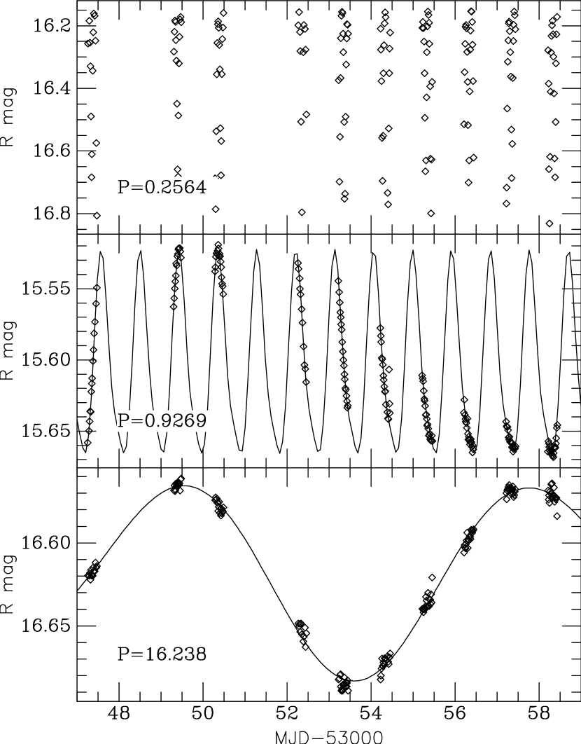
Figure 6: Light curves for three variable stars spanning a range in period (given in units of days).

Figure 7: Light curve for the short period (contact) eclipsing binary star (top of Figure 6), phased on its period.

In order to see if our limiting photometric precision could be due to color terms in the data, we performed the following test. Keep in mind that there are two main steps in our processing where uncertainties can creep in. One is the determination of the stellar fluxes and the other is the use of ensembles of the brightest stars to determine the point-to-point magnitudes in each light curve. For our flux determination, we used a single model square star “PSF” to determine all the stellar fluxes in each quadrant of the OPTIC field of view. We have already discussed how this was a source of small uncertainties as the detailed shape of the “top” of the mesa changed across the field. Given this level of uncertainly, we want to investigate if the intrinsic color of any given star causes an additional uncertainty in its brightness determination.

Everett and Howell (2001) discuss this point somewhat but do not present detailed information to substantiate their findings. The reason is that when making stellar ensembles to test blue vs. red ensembles used to perform differential photometry on say red and blue stars, one finds that there are often not enough blue stars in a local region and using a larger part of the field of view introduces additional uncertainty. In addition, the fainter stars are usually the reddest and building a fairly red ensemble to use on say the reddest stars also has lower precision automatically as it starts with stars of higher uncertainty. The test we tried here is to use the likely random placement of stars of various colors to build local ensembles across the entire field of view of each of the six regions. We broke up each field of view into 36 boxes in a 6x6 pattern. In each box, an ensemble was chosen consisting of the brightest stars. Each ensemble was subjected to the tests for ensemble stability as described in Everett & Howell (2001). In some cases, the boxes had too few stars or too few that made good ensemble members so we were forced to combine adjacent boxes together. For the more crowded center region (region C) we ended up with 33 different groups of stars and 15-20 groups in the other regions.

Comparison of the resulting light curve uncertainties using this technique with the light curve uncertainties based on the procedure described above shows that the smaller areal ensembles produce, on average, light curves with 10-15% better uncertainties. We find, however, no differences in the mean uncertainties of the light curve variances across the field of view or from group to group. One assumes that some of the ensembles are likely biased toward the red and are used on blue stars and vice verse. Thus, to the best we can tell the use of more local ensembles, while having the issue of total numbers of good stars available and an increased data reduction effort, allows for slightly better average precisions, but we find no evidence that differential color terms come into play.

An additional point in support of not seeing color term effects is that we do not find the highest level of variability to occur in the stars with the most extreme colors (see Paper II). Everett et al., (2002) present histograms of variability as a function of stellar color and indeed they find a higher percentage of variables at the bluest ($B-V\sim 0.25$) and reddest ($B-V\sim 1.3$) colors. However, the increase in percent is marginal at best at the red end (actually more like the mean of the distribution and only an apparent increase over a low level at $B-V\sim 0.5$) and the blue increase (which shows larger error bars due to low number statistics) is due entirely to pulsational variables ($\delta$ Sct and SX Phe types) and not color terms. While the effect of differential color due to atmospheric extinction changes and over time (airmass) are likely to be present at some level, it appears that to at least 1 mmag they are averaged out through the use of local ensemble differential photometry. It may be that they are averaged out at even higher precision levels as well. Howell & Tonry (2003) have obtained time series observations reaching a precision of 0.5 mmag with no apparent color term variations, although the total range of stellar color in the study was smaller than that used here.

3 Analysis

For the purpose of finding planets and identifying variability, we assembled some statistics for each light curve. The first is simply the median magnitude and quartiles. The second pair of statistics are the “low-pass” and “high-pass” variability indices. The first is the quartiles of the median magnitude for each day, which will flag light curves which vary on timescales of days or longer. The second is the median of the quartiles for each day considered separately, which will flag light curves which vary significantly within a day. The third pair of statistics are designed to identify planets. “extreme” is the most extreme excursion of a day’s median from the overall median. “badday” is the quartile for the single day with the largest quartile variability. The planet search strategy is to find a star with small “high-pass” but with a big “badday” which might signify a 15 mmag eclipse which took place.

3.1 Occulations

Experiments with inserting a 15 mmag eclipse demonstrated that such an event would clearly stand out in our statistical tests. We were particularly interested in periods of $\sim 4$ days since they would potentially give us the opportunity of seeing more than eclipses, and a Jupiter-sized planet would give us a 15 mmag dip, so we inserted eclipses corresponding to orbits of radius $\sim 0.06$ AU with random phasing into light curves. A shortcoming to our “1/2 night” survey is that by covering only quarter days during this two week observing run, something like 1/2 to 2/3 of planets with $\sim 4$ day periods would simply fall between the cracks. Nevertheless, with favorable phasing a planet causing a 15 mmag eclipse every few days would stand out very clearly in the parameter-parameter distributions described in the previous section. The rank of such artificial eclipses in terms of separation from the mean parameter correlations was around the 99th percentile, so it was a simple job to examine such light curves by eye and decide whether the event looked like an eclipse or not. All artificially inserted eclipses were readily identified.

However, examination of all light curves with potentially real planetary occultations revealed none which was a good transit candidate, at least at the 10 mmag level. A zero discovery rate is not out of line with present-day extra-solar planet statistics and estimates of their discovery rate (Howell et al., 1999) given our short observing time interval. An interesting reason for rejection of most is the fact that the variations in magnitude occurred primarily on time scales much shorter than those associated with the expected transits. The sample we have in this study contains mostly solar type stars and of these, many appear to be fairly active (rotational and spot modulations), thus possibly presenting a challenge to transit hunters.

Carpano et al. (2003) and Jenkins (2002), and others, discuss methods of searching for planetary transit signals amoung highly variable light curves, specifically those associated with active or rapidly rotating solar-like stars. These authors bascially convolve matched filters (i.e., known transit shapes, depths, and durations) with pre-whitened (often high S/N) light curves. The methods they use, detailed filtering of the light curves to remove frequencies which contaminate them but are unrelated to transits, plus the possible additional use of color information appear to be possible, in theory, for transit detection (although yet to be realized in actual data). However, our dataset, and most obtained at present by planet hunters, has neither the time sampling, time duration, or color information (or a combination of these) to try such techniques.

3.2 Stellar variability

Figure 8 illustrates the variability we see in the light curves of all the stars for which we measured time series fluxes. The abrupt upturn in variability at $R<11.5$ signifies the onset of saturation, and the errors from photon statistics become apparent at $R>17$. At the 3$\sigma$ level, we find that 56% of all our point sources (over all magnitudes) are statistically variable. While a small percentage of these variables may be due to remaining low-level systematic effects, we believe that a 3$\sigma$ cutoff is a conservative estimator. Of all the variables, 64% (at a 99% confidence level) are periodic with periods from $\sim$20 minutes to many days. This number was determined by applying a period fitting routine (PDM; Stellingwerf 1978) to each total light curve and listing a star as variable if it had a determined period at the 99% or higher confidence level. The full details of the variability nature of NGC 2301, how it manifests itself in terms of stellar type and brightness and location within the CMD, will be discussed in paper II.

Figure 8: Quartile variability for all stars as a function of their $R$ magnitude. The top and bottom panels show the same points at different scales. We again see the large dynamic range of “good” data and the eventual degradation starting near R=17.

For the purposes of more fully understanding the statistics of stellar variability in this cluster and in our survey, we work with a smaller sample, restricted to the 5 magnitudes between $12<R<17$. Both Fig 4 and Fig 8 assure us that our observational errors in these regions are approximately 2 mmag or better. There are 1148 out of 4462 stars in our sample which meet this criterion. (Restricting the data to the 661 stars with $12<R<16$ does not affect the conclusions below.)

We note here that typically stars with “low-pass” $>$ “high-pass” variability are textbook variable stars with periods of days to weeks. Some stars with “low-pass” $<$ “high-pass” have periodic light curves with periods which are a fraction of a day, but for the most part they show no obvious periodicity, sometimes with episodic flares or eclipses, but usually just “grumbly” light curves which wander around with quartiles at the 5-10 mmag level.

Figure 9 illustrates the overall level of quartile variability among this sample of stars. The data are well described by a power law of slope $dN/dx=x^{-2}$, where $x$ is the quartile variability. This $N(x)$ diverges at $x=0$, of course, but if restricted to $x>1.6$ mmag the cumulative fraction of stars with quartile variability $x$ mmag or less is

$$f(<x)=1-{1.6~{}\hbox{mmag}\over x}$$ (1)

Figure 9: Fraction of the sample displaying variability is shown as a function of quartile variability amplitude. The small points are variability bins of 1 mmag; the large points are variability bins of 20 mmag; the straight line is a power law of slope $-2$.

The distribution shown in Figure 9 reveals a surprising level of variability among stars. (Recall that this is quartile variability, 1.5 times smaller than $\sigma$ for a Gaussian.) For example, the median quartile variability amplitude in our data (including both periodic and non-periodic sources) is 3.2 mmag, and 1/6 of stars have variability greater than 10 mmag. To place this into perspective, we examine the percentage of variability found in two other similar time sampled surveys. Huber et al. (2004) obtained V band time series data consisting of 1-2 nights of 10 min exposures, 1 week of occasional sampling, and a 1 year revisit for 23 sq. degrees of sky located at various Galactic positions. Their photometric precision was near 0.01 mag at the bright end and they found that that 7-8% of the stars they studied (over all magnitudes in the survey) were variable. Everett et al., (2002) obtained 3 minute time sampling of a single 1 sq. degree region for 5 nights in a row with photometric precision near 5 mmag at the bright end. They found 17% of the sources observed to be variable. Our survey reached better photometric precision and kept this precision over a much larger range in magnitude than these previous examples. Thus it appears that the harder you look, the more variability you find.

The distribution of the variability in terms of amplitude, shape of the variations, and type of star is of interest as it may be a critical item which limits photometric searches for small planet-to-host-star ratios as well as transit detection at all. Exploration of variability at levels smaller then 1-2 mmag are being pursued by us and soon projects such as Pan-STARRS and the Kepler Discovery mission (launch in 2007) will be producing photometric precisions near 0.5 mmag to 0.1 mmag per measurement. While “hot Jupiters” orbiting Sun-like stars are presumed to be easy targets since they produce 10 mmag eclipses, smaller planets may be harder to discover, given the observed level of stellar variability.

4 Conclusion

The major goal of this observational work was to test a number of new technological regimes. We ran the entire time-series operation with essentially no observer intervention using scripted observations, predetermined field locations and guide stars, and observational starts from a remote location (Manoa). We also tested the ability of PSF shaping for high precision time-series photometry within a fairly crowded stellar environment and found it to work well. Our photometric results provide a much larger dynamic range of high precision data than ordinary focused, round star observations (nearly 5 mags compared to normally 1-2 mags) and reached toward 1 mmag precisions with the likelihood of better results using modified parameters.

This type of detailed variability study will be carried out at a vastly larger scale by the Pan-STARRS program; thus our work here can be considered a precursor of sorts. Baseline parameters for variability (and constancy) as functions of spectral type, color, etc. as well as data collection and reduction experience will be essential inputs for Pan-STARRS projects.

We have confirmed the use of local ensembles for the highest precision results as put forth by Everett & Howell (2001) and showed that image shape over about a 2 arcmin radius is essentially identical but slight changes are easily noted at 10 arcmin. These changes are caused by the decorrelation of atmospheric distortion with angular separation, and can be improved by different OTCCD shifting strategies.

Our temporal survey of NGC 2301 has revealed a wealth of information on the variability of the cluster stars in terms of spectral type, location in the CMD, type and amplitude of variability, and other properties. Exploration of such datasets for other clusters with varying age, metallicity, and Galactic location are warranted. As higher precision data is obtained, the number of sources that vary goes up. This work demonstrates that stellar variability exists down to mmag levels, and the fraction of stars which are variable increases inversely as the variability level. Gross planetary eclipses of hot Jupiters at the 10 mmag level will not be difficult to spot, but the grumbly nature of low level variability will make Neptune or Earth-sized eclipses very hard to identify in actual data.

References

- Carpano (2003) Carpano, S., Aigrain, S., & Favata, F., 2003, A&A, 401, 743
- Everett (2001) Everett, M. E., & Howell, S. B., 2001, PASP, 113, 1428
- Everett (2002) Everett, M. E., et al., 2002, PASP, 114, 656
- Gilliland (1993) Gilliland, R. L., et al., 1993, AJ, 106, 2441
- Howell (2004) Howell, S.B. & Tonry, J. L., 2003, BAAS, 203, 1707
- Howell (2003) Howell, S.B. et al., 2003, PASP, 115, 1340
- Howell (2000) Howell, S. B., 2000, Handbook of CCD Astronomy, Cambridge, UK, Cambridge University Press
- Howell (1999) Howell, S.B. et al., 1999, ASP Conference Series Vol. 189, p. 170
- Huber (2004) Huber, M. et al., 2004, MNRAS, submitted
- Jenkins (2002) Jenkins, J., 2002, ApJ, 575, 493
- Schechter, Mateo, & Saha (1993) Schechter, P.L., Mateo, M. & Saha, A. 1993, PASP, 105, 1342.
- Tonry (1997) Tonry, J. L., et al., 1997, PASP, 109, 1154