Large scale correlations of quasar polarisation vectors: Hints of extreme scale structures?

Rémi A. Cabanac¹, Damien Hutsemékers², Dominique Sluse², Hervé Lamy³

Abstract

A survey measuring quasar polarization vectors has been started in two regions towards the North and South Galactic Poles. Here, We review the discovery of significant correlations of orientations of polarization vectors over huge angular distances. We report new results including a larger sample of the quasars confirming the existence of coherent orientations at redshifts $z>1$ .

¹ Canada-France-Hawaii Telescope, 65-1238 Mamalahoa Highway, Kamuela, HI 96743, USA.
²Institut d’Astrophysique et de Géophysique, ULg, Allée du 6 Août 17, B5C, 4000 Sart Tilman (Liège), Belgium.
³BIRA-IASB, Avenue Circulaire 3, 1180 Bruxelles, Belgium.

1. Introduction

Large scale alignments of quasar polarization vectors were uncovered by Hutsemékers (1998), looking at a sample of 170 QSOs selected from the litterature and confirmed later on a larger sample (Hutsemékers & Lamy 2001). The departure to random orientations was found at significance levels small enough to merit deeper investigations. Moreover, these alignments seemed to come from high redshift regions, implying that the underlying mechanism might cover physical distances of Giga parsecs. A large survey of linear polarization was then started, with the long-term goal to characterize better the polarization properties of quasars, and a short-term goal to investigate the reality of the alignments. This work gives a preliminary analysis of the alignment effect for a total sample of 355 quasars, comprising new polarization measurements from observing runs between 2001-2003 and a new comprehensive compilation from the litterature.

2. Sample

The sample was chosen from Véron-Cetty & Véron (2000) and the Sloan Digital Sky Survey. Among possible targets a preference was given to bright extragalactic sources having a higher probability to show stronger polarization: BAL quasars, red quasars. The selection criteria of the sample are detailed elsewhere (Hutsemékers 1998, Hutsemékers et al. 2001, 2004; Sluse et al. 2004). In order to avoid possible contaminations from the interstellar medium of the Galaxy, only the objects at galactic latitude $|b_{gal}|>30^{\circ}$ were selected. Above this galactic latitude the interstellar polarization is smaller (Heiles 2000).

The observations were carried out at ESO La Silla 3.6m EFOSC2 (2001, 2002, 2003) and Paranal VLT/FORS1 (2003), in broad-band $V$ filter, using a Wollaston prism and 4 positions of the half-wave plate to derive Stokes parameters $Q$ and $U$ (Hutsemékers et al. 2004; Sluse et al. 2004). The photometry was done using the procedure defined by Lamy & Hutsemékers (1999). Photon errors on $Q$ and $U$ are $\sigma_{Q}\simeq\sigma_{U}=0.16\,\%$ . The foreground polarization (coming from both the instrument and the interstellar medium) was computed from the observed field stars and subtracted from the quasar polarization. Because this was not possible on every frame, we used Stokes parameters averaged from the field stars observed during the same run. This average polarization is always small : $\overline{q_{*}}\simeq\overline{u_{*}}\simeq 0.1\pm 0.2\,\%$ . Final errors were conservatively derived by quadratically adding photon and foreground errors yielding a total error on the QSO polarization degree ca. 0.2-0.3 %. Finally, because the polarization is a positive quantity only, it is debiased according to the Wardle & Kronberg method (1974). To insure a robust measurement of the polarization direction we include only the objects having a polarization degree of $P>0.6\,\%$ and a maximum error in the polarization position angle of $\sigma_{\theta}<14\,^{\circ}$ .

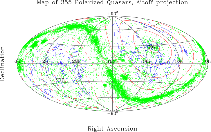
The final sample of polarized quasars comprises 195 quasars in the North Galactic Pole region (NGP) and 160 quasars in the South Galactic Pole region (SGP). Figure 1 shows an Aitoff projection of the full sample superimposed on the galactic star polarization map (Heiles 2000).

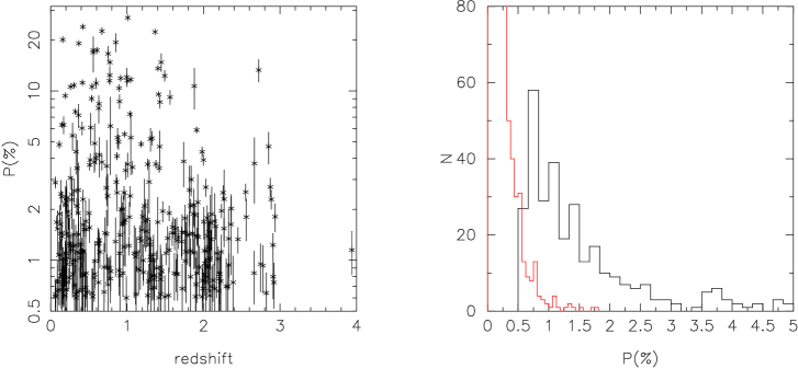
Refer to caption — Figure 1.: Aitoff projection of the full sample of polarized quasars (black segments) and galactic stars (grey segments; Heiles 2000). Contours are 20^∘-step galactic parallels (solid lines towards NGP; dashed lines towards SGP). In polar regions the quasar polarization is on average 5 times stronger than the star polarization.

Our sample spans the redshift range $0<z<3$ homogeneously, with a marginally better sampling in the range $0<z<1$ , mainly due to our bias towards brighter quasars. Figure 2 shows a plot of the quasar sample polarization degrees against redshift (left panel). The slight enhancement of highly polarized quasars at lower redshift is attributed to the fact that more radio-loud quasars were observed at low redshifts. Overall the quasar polarization degrees do not correlate with redshift which is consistent with previous studies (Berriman et al. 1990). In Fig. 2 right panel, the histograms of the linear polarization degree of the quasar sample (black line) and of the star sample (Heiles 2000) selected over the same region (grey line) are superimposed. The star polarization histogram shows much smaller polarization degrees (94 out of 1996 stars have a polarization degree of 0.5% or higher) arguing in favor of minor contaminations from the interstellar medium on the quasar sample.

3. Statistical significance of alignments

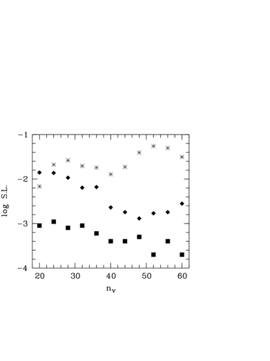
In order to detect and assess the significance of the alignments over the complete 3D sample, we used two statistical tests designed for circular data. The detailed procedure is described in Hutsemékers (1998). The basic idea is to compute for each quasar a statistics $S$ taking into account the compactness of a group of $n_{v}$ neighbors (in redshift space) and the dispersion of their polarization direction. The more compact and aligned a group of $n_{v}$ neighbors, the smaller the statistics $S$ . The second statistical test is the Andrew-Wasserman test designed by Bietenholz (1986). Both statistics can be calculated for the entire sample and the significance of a departure from homogeneity is assessed with Monte-Carlo reshuffling of the polarization direction over 3-D positions. The significance level is then computed as the probability that a random configuration has a smaller ( $S$ test) or higher statistics (Andrew-Wasserman test) than the observed one. Figure 3 Right frame shows the logarithm of the significance level of the Andrew-Wasserman test versus the number of neighbors $n_{v}$ for three samples of quasars. It clearly shows that, as the size of the sample increases, the alignments are harder and harder to produce from random distributions for any value of $n_{v}$ . Fig. 3 Left frame show the polarization map of the high redshift NGP sample (top) and the low redshift NGP sample (bottom). The length of the bars is proportional to $\sqrt{P}$ . Objects of both high and low polarization degrees participate to the same alignments. An unambiguous alignment effect of the polarization direction is visible at high redshift, whereas another alignment emerges at low redshift in a different direction.

Our statistical tests are not invariant under polar coordinates. A way to avoid coordinate dependence is to parallel transport the angles along great circle on the celestial sphere prior to computing the statistics. This was done by Jain et al. (2004). They confirm the significance of the alignments of the 213-quasar sample over very large regions of the NGP and SGP.

4. Discussion

The instrumental polarization can be discarded as a source of contamination because, it is very small on EFOSC2 ( $\sim$ 0.1%) and because the polarization degree and angle of quasars observed on different instruments are consistent within the errors. The contamination from the Galaxy is not a dominant component. Indeed, the interstellar polarization is usually much smaller than the polarization of quasars, and the interstellar polarization angles do not follow the quasar alignment directions. Moreover it is difficult to explain the redshift dependence of the alignment directions assuming a foreground interstellar screen. If we accept the fact that the alignments are intrinsic to the sources, we have to face correlated polarizations over extreme scales of Giga parsecs. Exotic sources of polarization on cosmological scales could be invoked, such as pervading exotic particles (Harari & Sikivie 1992; Jain et al. 2004) or an intrinsic alignment of the axes of quasar central engines. Future theoretical developments need to take these observed correlations into account.

The ongoing survey is paramount to characterize the alignments of quasar polarization directions accross the sky and correlate them with the other large-scale dataset (CMB, galaxy surveys, …). It will also allow us to deepen our knowledge of the linear polarization properties of quasars, and to understand the different source of linear polarization between the different species. We definitely need to increase the sample of polarized quasars from a few hundreds to a few thousands over the next decade to progress significantly in the field.

References

Berriman, G., Schmidt, G. D., West, S. C., & Stockman, H.S., ApJS, 1990, 74, 869.

Bietenholz M. F., 1986, AJ, 91, 1249.

Harari, D., & Sikivie, P. 1992, Phys. Lett. B, 289, 67

Heiles, C., 2000, AJ, 119, 923.

Hutsemékers, D., Sluse, D., Cabanac, R., Lamy, H., Quintana, H., in prep.

Sluse, D., Hutsemékers, D., Lamy, H., Cabanac, R., in prep.

Hutsemékers, D., 1998, A&A, 332, 410.

Hutsemékers, D., & Lamy, H., 2001, A&A, 367, 381.

Jain, P., Narain, G., & Sarala, S., MNRAS, 347, 394.

Lamy, H. & Hutsemékers, D., 1999, Msngr., 96, 25. (Erratum: The Messenger 97, 23)

Wardle, J. F. C. & Kronberg, P. P., 1974, ApJ, 194, 249.