Constraints on the Cardassian Expansion from the Cosmic Lens All-Sky Survey Gravitational Lens Statistics

Abstract

The existence of a dark energy component has usually been invoked as the most plausible way to explain the recent observational results. However, it is also well known that effects arising from new physics (e.g., extra dimensions) can mimic the gravitational effects of a dark energy through a modification of the Friedmann equation. In this paper we investigate some observational consequences of a flat, matter dominated and accelerating/decelerating scenario in which this modification is given by $H^{2}=g(\rho_{m},n,q)$ where $g(\rho_{m},n,q)$ is a new function of the energy density $\rho_{m}$, the so-called generalized Cardassian models. We mainly focus our attention on the constraints from the recent Cosmic All Sky Survey (CLASS) lensing sample on the parameters $n$ and $q$ that fully characterize the models. We show that, for a large interval of the $q-n$ parametric space, these models are in agreement with the current gravitational lenses data. The influence of these parameters on the acceleration redshift, i.e., the redshift at which the universe begins to accelerate, and on the age of the universe at high-redshift is also discussed.

1. Introduction

Over the last years, a considerable number of high quality observational data have transformed radically the field of cosmology. Results from distance measurements of type Ia supernovae (SNe Ia) (Perlmutter et al. 1999; Riess et al. 1998; 2004) combined with Cosmic Microwave Background (CMB) observations from ballon (de Bernardis et al. 2000; O’Dwyer et al. 2003), ground (Mason et al. 2003) and satelite experiments (Spergel et al. 2003) and with dynamical estimates of the quantity of matter in the universe (Calberg et al. 1996; Dekel et al. 1997) seem to indicate that the simple picture provided by the standard cold dark matter scenario (SCDM) is not enough. These observations are usually explained by introducing a new hypothetical energy component with negative pressure, the so-called dark energy or quintessence (For recent reviews on this topic, see Sahni & Starobinsky, 2000; Peebles & Ratra 2003; Padmanabhan, 2003; Lima, 2004 and references therein). Besides its consequences on fundamental physics, if confirmed, the existence of this dark component would also provide a definitive piece of information connecting the inflationary flatness prediction with astronomical data.

On the other hand, it is also well known that not less exotic mechanisms like, e.g., geometrical effects from extra dimensions may be capable of explaning such observational results. The basic idea behind these “braneworld cosmologies” is that our 4-dimensional Universe would be a surface or a brane embedded into a higher dimensional bulk space-time to which gravity could spread (Hořava & Witten, 1996a; 1996b; Randall L. & Sundrum, 1999; Dvali, Gabadadze & Porrati, 2000; Perivolaropoulos & Sourdis 2002; Maia et al., 2004). In some of these scenarios the observed acceleration of the Universe can be explained (without dark energy) from the fact that the bulk gravity sees its own curvature term on the brane acting as a negative-pressure dark component which accelerates the Universe. A natural conclusion from these and other similar studies is that dark energy, or rather, the gravitational effects of a dark energy could actually be achieved from a modification of the Friedmann equation arising from new physics.

Following this reasoning, several authors have recently investigated cosmologies with a modified Friedmann equation from extra dimensions as an alternative explanation for the recent observational data (Deffayet, Dvali & Gabadadze, 2002; Alcaniz, 2002; Jain, Dev & Alcaniz, 2002; Alcaniz, Jain & Dev, 2002; Lue & Starkman, 2003; Lue, Scoccimarro & Starkman, 2004; Alcaniz & Pires, 2004; Zhu & Alcaniz, 2004; Sahni & Shtanov 2004). For example, in Sahni & Shtanov (2002) a new class of braneworld models which admit a wider range of possibilities for dark energy than do the usual quintessence scenarios was investigated. For a subclass of the parameter values, the acceleration of the universe in this class of models can be a transient phenomena which could help reconcile an accelerating universe with the requirements of string/M-theory (Fischler et al. 2001).

Recently, Dvali & Turner (2003) explored the phenomenology and detectability of a correction on the Friedmann equation of the form $(1-\Omega_{m})H^{\alpha}/H_{o}^{\alpha-2}$, where $\Omega_{m}$ is the matter density parameter, $H$ is the Hubble parameter (the subscript “o” refers to present time) and $\alpha$ is a parameter to be adjusted by the observational data. Such a correction behaves like a dark energy with an effective equation of state given by $\omega=-1+\alpha/2$ in the recent past and like a cosmological constant ($\omega=-1$) in the distant future. Also based on extra dimensions physics, Freese & Lewis (2002) proposed the so-called Cardassian expansion, a model in which the universe is flat, matter dominated and currently accelerated. In the Cardassian universe, the new Friedmann equation is given by $H^{2}=g(\rho_{m})$, where $g(\rho_{m})$ is an arbitrary function of the matter energy density $\rho_{m}$. In the first version of these scenarios, the function $g(\rho_{m})$ was given by $g(\rho_{m})=A\rho_{m}+B\rho_{m}^{n}$, with the second term driving the acceleration of the universe at a late epoch after it becomes dominant (a detailed discussion for the origin of this Cardassian term from extra dimensions physics is given by Chung & Freese 2002. See also Cline & Vinet 2003). Although being completely different from the physical viewpoint, it was promptly realized that by identifying some free parameters Cardassian models and quintessence scenarios parameterized by an equation of state $p=\omega\rho$ predict the same observational effects in what concerns tests involving only the evolution of the Hubble parameter with redshift (Freese & Lewis 2002).

More recently, several forms for the function $g(\rho_{m})$ have been proposed (Freese 2003). In particular, Wang et al. (2003) have studied some observational characteristics of a direct generalization of the original Cardassian model. According to the authors, the observational expressions in this new scenario are very different from generic quintessence cosmologies and fully determined by two dimensionless parameters, $n$ and $q$. Observational constraints from a variety of astronomical data have also been investigated recently, both in the original Cardassian model (Zhu & Fujimoto 2002; 2003; Sen & Sen 2003a; 2003b) and in its generalized versions (Wang et al. 2003; Savage, Sugiyama & Freese 2004; Amarzguioui, Elgaroy & Multamaki, 2004). Perhaps the most interesting feature of Cardassian models is that although being matter dominated, they may be accelerating and may still reconcile the indications for a flat universe ($\Omega_{\rm{total}}=1$) from CMB observations with clustering estimates that point consistently to $\Omega_{m}\simeq 0.3$ with no need to invoke either a new dark component or a curvature term. In these scenarios, it happens through a redefinition of the value of the critical density (Freese & Lewis 2002) – see also below.

The aim of this paper is to test the viability of generalized Cardassian (GC) scenarios from statistical properties of gravitational lensing. To this end, we use the recent Cosmic All Sky Survey (CLASS) lensing sample, which constitutes the so far largest lensing sample suitable for statistical analysis. We show that for a large interval of the parameters $n$ and $q$ characterizing the models, GC scenarios are fully compatible with the current gravitational lensing observations. We also explore other observational aspects of the model like, e.g., those related to the acceleration redshift (i.e., the redshift at which the universe begins to accelerate) and to the age-redshift relation.

2. The generalized cardassian scenario

The modified Friedmann equation for GC models is (Wang et al. 2003)

$$H^{2}=\frac{8\pi G\rho_{m}}{3}\left[1+\left(\frac{\rho_{card}}{\rho_{m}}\right)^{q(1-n)}\right]^{1/q},$$ (1)

where $n$ and $q$ are two free parameters to be adjusted by the observational data, $\rho_{{card}}=\rho_{o}(1+z_{{card}})^{3}$ is the energy density at which the two terms inside the bracket become equal and $\rho_{o}$ is the present day matter density. Note that for values of $n=0$ and $q=1$, GC scenarios reduce to Cold Dark Matter models with a cosmological constant ($\Lambda$CDM). As explained in Wang et al. (2003), the first term inside the bracket dominates initially in such a way that the standard picture of the early universe is completely maintained. At a redshift $z_{{card}}$, these two terms become equal and, afterwards, the second term dominates, leading or not to an accelerated expansion (note, however, that $z_{card}$ is not necessarily the acceleration redshift. See, e.g., the discussion below on the deceleration parameter).

Evaluating Eq. (1) for present day quantities we find

$$H_{o}^{2}=\frac{8\pi G\rho_{o}}{3}\left[1+(1+z_{card})^{3q(1-n)}\right]^{1/q}.$$ (2)

From this equation, we see that $\rho_{o}$ is also the critical density that now can be written as

$$\rho_{o}=\rho_{c,old}\times\left[1+(1+z_{card})^{3q(1-n)}\right]^{-{1/q}},$$ (3)

where $\rho_{c,old}=1.88\times 10^{-29}h^{2}\rm{gm/cm^{3}}$ is the standard critical density and $h$ is the present day Hubble parameter in units of 100 ${\rm{km.s^{-1}Mpc^{-1}}}$. Note that for some combinations of the parameters $z_{card}$, $n$ and $q$ the critical density can be much lower than the one previously estimated. In other words it means that in the context of GC models it is possible to make the dynamical estimates of the quantity of matter that consistently point to $\rho_{o}\simeq(0.2-0.4)\rho_{c,old}$ compatible with the observational evidence for a flat universe from CMB observations and the inflationary flatness prediction with no need of a dark energy component (see Freese & Lewis (2002) for a more detailed discussion). In Fig. 1 we show a generalized version of the Figure 1 of Freese & Lewis (2002) in which the plane $z_{card}-n$ is displayed for selected values of $q$. The contours are labeled indicating the fraction of the standard critical density for different combinations of $z_{card}$ and $n$. In particular, the points inside the shadowed area delimited by the contours 0.2 - 0.4 are roughly consistent with the present clustering estimates (Calberg et al. 1996; Dekel et al. 1997).

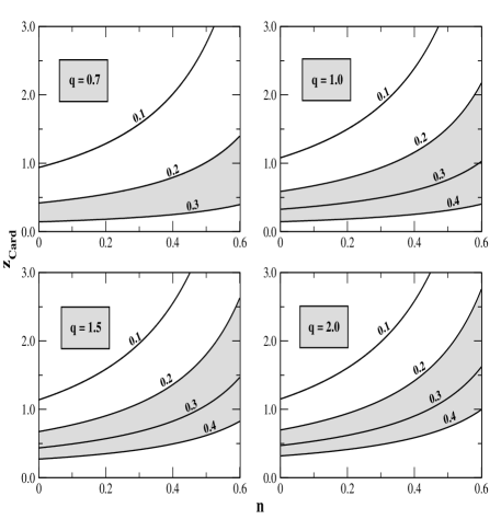
Figure 1.— $z_{card}-n$ diagrams for the ratio $\rho_{o}/\rho_{c,old}$ (Eq. 4) and selected values of $q$. The contours are labeled indicating the corresponding fraction of the standard critical density. Points inside the shadowed area are roughly consistent with the present clustering estimates (Calberg et al., 1996).

From Eq. (3), we see that the observed matter density parameter in GC models can be written as

$$\Omega_{m}^{obs}=\frac{\rho_{o}}{\rho_{c,old}}=\left[1+(1+z_{card})^{3q(1-n)}\right]^{-{1/q}}.$$ (4)

For the GC expansion parameterized by $n$ and $q$, the deceleration parameter as a function of the redshift has the following form

$$q(z)\equiv-\frac{\ddot{R}R}{\dot{R}^{2}}=-1+\frac{1}{2}\frac{d{\rm{ln}}f^{2}(z,\Omega_{m}^{obs},q,n)}{d{\rm{ln}}(1+z)},$$ (5)

where an overdot denotes derivative with respect to time, $R(t)$ is the cosmological scale factor and $f(z,\Omega_{m}^{obs},q,n)$ is given by Eq. (7). The behavior of the deceleration parameter as a function of redshift for some selected values of $n$ and $q$ and $\Omega_{m}^{obs}=0.3$ is shown in Figure 2. As discussed earlier, although completely dominated by matter, GC scenarios allow periods of accelerated expansion for some combinations of the parameters $n$ and $q$. Note that the present acceleration is basically determined by the value of $n$ and that the smaller its value the more accelerated is the present expansion for a given value of $q$. For example, for $q=1.5$ and $n=0$, GC models accelerate presently faster ($q_{o}\simeq-0.75$) than flat $\Lambda$CDM scenarios with $\Omega_{\Lambda}=0.7$ ($q_{o}\simeq-0.5$) although the acceleration redshift is almost identical ($z_{a}\simeq 0.7$) while for the same value of $q$ and $n=0.5$ we find $q_{o}\simeq-0.13$ and $z_{a}\simeq 0.52$. In order to make clear the difference between $z_{card}$ and $z_{a}$, for the latter values of $q$ and $n$, we find directly from Eq.(4) $z_{card}=1.06$. It means that although becoming dominant at $z_{card}\simeq 1$ the second term of Eq. (1) will drive an accelerated expansion only $\sim 1.7$ Gyr later, at $z_{a}\simeq 0.52$.

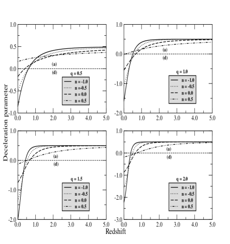
Figure 2.— Deceleration parameter as a function of redshift for some selected values of $n$ and $q$ and $\Omega_{m}^{obs}=0.3$. The horizontal line labeled (a)/(d) ($q_{o}=0$) divides models with a accelerating (a) or decelerating (d) expansion at a given redshift. As discussed in the text, the present value of $q_{o}$ is basically determined by the value of $n$.

From the above equations, it also is straightforward to show that the age-redshift relation is now given by (the total expanding age of the Universe $t_{o}$ is obtained by taking $z=0$)

$$t_{z}=\frac{1}{H_{o}}\int_{o}^{x^{\prime}}{dx\over xf(x,\Omega_{m}^{obs},q,n)},$$ (6)

where $x^{\prime}={R(t)\over R_{o}}=(1+z)^{-1}$ is a convenient integration variable and the dimensionless function $f(x,\Omega_{m}^{obs},q,n)$, obtained from Eqs. (1) and (4), is written as

$$f(x,\Omega_{m}^{obs},q,n)=\left\{\frac{\Omega_{m}^{obs}}{x^{3}}\left[1+\frac{(\Omega_{m}^{obs})^{-q}-1}{x^{-3q(1-n)}}\right]^{1/q}\right\}^{\frac{1}{2}}.$$ (7)

An interesting study on the total expanding age of the Universe in generalized Cardassian scenarios was recently presented by Savage et al. (2004). In light of first year WMAP data, it was shown that for a subset of Cardassian models the age of the universe varies in the interval 13.4 - 13.8 Gyr, which is surprisingly close to the standard $\Lambda$CDM prediction ($13.7\pm 0.2$ Gyr).

The angular diameter distance to a light source, defined as the ratio of the source diameter to its angular diameter, is an important concept in lensing statistics. For the class of GC models here investigated, the angular diameter distance, $D_{LS}(z_{L},z_{S})={R_{o}r_{1}(z_{L},z_{S})/(1+z_{S})}$, between two objects, for example a lens at $z_{L}$ and a source (galaxy) at $z_{S}$, reads

$$D_{LS}(z_{L},z_{S}) = \frac{H_{o}^{-1}}{(1+z_{S})}\int_{x^{\prime}_{S}}^{x^{\prime}_{L}}{dx\over x^{2}f(x,\Omega_{m}^{obs},q,n)}.$$ (8)

3. Lensing constraints using CLASS Sample

In this Section we present our study of statitical properties of gravitational lenses in GC scenarios based on the final CLASS well-defined statistical sample (for similar studies in quintessence and quartessence scenarios see, e.g., Chae et al. 2004; Jain et al. 2004).

The CLASS sample consists of 8958 radio sources out of which 13 sources are multiply imaged. Here we work only with those multiply imaged sources whose image-splittings are known (or likely) to be caused by single galaxies. There are 9 such radio sources: 0218+357, 0445+123, 0631+519, 0712+472, 0850+054, 1152+199, 1422+231, 1933+503, 2319+051. We, therefore, following Chae et al. (2002) and Dev, Jain & Mahajan (2004), work with a total of 8954 radio source. The sources probed by CLASS at $\nu=5$ GHz are well represented by power-law differential number-flux density relation: $\left|dN/dS\right|\propto(S/S^{0})^{\eta}$ with $\eta=2.07\pm 0.02$ ($1.97\pm 0.14$) for $S\geq S^{0}$ ($\leq S^{0}$) where $S^{0}=30$ mJy (Browne et al., 2003). The CLASS unlensed sources can be adequately described by a Gaussian model with mean redshift $z=1.27$ and a dispersion of $0.95$.

In our analysis we assume the singular isothermal sphere (SIS) model for the lens mass distribution (Turner, Ostriker & Gott 1984). For the present analysis we also ignore the evolution of the number density of galaxies and assume that the comoving number density is conserved and currently given by

$$n_{o}=\int_{0}^{\infty}\phi(L)dL,$$ (9)

where $\phi(L)$ is the well known Schechter Luminosity Function (LF). The differential optical depth of lensing in traversing $dz_{L}$ with angular separation between $\phi$ and $\phi+d\phi$ is (Fukugita, Futamase & Kasai, 1990, Turner, 1990; Fukugita et al., 1992)

$$\frac{d^{2}\tau}{dz_{L}d\phi}d\phi dz_{L} = F^{*}\,(1+z_{L})^{3}\,\left({{D_{OL}D_{LS}}\over{R_{o}D_{OS}}}\right)^{2}\ \frac{1}{R_{o}}\,\frac{cdt}{dz_{L}}\times$$ (10)

$$\times\frac{\gamma/2}{\Gamma(\alpha+1+\frac{4}{\gamma})}\left(\frac{D_{OS}}{D_{LS}}\phi\right)^{\frac{\gamma}{2}(\alpha+1+\frac{4}{\gamma})}$$

$$\times{\rm{exp}}\left[-\left(\frac{D_{OS}}{D_{LS}}\phi\right)^{\frac{\gamma}{2}}\right]\frac{d\phi}{\phi}dz_{L},$$

where the function $F^{*}$ is defined as

$$F^{*}={16\pi^{3}\over{c\,H_{0}^{3}}}\phi_{\ast}v_{\ast}^{4}\Gamma\left(\alpha+{4\over\gamma}+1\right).$$ (11)

In Eq. (10) $D_{OL}$, $D_{OS}$ and $D_{LS}$ are, respectively, the angular diameter distances from the observer to the lens, from the observer to the source and between the lens and the source (see Eq. 8). In order to relate the characteristic luminosity $L_{*}$ to the characteristic velocity dispersion $v_{*}$, we use the Faber-Jackson relation (Faber & Jackson, 1976) for early-type galaxies ($L_{*}\propto{v_{*}}^{\gamma}$), with $\gamma=4$. For the analysis presented here we neglect the contribution of spirals as lenses because their velocity dispersion is small when compared to ellipticals.

Two large-scale galaxy surveys, namely, the 2dF Galaxy Redshift-Survey (2dFGRS) and the Sloan Digital Sky Survey (SDSS) have produced converging results on the total LF. These surveys determined the Schechter parameters for galaxies (all types) at $z\leq 0.2$. For our analysis here, we adopt the normalization corrected Schechter parameters of the 2dFGRS survey (Folkes et al. 1999; Chae 2002): $\alpha=-0.74$, $\phi^{*}=0.82\times 10^{-2}h^{3}\mathrm{Mpc^{-3}}$, $v^{*}=185\,\mathrm{km/s}$ and $F^{*}=0.014$.

The total optical depth $\tau(z)$ along the line of sight from an observer at $z=0$ to a source at $z_{S}$ is given by

$$\tau(z_{S})=\frac{F^{*}}{30}\left[D_{OS}(1+z_{S})\right]^{3}R_{o}^{3}.$$ (12)

where $D_{OS}$ is given by Eq. (8). Figure 3 shows, for the fixed value of $\Omega_{m}^{obs}=0.3$, the normalized optical depth as a function of the source redshift for values of $q=$ 0.3, 1.0, 2.0 and 3.0 and $n=$ -1.0, -0.5, 0.0 and 0.5. Note that a decrease in the value of $n$ at fixed $\Omega_{m}^{obs}$ and $q$ tends to increase the optical depth for lensing. For $q=1.0$ at $z_{S}=3.0$, the value of $\tau/F^{*}$ for $n=0.5$ is down from that one for $n=-1.0$ by a factor of $\sim 2.02$, while the same values of $n$ and $q=2.0$ provide values for $\tau/F^{*}$ that are up from the previous ones only by a factor of $\sim$ 1.1 and 1.25, respectively. It clearly shows that the optical depth is a more sensitive function to the parameter $n$ than to the index $q$. As commented earlier, this particular feature is also noted for the other analyses discussed in this paper.

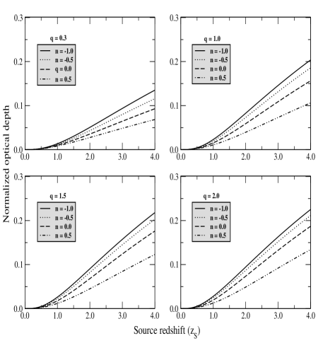
Figure 3.— Normalized optical depth ($\tau/F^{*}$) as a function of the source redshift $z_{S}$ for some selected valuesof $n$ and $q$ and a fixed value of $\Omega_{m}^{obs}=0.3$.

The normalized image angular separation distribution for a source at $z_{S}$ is obtained by integrating $\frac{d^{2}\tau}{dz_{L}\,d\phi}$ over $z_{L}$, i.e.,

$${d{\mathcal{P}}\over d\phi}\,=\,{1\over\tau(z_{S})}\int_{0}^{z_{s}}\,{\frac{d^{2}\tau}{dz_{L}d\phi}}{dz_{L}}.$$ (13)

The corrected (for magnification and selection effects) image separation distribution function for a single source at redshift $z_{S}$ is given by (Kochanek, 1996; Chiba & Yoshii, 2001)

$$P^{\prime}(\Delta\theta)\, = \,\mathcal{B}\,{{{\gamma}}\over 2\,\Delta\theta}\int_{0}^{z_{S}}\left[{D_{OS}\over{D_{LS}}}\phi\right]^{{\frac{\gamma}{2}}(\alpha+1+{\frac{4}{\gamma}})}\,F^{*}\,{cdt\over dz_{L}}\times$$ (14)

$$\times\exp\left[-\,\left({D_{OS}\over{D_{LS}}}\phi\right)^{\frac{\gamma}{2}}\right]{(1+z_{L})^{3}\over\Gamma\left(\alpha+{4\over\gamma}+1\right)}$$

$$\times\left[\,\left({D_{OL}D_{LS}\over R_{0}D_{OS}}\right)^{2}\,{1\over R_{0}}\right]\,\,{dz_{L}}.$$

Similarly, the corrected lensing probability for a given source at redshift $z$ can be written as

$$P^{\prime}=\tau(z_{S})\,\int{d{\mathcal{P}}\over d\phi}\mathcal{B}\;d\phi,$$ (15)

where $\phi$ and $\Delta\theta$ are related to as $\phi={\frac{\Delta\theta}{8\pi(v^{*}/c)^{2}}}$ and $\mathcal{B}$ is the magnification bias. It is worth emphasizing that this is considered because, as widely known, gravitational lensing causes a magnification of images and this transfers the lensed sources to higher flux density bins. In other words, the lensed sources are over-represented in a flux-limited sample.

The magnification bias ${\mathcal{B}}(z_{S},S_{\nu})$ increases the lensing probability significantly in a bin of total flux density ($S_{\nu}$) by a factor

$$\mathcal{B}(z_{S},S_{\nu})\, = \,\left|\frac{dN_{z_{S}}(>S_{\nu})}{dS_{\nu}}\right|^{-1}$$

$$\times\int_{\mu_{min}}^{\mu_{max}}\left|\frac{dN_{z_{S}}(>S_{\nu}/\mu)}{dS_{\nu}}\,p(\mu)\right|{1\over\mu}\,d\mu.$$

Here $N_{z_{S}}(>S_{\nu})$ is the intrinsic flux density relation for the source population at redshift $z_{S}$. $N_{z_{S}}(>S_{\nu})$ gives the number of sources at redshift $z_{S}$ having flux greater than $S_{\nu}$. For the SIS model, the magnification probability distribution is $p(\mu)=8/{\mu}^{3}$. The minimum ($\mu_{min}$) and maximum ($\mu_{max}$) total magnifications in Eq. (16) depend on the observational characteristics as well as on the lens model. For the SIS model, the minimum total magnification is $\mu_{min}\simeq 2$ while $\mu_{max}=\infty$. The magnification bias $\mathcal{B}$ depends on the differential number-flux density relation $\left|dN_{z_{S}}(>S_{\nu})/dS_{\nu}\right|$, which means that such a relation needs to be known as a function of the source redshift. Since, at present, redshifts of only a few CLASS sources are known, we ignore redshift dependence of the differential number-flux density relation. Following Chae (2002), we further ignore the dependence of the differential number-flux density relation on the spectral index of the source.

Finally, we emphasize that two important selection criteria for CLASS statistical sample are (i) that the ratio of the flux densities of the fainter to the brighter images ${\mathcal{R}}_{min}$ is $\geq 0.1$. Given such an observational limit, the minimum total magnification for double imaging for the adopted model of the lens is $\mu_{min}=2(1+\mathcal{R}_{min}/1-\mathcal{R}_{min})$; (ii) that the image components in lens systems must have separations $\geq 0.3$   arcsec. We incorporate this selection criterion by setting the lower limit of $\Delta\theta$ in equation (15) as $0.3$ arcsec.

We perform a maximum-likelihood analysis to determine the confidence levels in the $n-q$ space. The likelihood function is defined by

$${\cal{L}}=\prod_{i=1}^{N_{U}}(1-P^{{}^{\prime}}_{i})\,\prod_{k=1}^{N_{L}}P^{\prime}(\Delta\theta),$$ (17)

where $N_{L}$ is the observed number of multiple-imaged lensed radio sources and $N_{U}$ is the number of unlensed sources in the adopted sample. $P_{i}^{{}^{\prime}}$ is the probability of the $i^{th}$ source to get lensed and $P_{k}^{{}^{\prime}}(\Delta\theta)$ is the probability of the $k^{th}$ source to get lensed with the observed image separation $\Delta\theta$.

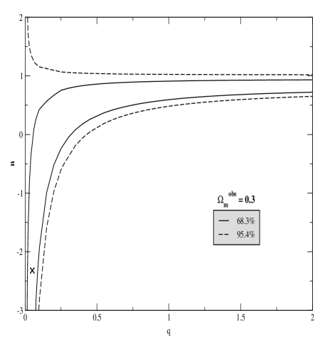
Figure 4.— Confidence regions in the plane $n-q$ arising from lensing statistics for a fixed value of $\Omega_{m}^{obs}=0.3$. Solid (dashed) lines indicate contours of constant likelihood at $68.3\%$ c.l. ($95.4\%$ c.l.). The best-fit model is indicated by “$\times$”.

Figure 4 shows the main results of our analysis. There, we show contours of constant likelihood ($68.3\%$ and $95.4\%$) in the parameter space $n-q$. From the above equation we find that the maximum value of the likelihood function is located at $n=-2.32$ and $q=0.05$, which means that the cardassian term of Eq. (1) takes over only recently, i.e., at $z_{card}\simeq{\cal{O}}(10^{-3})$. At the 1$\sigma$ level, however, the entire range of $q$ (if we consider for instance $0<q\leq 2$) is compatible with the observational data for a fixed value of $\Omega_{m}^{obs}=0.3$ (a similar conclusion also holds for small variations on the value of $\Omega_{m}^{obs}=0.3$, i.e., $\pm 0.1$, which is inside the uncertainties of current clustering estimates). As observed earlier, this result suggests that a large class of GCs cenarios is in accordance with the current gravitational lensing data. This best-fit scenario also corresponds to a $7.7h^{-1}$-Gyr-old universe ($z=0$) and provides an universe old enough to accommodate some recent age estimates of high-$z$ objects. For example, at $z=1.55$ and $z=1.43$ Eq. (6) provides $t_{z}\simeq 3.5$ Gyr and $t_{z}\simeq 3.7$ Gyr, respectively, i.e., values that are in agreement with the age estimates for the radio galaxies LBDS 53W091 and LBDS 53W069 (Dunlop et al. 1996; Dunlop 1988; Alcaniz & Lima 1999). For the recent discovery of the quasar APM 08279+5255 (Hasinger & Komossa 2002; Komossa & Hasinger 2003) at $z=3.91$, however, these values of $q$ and $n$ provide $t_{z}\simeq 1.4$ Gyr while the age estimate for this object lies between 2.0 - 3.0 Gyr. A similar problem is also faced by several cosmological scenarios, including the current concordance $\Lambda$CDM model (see Friaça, Alcaniz & Lima, 2004).

4. Conclusion

The possibility of an accelerating universe from distance measurements of type Ia supernovae constitutes one of the most important results of modern cosmology. These observations naturally lead to the idea of a dominant dark energy component with negative pressure since all known types of matter with positive pressure generate attractive forces and decelerate the expansion of the universe [$\ddot{R}\propto-(\rho+3p$)]. On the other hand, the realization that dark energy or the effects of dark energy could be a manifestation of a modification to the Friedmann equation arising from extra dimension physics has opened up an unprecedented opportunity to establish a more solid connection between particle physics and cosmology. Many braneworld scenarios have been proposed in the recent literature with some of them presenting interesting features which make them a natural alternative to the standard model. Here we have analyzed some observational consequences of one of these scenarios, the so-called generalized cardassian expansion, recently proposed by Wang et al. (2003). We have studied the observational constraints on the parameters $n$ and $q$ that fully characterize the model from statistical properties of gravitational lensing. To this end, we have used the final CLASS well-defined statistical sample, which constitutes the most recent gravitational lensing data. From our analysis we have found that at $1\sigma$ level a large portion of the parametric space $q-n$ is in agreement with the current gravitational lensing observations, with the maximum of the likelihood function located at $n=-2.32$ and $q=0.05$ which corresponds to a $7.7h^{-1}$-Gyr-old universe and $z_{card}\simeq{\cal{O}}(10^{-3})$. These and other similar results show that there exist viable and interesting alternatives to our current standard cosmological model ($\Lambda$CDM) based on extra dimension physics. Further observational analysis on the generalized cardassian scenario will appear in a forthcoming communication.

References

- (1) Alcaniz J. S., 2002, Phys. Rev. D65, 123514. astro-ph/0202492
- (2) Alcaniz J. S., Jain D. and Dev A., 2002, Phys. Rev. D66, 067301. astro-ph/0206448
- (3) Alcaniz J. S. and Lima J. A. S., 1999, ApJ, 521, L87. astro-ph/9902298
- (4) Alcaniz J. S. and Pires N., 2004, Phys. Rev. D70, 047303. astro-ph/0404146
- (5) Alcaniz J.S. and Zhu Z.-H. 2004. astro-ph/0411604
- (6) Amarzguioui M., Elgaroy O. and Multamaki T., 2004.astro-ph/0410408
- (7) Browne I. W. A. et al., 2003, Mon. Not. Roy. Astron. Soc. 341, 13
- (8) Calberg R. G. et al., 1996, ApJ, 462, 32
- (9) Chae K. -H., 2002. astro-ph/0211244
- (10) Chae K. -H. et al., 2002, Phys. Rev. Lett., 89,
- (11) Chae K. -H., Chen G., Ratra B. and Lee D-W, 2004, ApJ, 607, L71 151301
- (12) Chiba M. and Yoshii Y., 2001, ApJ, 510, 42
- (13) Chung D. J. and Freese K., 2002, Phys. Rev. D61, 023511
- (14) Cline J. M. and Vinet J., 2003, Phys. Rev. D68 025015
- (15) de Bernardis P. et al., 2000, Nature, 404, 955
- (16) Dekel A., Burstein D. and White S., In Critical Dialogues in Cosmology, edited by N. Turok World Scientific, Singapore (1997)
- (17) Deffayet C., 2001, Phys. Lett. B 502, 199
- (18) Deffayet C., Dvali G. and Gabadadze G., 2002, Phys. Rev. D65, 044023
- (19) Dev A., Jain D. and Mahajan S., 2004, Int. J. Mod. Phys. D13, 1005
- (20) Dunlop J. et al., 1996, Nature, 381, 581
- (21) Dunlop J., in The Most Distant Radio Galaxies, ed. H. J. A. Rottgering, P. Best, & M. D.Lehnert, Dordrecht: Kluwer, 71 (1999)
- (22) Dvali G., Gabadadze G. and Porrati M., 2000, Phys. Lett. B485, 208
- (23) Dvali G. and Turner M. S., 2003. astro-ph/0301510
- (24) Faber S. M. and Jackson R. E., 1976, ApJ, 204, 668
- (25) Folkes S. et al., 1999, Mon. Not. Roy. Astron. Soc., 308, 459
- (26) Fischler W., Kashani-Poor A., McNees R. and Paban S., 2001, JHEP, 0107, 003
- (27) Freedman W. L. et al., 2001, ApJ, 553, 47
- (28) Freese K., 2003, Nuc. Phys. B (Proc. Suppl.) 124, 50
- (29) Freese K. and Lewis M., 2002, Phys. Lett. B540, 1
- (30) Friaça A. S. C., Alcaniz J. S. & Lima J. A. S., Submited to MNRAS. 2004
- (31) Fukugita M., Futamase T. and Kasai M., 1990, MNRAS, 246, 24
- (32) Fukugita M., Futamase T., Kasai M. and Turner E.L., 1992, ApJ, 393, 3
- (33) Hasinger G., Schartel N. and Komossa S., 2002, ApJ, 573, L77
- (34) Hořava P. and Witten E., 1996, Nucl. Phys. B460, 606; 1996, Nucl. Phys. B475, 94
- (35) Jain D., Dev A. and Alcaniz J. S., 2002, Phys. Rev. D66, 083511. astro-ph/0206224
- (36) Jain D., Alcaniz J. S. and Dev. A., 2004. astro-ph/0409431
- (37) Kochanek C. S., 1996, ApJ, 466, 638
- (38) Komossa S. and Hasinger G., in XEUS studying the evolution of the universe, G. Hasinger et al. (eds), MPE Report 281, 285 (2003).
- (39) Lima J. A. S., 2004, Braz. J. Phys. 34, 194
- (40) Lue A. and Starkman G. D., 2003, Phys. Rev. D67, 064002
- (41) Lue A., Scoccimarro R. and Starkman G. D., 2004 astro-ph/0401515
- (42) Maia M. D. et al., 2004, astro-ph/0403072
- (43) Mason, B. S. et al. 2003, ApJ, 591, 540
- (44) Multamaki T., Gaztanaga E. and Manera M., 2003. Submitted to MNRAS. astro-ph/0303526
- (45) O’Dwyer I. J. et al. 2003. astro-ph/0312610
- (46) Padmanabhan T., 2003, Phys. Rept. 380, 235
- (47) Peebles P. J. E. and Ratra B., 2003, Rev. Mod. Phys. 75, 559
- (48) Perivolaropoulos L. and Sourdis C., 2002, Phys. Rev. D66, 084018
- (49) Perlmutter S. et al., 1999, ApJ 517, 565
- (50) Randall L., 2002, Science, 296, 1422
- (51) Randall L. and Sundrum R., 1999, Phys. Rev. Lett. 83, 3370
- (52) Riess A. G. et al., 1998, AJ116, 1009
- (53) Riess A. G. et al., 2004, ApJ, 607, 665
- (54) Sahni V. and Shtanov Y., 2002, Int. J. Mod. Phys., 11, 1
- (55) Sahni V. and Starobinsky A., 2000, Int. J. Mod. Phys. D9, 373
- (56) Sahni V. and Shtanov Y., 2004. astro-ph/0410221
- (57) Sen S. and Sen A. A., 2002. astro-ph/0211634
- (58) Sen A. A. and Sen S., 2003. astro-ph/0303383
- (59) Spergel D. N. et al., 2003, ApJ Suppl. 148, 17
- (60) Turner E. L., 1990, ApJ, 365, L43
- (61) Turner E. L., Ostriker J. P. and Gott J. R., 1984, ApJ, 284, 1
- (62) Wang Y., Freese K., Gondolo P. and Lewis M., 2003, ApJ, 594, 25
- (63) Zhu Z.-H. and Alcaniz J. S., ApJ (in press). astro-ph/0404201
- (64) Zhu Z.-H. and Fujimoto M.-K., 2002, ApJ, 581, 1
- (65) Zhu Z.-H. and Fujimoto M.-K., 2003, ApJ, 585, 52