The far-infrared emission line and continuum spectrum of the Seyfert galaxy NGC 1068

Abstract

We report on the analysis of the first complete far-infrared spectrum (43-197$\mu$m) of the Seyfert 2 galaxy NGC 1068 as observed with the Long Wavelength Spectrometer (LWS) onboard the Infrared Space Observatory (ISO). In addition to the 7 expected ionic fine structure emission lines, the OH rotational lines at 79, 119 and 163$\mu$m were all detected in emission, which is unique among galaxies with full LWS spectra, where the 119$\mu$m line, when detected, is always in absorption. The observed line intensities were modelled together with ISO Short Wavelength Spectrometer (SWS) and optical and ultraviolet line intensities from the literature, considering two independent emission components: the AGN component and the starburst component in the circumnuclear ring of $\sim$ 3 kpc in size. Using the UV to mid-IR emission line spectrum to constrain the nuclear ionizing continuum, we have confirmed previous results: a canonical power-law ionizing spectrum is a poorer fit than one with a deep absorption trough, while the presence of a big blue bump is ruled out. Based on the instantaneous starburst age of 5 Myr constrained by the Br $\gamma$ equivalent width in the starburst ring, and starburst synthesis models of the mid- and far-infrared fine-structure line emission, a low ionization parameter (U=10^-3.5) and low densities (n=100 cm^-3) are derived. Combining the AGN and starburst components, we succeeded in modeling the overall UV to far-IR atomic spectrum of NGC 1068, reproducing the line fluxes to within a factor 2.0 on average with a standard deviation of 1.3, and the overall continuum as the sum of the contribution of the thermal dust emission in the ionized and neutral components. The OH 119 $\mu$m emission indicates that the line is collisionally excited, and arises in a warm and dense region. The OH emission has been modeled using spherically symmetric, non-local, non-LTE radiative transfer models. The models indicate that the bulk of the emission arises from the nuclear region, although some extended contribution from the starburst is not ruled out. The OH abundance in the nuclear region is expected to be $\sim 10^{-5}$, characteristic of X-ray dominated regions.

1. INTRODUCTION

NGC 1068 is known as the archetypical Seyfert type 2 galaxy. It is nearby, luminous (${\rm L_{IR}=2\times 10^{11}L_{\odot}}$ Bland-Hawthorn et al., 1997), and it has been extensively observed and studied in detail from X-rays to radio wavelengths. With a measured redshift of z=0.0038 (Huchra et al., 1999) (corresponding to a distance of D=15.2 Mpc for H₀=75 km s^-1 Mpc^-1), it provides a scale of only $\sim$ 74 pc/$\arcsec$. A central nuclear star cluster has an extent of $\sim$ 0.6$\arcsec$ (Thatte et al., 1997) and a 2.3 kpc stellar bar observed in the near-IR (Scoville et al., 1988; Thronson et al., 1989) is surrounded by a circumnuclear starburst ring. Telesco et al. (1984) found that the infrared emission in NGC 1068 was due to both the Seyfert nucleus (which dominates the 10$\mu$m emission) and to the star forming regions in the bright $\sim$ 3kpc circumnuclear ring (which emits most of the luminosity at $\lambda>30{\mu}m$). A $Br\gamma$ imaging study (Davies, Sugai & Ward, 1998) showed a similar morphology and indicated that a short burst of star formation occurred throughout the circumnuclear ring of 15-16^′′ in radius within the last 4-40 Myr. CO interferometer observations revealed molecular gas very close to the nucleus ($\sim$0.2$\arcsec$) suggesting the presence of $\sim$ 10${}^{8}M_{\sun}$ within the central 25pc (Schinnerer et al., 2000). Recent high resolution H₂ line emission mapping indicates the presence of two main nuclear emission knots with a velocity difference of 140 km/s, which, if interpreted as quasi-keplerian, would imply a central enclosed mass of 10${}^{8}M_{\sun}$ (Alloin et al., 2001).

In this article, we present the first complete far-infrared spectrum from 43 to 197$\mu$m showing both atomic and molecular emission lines (§2). We model the composite UV- to far-IR atomic emission line and continuum spectrum, from our data and the literature, using photoionization models of both the active nucleus and the starburst component (§3). We also model the mid- to far-IR continuum emission using a radiative transfer code and gray body functions for the neutral molecular components (§4). Moreover, two different non-local, non-LTE radiative transfer codes have been used to model the OH lines (§5). Our conclusions are then given in §6.

2. OBSERVATIONS

NGC 1068 was observed with the Long Wavelength Spectrometer (LWS) (Clegg et al., 1996) on board the Infrared Space Observatory (ISO) (Kessler et al., 1996), as part of the Guaranteed Time Programme of the LWS instrument team. The full low resolution spectrum (43-197$\mu$m) of NGC 1068 was collected during orbit 605 (July 13, 1997). Two on-source full scans (15,730 seconds of total integration time) and two off-source (6’ N) scans of the [CII]158$\mu$m line (3,390 seconds of total integration time) were obtained. On- and off-source scans had the same integration time per spectral step. Because of the design of the LWS spectrometer, simultaneously with the 158$\mu$m data, a short spectral scan of equal sensitivity to the on-source spectrum was obtained at sparsely spaced wavelengths across the LWS range.

The LWS beam is roughly independent of wavelength and equal to about 80 arcsec. The spectra were calibrated using Uranus, resulting in an absolute accuracy better than 30% (Swinyard et al., 1996). The data analysis has been done with ISAP, starting from the auto-analysis results processed through the LWS Version 7-8 pipeline (July 1998). To be confident that newer versions of the pipeline and calibration files did not yield different results, we have compared our data with the results obtained using pipeline 10.1 (November 2001) and we did not find significant differences in the line fluxes or the continuum.

All the full grating scans taken on the on-source position and the two sets of data on the off-source position were separately co-added. No signal was detected in the off-source coadds. The emission line fluxes were measured with ISAP, which fits polynomials to the local continuum and Gaussian profiles to the lines. In all cases the observed line widths were consistent with the instrumental resolution of the grating, which was typically 1500 km/sec. The integrated line fluxes measured independently from data taken in the two scan directions agreed very well, to within 10%. The on source LWS spectrum that resulted from stitching the ten LWS channels together using small multiplicative corrections in order to match the overlapping regions of each channel with its neighbors is shown in Fig. 1. LWS spectra of sources that are very extended within the instrument beam or that peak off center are typically affected by channel fringing in the continuum baseline (Swinyard et al., 1998). Fortunately, these spurious ripples are hardly noticeable in our LWS spectrum, presumably because the far-IR continuum is centrally concentrated towards the center of the LWS $80^{\prime\prime}$ beam.

Besides the LWS observations, we also use the SWS observations presented by Lutz et al. (2000), to extend the wavelength and ionization-level coverage. Table 1 presents all the ISO line flux measurements including those from the SWS with their respective aperture sizes.

3. THE FINE STRUCTURE LINES

To be able to better constrain the modeling of the line emission of NGC 1068, we have combined our far-infrared fine structure line measurements (Table 1) with ultraviolet, optical and infrared spectroscopic data from the literature (Kriss et al., 1992; Marconi et al., 1996; Thompson, 1996; Lutz et al., 2000). The complete emission line spectrum of NGC 1068 from the ultraviolet to the far-IR includes several low-ionization lines that are primarily produced outside the narrow line region (NLR) of the active nucleus, as well as intermediate ionization lines that originate from both starburst and AGN emission. For this reason, we find that no single model satisfactorily explains all the observed emission lines. We identify two main components:

• an AGN component (the NLR), exciting the high ionization lines and contributing little to the low-to-intermediate ionization lines;

• a starburst component in the circumnuclear ring of the galaxy (e.g. Davies, Sugai & Ward, 1998) that produces the low ionization and neutral forbidden lines and some of the emission in the intermediate ionization lines. This component should also produce emission associated with photo-dissociation regions (PDRs) (e.g. Kaufman et al., 1999), at the interface with the interstellar medium of the galaxy.

In this section, we will examine separately the two components that produce the total fine structure emission line spectrum of NGC 1068, namely the AGN and the starburst, for which we propose two different computations, and we add together these components to reproduce the overall observed spectrum from the UV to the far-IR in §3.3.

3.1. Modeling the AGN

The first photoionzation model predictions of the mid to far-infrared emission line spectra of the Narrow Line Regions (NLR) of active galaxies were presented by Spinoglio & Malkan (1992), well before the ISO observations could be collected. Alexander et al. (2000) used the observed high ionization emission lines to model the obscured ionizing AGN continuum of NGC 1068 and found that the best-fit spectral energy distribution (SED) has a deep trough at 4 Rydbergs, which is consistent with an intrinsic “big blue bump” that is partially obscured by $\sim$ $6\times 10^{19}$ cm^-2 of neutral hydrogen interior to the NLR. Following their results, we have simulated their models, although using a different photoionization code, CLOUDY (Version 96, Ferland et al., 1998; Ferland, 2000), and then we have varied the shape of the ionizing continuum to include the ionizing continuum derived in Pier et al. (1994). Our goal was to test if the Alexander et al. (2000) results were unique and to fit the remaining emission by a starburst component, and thereby to derive a composite model of the complete emission line spectrum of NGC 1068.

Specifically, we explore three plausible AGN SEDs. Model A assumes the best fit ionizing spectrum derived by Alexander et al. (2000), i.e. with a deep trough at 4 Rydberg (log$f$ = -27.4, -29.0, -27.4, -28.2 at 2, 4, 8 and 16 Ryd, respectively). An intrinsic nuclear spectrum of NGC 1068 has also been inferred by Pier et al. (1994). Model B assumes the original ionizing spectrum derived from Pier et al. (1994). Model C assumes an SED with a Big Blue Bump superposed on the Pier et al. (1994) ionizing continuum (log$f$ = -25.8, -25.8, -25.8, -27.4 at 2, 4, 8 and 16 Ryd, respectively) as expected for the thermal emission of an accretion disk around a central black hole. These three AGN ionizing continua are plotted in Fig. 1. For each of models A, B, and C, we have used two component models with the same parameters as in Alexander et al. (2000): component 1 has a constant hydrogen density of 10⁴cm^-3, an ionization parameter U=0.1, a covering factor c=0.45, a filling factor of 6.5 $\times$ 10^-3 with a radial dependence of the form r^-2, and extends from $\sim$ 21 to $\sim$ 109 pc from the center; component 2 has a density of 2 $\times$ 10³ cm^-3, an ionization parameter U=0.01, a covering factor of c=0.29, a filling factor of 6.5 $\times$ 10^-4 without any radial dependence, and extends from $\sim$ 153 to $\sim$ 362 pc from the center. We have also assumed the “low oxygen” abundances adopted by Alexander et al. (2000), in order to be able to compare our results with theirs. Because the grain physics has been updated in the most recent version of CLOUDY (Version 96), we have included the presence of grains in the models, using “Orion-type” grains. The inclusion of grains also allows us to compute the thermal dust continuum emission from the ionized components (see §4).

The inner and outer radii of the emission regions of the two components, 21, 109, 153 and 362 pc, correspond to angular distances of about 0.26, 1.4, 1.9 and 4.5 $\arcsec$, respectively. Table 2 reports the predicted line fluxes of the three AGN models, A, B, and C, together with the observed line fluxes: the line fluxes are given for each of the two components 1 and 2, which are treated as independent, and the total flux for each model is simply the sum of the fluxes of the two components.

We can see from Table 2 that only the AGN A and B models, and not the AGN C model, reproduce most of the observed high ionization line fluxes. The low and intermediate ionization lines, are expected to have partial or full contributions from starburst and PDR components (see §3.2). This first result rules out the presence of a “big blue bump” in the ionizing continuum of NGC 1068. To be able to compare the modeled ultraviolet and optical lines with the observations, we also listed in Table 2 and  3 their dereddened fluxes, assuming two values for the extinction: E_B-V = 0.4 mag (Malkan & Oke, 1983) and E_B-V = 0.2 mag (Marconi et al., 1996). We find that the AGN B model overpredicts several of the intermediate ionization lines, such as [SIV]10.5$\mu$m, [NeIII]15.6$\mu$m and [SIII]18.7$\mu$m, and this discrepancy increases when adding the starburst component because these lines are also copiously produced by that component (see next section). On the other hand, the [NeII]12.8$\mu$m emission is underpredicted so much so that even with the inclusion of the starburst component it cannot be reproduced with this model. As we discuss further in §3.3, a composite AGN/starburst model using AGN model A reproduces the [NeII]12.8$\mu$m emission better than the other composite models.

3.2. Modeling the starburst ring

NGC 1068 is known to emit strong starburst emission from the ring-like structure at a radial distance of $15-16^{\prime\prime}$ from the nucleus (total size of $\sim$ 3 kpc), traced for example by the Br $\gamma$ emission (Davies, Sugai & Ward, 1998). Mid-IR line imaging observations of NGC 1068 have been published by Le Floc’h et al. (2001) based on ISOCAM CVF observations. They presented an image of the 7.7 $\mu$m PAH feature that shows constant surface brightness above the 4th coutour near the nucleus. This suggests that star formation is occuring in the direction of the nucleus so that nuclear spectra will include some emission from star formation. In the case of the SWS observations that we are modeling (reported by Lutz et al. (2000)), three apertures were used at different wavelengths with the two largest also including portions of the brighter starburst ring (see Table 1). To estimate how much of the starburst emission is contained in the different apertures used in the observations, we have used a continuum subtracted image in the 6.2 $\mu$m feature produced by C. Dudley (private communication) using the same ISOCAM CVF data set examined by Le Floc’h et al. (2001). The 6.2 $\mu$m feature is more isolated than the 7.7 $\mu$m feature, which is blended with the 8.7 $\mu$m feature and the silicate absorption feature, but the image compares well with the published 7.7 $\mu$m image though we have zeroed out the residuals in a 3$\times$12 arcsec² region centered on the nucleus. Based on this image, the SWS 14$\times$20, 14$\times$27 and 20$\times$33 arcsec² slits contain 13, 23 and 46% of the 6.2 $\mu$m flux contained in the LWS beam respectively, without correction for the neglected region of poor residuals (oriented at 45^∘ to our synthetic SWS slits). Since PAH features are thought to be a good tracer of PDRs and their associated startbursts, we adopt these percentages in our model predictions of SWS line strengths in the starburst models presented in this section. In fitting our starburst models to the observations, we have computed the line fluxes at earth of each centrally illuminated emitting cloud and then determined the number of clouds needed to best fit the observed line fluxes.

We have chosen the starburst synthesis modeling program Starburst99 (Leitherer et al., 1999), to produce input ionizing spectral energy distributions (SEDs) for the CLOUDY photoionization code. Models were followed to temperatures down to 50 K to include the PDR components. We compared the predictions of an instantaneous star formation law with those of a continuous star formation law. For both types of models we adopted an age of 5 Myr, a Salpeter IMF ($\alpha$=2.35), a lower cut-off mass of 1 M_☉, an upper cut-off mass of 100 M_☉, solar abundances (Z=0.020) and nebular emission included. These ionizing SEDs are shown in Fig. 2 with a total mass of M = 10⁶ M_☉ for the instantaneous model and a star formation rate of 1 M_☉ yr^-1 for the continuous model. These particular ionizing continuum shapes were selected because they are consistent with the Br $\gamma$ equivalent width observed by Davies, Sugai & Ward (1998) in the starburst ring. We have estimated that the Br $\gamma$ equivalent width in each of the individual regions of the map of Davies, Sugai & Ward (1998) is in the range 110-180 Å. According to the Leitherer et al. (1999) models (see their figures 89 and 90), for a value of log(W(Br $\gamma$, Å)) $\geq$ 2 only instantaneous models with ages less than $\sim$ 6$\times$ 10⁶ yrs are allowed.

We report in Table 3 the line fluxes predicted for six different centrally illuminated starburst models, chosing the above instantaneous star formation SED as the input ionizing continuum and using CLOUDY with densities of n_H = 10, 100, 1000 cm^-3, ionization parameters of Log U = -2.5, -3.5 and an inner cloud radius of 50 pc. As a function of the adopted density, we then determined the following numbers of emitting clouds needed to fit the observations: 33000, 3300, and 330 clouds for the three values of the density, respectively. The fluxes reported in Table 3 are therefore the total starburst line fluxes at earth and together with the nuclear line fluxes of Table 2 can be compared with the observations.

We have also run models with the continuous star formation law presented above, but we do not list their results in Table 3, because the differences in the line flux predictions compared with the instantaneous models are insignificant, compared with the effects of density and ionization parameter, as can be seen from Table 3. This result is not surprising because the ionizing continua of the two starburst models are quite similar in shape and the total number of clouds is a free parameter. We have also tried continuous starburst models with much longer ages (10, 20 and 100 $\times$ 10⁶ years) but, because the shape of the ionizing continuum again does not change significantly, the resulting emission line spectrum was indistinguishable from that one derived from the models with an age of 5 $\times$ 10⁶ years.

In all models the abundances were those typical of HII regions and grains of “Orion-type” are included. The integration was allowed to run until the temperature of the gas in the cloud cooled to T=50 K in order to include the photodissociation regions present at the interfaces of HII regions and molecular clouds.

It is clear from Table 3 that the models with the higher ionization parameter (log U = -2.5) can easily be ruled out, because their emission in many intermediate ionization lines is far too high (see e.g. [OIV]26$\mu$m, [OIII]51,88$\mu$m, [NIII]57$\mu$m). Among the models with the lower ionization parameter (log U = -3.5), we can exclude model SBR F, with density n_H = 1000 cm^-3, because it underestimates many far-IR lines which are not strongly emitted by the active nucleus (namely: [SiII]35$\mu$m, [NIII]57$\mu$m, [OIII]88$\mu$m, [NII]122$\mu$m, [CII]158$\mu$m) while the low density model (SBR B, with n_H = 10 cm^-3) overpredicts the [CII]158$\mu$m line by a factor of 2 relative to the other far-IR lines and does not reproduce the [OIII] doublet ratio. Finally, the intermediate density model (SBR D, with n_H = 100 cm^-3) gives the best fit to the observed lines, taking into account that the AGN component must be added to reproduce the total flux as is shown in §3.3.

We estimate the average PDR parameters using the models of Kaufman et al. (1999) and the contour plots in Luhman et al. (2003), the measured [C II]158 and [O I]145 $\mu$m line fluxes (but not the [O I]63 $\mu$m line flux which may be affected by absorption and/or shocks), and the FIR flux integrated over the LWS spectrum, which we find to be $1.3\times 10^{-8}$ ergs cm^-2 sec^-1. Here we assume that the [C II] line emerges predominantly from PDRs due to the strong starburst, rather than the diffuse ionized medium. With this assumption, the average PDR gas density and UV radiation field are n${}_{H_{2}}$ $\sim$ 1000 and G₀ $\sim$ 300 respectively. We note that if instead we assume that the [C II] line flux is dominated by the diffuse ionized medium, using the correction factor estimated by Malhotra et al. (2001), we obtain a similar gas density n${}_{H_{2}}$ $\sim$ 1500 but a significantly higher interstellar radiation field G₀ $\sim$ 1500. For both cases, the parameters derived are in the range of those of the normal galaxies in the Malhotra et al. (2001) sample, consistent with the assumption that most of the FIR flux originates in the starburst ring.

3.3. Adding the two components

Summing the line intensities of each one of the two components, the composite spectrum of NGC 1068 can be derived and compared with the observed one. We have chosen three combinations to compute the composite models, each one with a different AGN model, while we adopted the starbust model with n_H = 100 cm^-3 and Log U = -3.5: 1) the first one (that we name CM1, for Composite Model 1) with the AGN ionizing continuum as suggested by Alexander et al. (2000) (model AGN A); 2) the second (CM2) with the original Pier et al. (1994) (model AGN B); 3) the third (CM3) with the hypothetical bump (model AGN C). The results of these three composite models are given in Table 4, compared to the observed and dereddened values, assuming the two choices for the extinction (see §3.1). We also show the results of the three composite models in a graphical way in Fig. 3, where the modeled to the observed flux ratio is given for each line for the case of an extinction of E_B-V=0.2 mag.

A simple $\chi^{2}$ test of the three models resulted in a reduced $\chi^{2}$ of 11.6, 17.1 and 177 for the three models CM1, CM2 and CM3, respectively, for an extinction of E_B-V=0.4 mag, while these values become 23, 46 and 325 for E_B-V=0.2 mag. Thus, of the models explored, CM1 with E_B-V=0.4 mag provides our best fit to the observations. We note that model CM1 reproduces the line fluxes to within a factor of 2.0 on average, with a standard deviation of 1.3.

4. THERMAL CONTINUUM SPECTRUM

To model the total mid- and far-infrared thermal dust continuum of NGC 1068 we have used different computations for each component. The modelled emission is shown for the individual components and combined in Fig. 4. The thermal dust emission from the AGN narrow line regions and the starburst regions in the ring have been computed using the CLOUDY photoionization models described in the previous sections. Specifically, the UV continuum reprocessed by the dust present in both NLR components 1 and 2 of model AGN A has been diluted by the same covering factors that affect the line emission (c=0.45 and 0.29 for components 1 and 2, respectively). Similarly we computed the continuum emission from our best starburst model (SBR D). While we find that the continuum produced in this way for the AGN is consistent with the observed mid-infrared energy distribution (Fig. 4), accounting for about half of the observed emission at mid-infrared wavelengths, the emission from dust associated with the starburst ionized and photodissociated regions, although similar in shape to the observed continuum, produces only $\sim$ 20% of the far-IR continuum. We have indeed performed a search in parameter space by varying the age of the starburst (from 4 to 6 $\times$ 10⁶ yrs), the gas density (from 10 to 1000 cm^-3) and the radius of the emitting clouds (from 25 to 100 pc), but no starburst model that could reproduce simultaneously the observed line and far-infrared continuum emission was found.

If the CLOUDY models correctly reflect conditions in both the ionized and photodissociated gas, these results may imply that the bulk of the starburst far-infrared continuum arises from dust that is mixed with neutral gas not directly associated with the ionized or photodissociated gas. However, because photoionization codes such as CLOUDY have not been used in the past to model the dust continuum, and because we may not have fully searched parameter space, we are hesitant to over-interpret these results until more detailed comparison with galactic ionized and photoionized regions are carried out. We have therefore described this starburst thermal dust component, following Spinoglio, Andreani & Malkan (2002), in terms of a gray body function with a temperature of $T=34$ K, and a colder gray body component at $T=20$ K (see Fig. 4). These are gray body functions with a steep ($\beta$ = 2) dust emissivity law. Assuming a spherical shell with radius of 1.5 kpc and thickness of 0.3 kpc, the inferred average H₂ molecular density associated with the 34 K component is $3.7$ cm^-3. The total mass is $1.2\times 10^{9}$ M_⊙ and $2\times 10^{9}$ M_⊙ for the 34 K and 20 K components, respectively. These estimates are in reasonable agreement with the $\sim 4\times 10^{9}$ M_⊙ derived for the molecular ring from CO emission (Planesas et al., 1991) .

As pointed out above, the dust associated with the ionized NLR components 1 & 2 of model AGN A does not quite account for the total mid-infrared continuum (Fig. 4). Therefore, we have assumed that the missing mid-infrared arises from the neutral-nuclear component, which has been observed in a variety of molecular lines (e.g. Tacconi et al., 1994; Usero et al., 2004). For this neutral component we have assumed a total gas+dust mass of $M=2\times 10^{7}$ M_⊙ (Helfer & Blitz, 1995), and modelled the expected continuum using a non-local, spherically symmetric, radiative transfer code (González-Alfonso & Cernicharo, 1997, 1999). The molecular nuclear emission has been resolved into a circumnuclear disk or ring (Schinnerer et al., 2000), which here is roughly modelled as a dusty spherical envelope with inner and outer radii of 3 and 200 pc, respectively. We assume an AGN luminosity of $3.7\times 10^{10}$ L_⊙, which is a factor of $\sim 3$ lower than the total AGN luminosity, simulating that most of the AGN radiation escapes through the poles of the molecular disk, and/or is absorbed in the NLR, and so is not able to heat the molecular gas (e.g. Cameron et al., 1993). The dust envelope is divided into a set of spherical shells where the dust temperature is computed assuming that heating and cooling are equal. We used a standard silicate/amorphous carbon mixture with optical constants given by Draine (1985) and Preibisch et al. (1993). The density profile was assumed to be $\propto r^{-\beta}$, with $\beta$ regarded as a free parameter.

The resulting mid-infrared emission, obtained with $\beta=1$, is shown in Fig. 4. The nuclear molecular component has an averaged H₂ density at the inner radius of $<n_{I}({\rm H}_{2})>=500$ cm^-3, and a column density of $N({\rm H}_{2})=2\times 10^{22}$ cm^-2. Once the emission from this neutral component is summed up with the emission predicted for the NLR components 1 & 2, a good fit to the observed emission for $\lambda\geq 9$ $\mu$m is obtained. For $\lambda<9$ $\mu$m, the mid-infrared emission is underestimated, suggesting the presence of a hot component, probably very close to the central AGN, which is not included in our models.

5. THE OH LINES

5.1. General remarks

In NGC 1068, we detect three of the OH rotational lines, all in emission. As shown in the energy level diagram of Fig. 5, two of them are fundamental lines, connecting the ground state ${}^{2}\Pi_{3/2}$3/2 level with the ${}^{2}\Pi_{3/2}$5/2 (the in-ladder 119 $\mu$m line) and with the ${}^{2}\Pi_{1/2}$1/2 level (the cross ladder 79 $\mu$m line). The third line is the lowest transition of the ${}^{2}\Pi_{1/2}$ ladder: the 163$\mu$m line between the J=3/2 and J=1/2 levels. The detected line fluxes are given in Table 1. The fact that these three lines are all in emission is in striking contrast with the OH lines observed in other bright infrared galaxies, such as Arp 220 (Fischer et al., 1999; González-Alfonso et al., 2004), Mrk 231 (Harvey et al., 1999), NGC 253 (Bradford et al., 1999), and M 82 (Colbert et al., 1999), in which the 119 $\mu$m fundamental is in absorption. The 79$\mu$m line is sometimes seen in emission and sometimes in absorption; the 163$\mu$m line is always seen in emission. In addition to the detections, the ISO-LWS and SWS observations provide upper limits on fluxes of the other four lines that arise between the lowest six rotational levels. The LWS spectra in the vicinity of the detected lines (and of one of the upper limits), are shown in detail in Fig. 6 (histograms). In this section we discuss the physical conditions necessary to excite these lines, their probable location within NGC 1068, and detailed model fits to their fluxes. A comparison between the observed and modeled line fluxes is given in Table 5 and shown in Fig. 6.

5.2. The excitation mechanism of the OH lines

The unique OH emission line spectrum of NGC 1068 can provide a powerful way to help discriminate between the properties of the molecular clouds in NGC 1068 and the clouds in other galaxies in which OH has been observed. Before describing our detailed radiative transfer calculations, it is instructive to discuss some conclusions that are model-independent. The emission in the OH $\Pi_{3/2}\,5/2-3/2$ line at 119 $\mu$m cannot be explained by absorption of far-infrared photons followed by cascade down to the upper $\Pi_{3/2}\,5/2$ level of the transition. Rather, we argue that collisional excitation dominates. Figure 5 shows the energy level diagram of OH. There are only two possible paths to excite the 119 $\mu$m line via absorption of far-infrared photons: via the 35 $\mu$m and/or the 53 $\mu$m ground-state lines. Excitation by either of these routes has other observable consequences. In the case of simple radiative cascading, the Einstein-$A$ coefficients of the lines involved in the corresponding cascades are such that if the 35 $\mu$m absorption path were responsible for the observed 119$\mu$m line flux, then the OH $\Pi_{1/2}\,5/2-3/2$ line at 98.7 $\mu$m would be approximately 5 times stronger than the 119 $\mu$m line, while the 98.7 $\mu$m line is not detected. Hence this possibility is ruled out. Similarly, if absorption in the 53$\mu$m line were responsible for the observed 119$\mu$m line flux, then the 163$\mu$m line would be about 5 times stronger than the 119 $\mu$m line, which it is not. We can therefore conclude from the constraints provided by the other far-infrared OH lines that the 119$\mu$m emission line is not the result of radiative absorption and cascading. The implication is that OH excitation through collisions is more important in NGC 1068 than in the other observed galaxies and therefore that the gas responsible for the observed emission in the 119$\mu$m line resides predominantly in relatively dense and warm enviroments in comparison with these other sources.

The other two observed emission lines, unlike the 119 $\mu$m line, need not be collisionally dominated. In the case of the $\Pi_{1/2}\,3/2-1/2$ 163$\mu$m line, the most likely excitation mechanism is absorption of photons emitted by dust in the 53 and 35 $\mu$m lines followed by radiative cascade. The upper level of this transition is 270 K above the ground state (Fig. 5), so that excitation through collisions is expected to be ineffective in this line. The excitation mechanism of the $\Pi_{1/2}-\Pi_{3/2}\,1/2-3/2$ 79 $\mu$m line could be a mixure of collisional and radiative pumping. The upper level of this transition is 182 K above the ground state, so that a warm and dense region could, at least partially, excite the line through collisions. Nevertheless, the line could be also excited through the same infrared pumping mechanism that results in the observed 163 $\mu$m line emission.

In conclusion, the 119 $\mu$m line is collisionally excited, whereas absorption of photons emitted by dust in the 53 and 35 $\mu$m lines probably dominates the excitation of the 163 $\mu$m line. The 79 $\mu$m OH line may in principle be excited through both mechanisms.

5.3. Constraints on the spatial origin of the 119 $\mu$m OH line

In NGC 1068 two regions with very different physical conditions can account for the observed OH emission as discussed above: the compact nuclear region, and the ring and bar where the starburst is taking place. A warm and dense region is required to account for the observed 119 $\mu$m line emission, given that the line is collisionally excited, so the warm and dense neutral nuclear region around the AGN should be considered a good candidate, despite its small size ($\sim 5^{\prime\prime}$; e.g. Planesas et al., 1991; Schinnerer et al., 2000), for the following reasons:

• It is warm: there are $\sim 10^{3}$ M_⊙ of hot H₂ ($\sim 2000$ K) distributed over $\sim 5^{\prime\prime}$ (Blietz et al., 1994) that is thought to be UV or X-ray heated (Rotaciuc et al., 1991). Both PDRs and XDRs can produce a range of temperatures as high as a few times $10^{3}$ K (Kaufman et al., 1999; Sternberg & Dalgarno, 1995; Maloney et al., 1996). From the CO (4-3) to (1-0) line intensity ratio, Tacconi et al. (1994) derive $\sim 80$ K for the bulk of the molecular gas, with a mass of $\sim 3\times 10^{7}$ M_⊙ enclosed in within the central $4^{\prime\prime}$ (Helfer & Blitz, 1995). Lutz et al. (2000) have reported the detection of pure H₂ rotational lines within the ISO-SWS aperture, and estimated $\sim 2.5\times 10^{7}$ M_⊙ at $\sim 200$ K, but these lines may also arise, at least partially, from the inner regions of the 3 kpc starburst ring.

• The molecular clouds within the nuclear region are dense, although there is some dispersion in the values derived by several authors based on HCN emission: Tacconi et al. (1994) derived an H₂ density of $\sim 10^{5}$ cm^-3, whereas subsequent observations and analysis by Helfer & Blitz (1995) yielded a density of $\sim 4\times 10^{6}$ cm^-3. An intermediate density of $\sim 5\times 10^{5}$ cm^-3 from HCN and CS, and lower for other tracers, has been recently derived by Usero et al. (2004).

• The OH abundance is expected to reach high values in regions exposed to strong incident UV fields (PDRs, Sternberg & Dalgarno, 1995), and in particular in X-ray dominated regions (XDRs, Lepp & Dalgarno, 1996). The remarkable chemistry found by Usero et al. (2004) in the circumnuclear disk of NGC 1068 is indicative of an overall XDR and suggests a high OH abundance in the nuclear region.

Given that the OH 119$\mu$m line is collisionally excited, the possibility that the line might arise from the nuclear region can be checked by computing the amount of warm gas required to account for the observed emission:

$$M_{w}({\rm M_{\odot}})=1.6\times 10^{7}\times\left[\frac{10^{-5}}{X({\rm OH})}\right]\times\left[\frac{5\times 10^{5}\,{\rm cm^{-3}}}{n({\rm H}_{2})}\right]\times\left[\frac{4.3\times 10^{-11}\,{\rm cm^{3}\,s^{-1}}}{<c_{lu}>}\right],$$ (1)

where $X({\rm OH})$ is the OH abundance relative to H₂, and $<c_{lu}>$ is the collisional rate for excitation from the ground $\Pi_{3/2}\,3/2$ level to the $\Pi_{3/2}\,5/2$ one. Equation 1 assumes that, although the line could be optically thick, it is effectively optically thin, and makes use of the observed flux of $1.2\times 10^{-12}$ erg s^-1 cm^-2. The reference value for the collisional rate, $<c_{lu}>=4.3\times 10^{-11}$ cm³ s^-1, corresponds to gas at 80 K (Offer et al., 1994); it decreases by a factor of $\approx 2.7$ for gas at 50 K and increases by a factor of 3 for gas at 200 K.

The reference OH abundance we use in this estimate, $10^{-5}$, is the result of two separate studies: first, calculations of molecular abundances by Lepp & Dalgarno (1996) have shown that the OH abundance in XDRs is expected to be about two orders of magnitude higher than the abundance of HCN and HCO⁺. The authors in fact suggested the possibility that the high HCN/CO ratio observed in the nuclear region of NGC 1068 could be a consequence of enhanced X-ray ionization. Second, the possibility of a chemistry dominated by X-rays has found support from observations by Usero et al. (2004), who derive abundance ratios of HCN, HCO⁺, and CN in general agreement with predictions for XDRs. Since the HCN abundance derived by Usero et al. (2004) is $\sim 10^{-7}$, $X$(OH) in XDRs could attain values as high as $10^{-5}$. On the other hand, the density of $5\times 10^{5}$ cm^-3 derived by Usero et al. (2004) has been adopted as the reference value in eq. 1. Finally, the mass of molecular gas derived from the emission of several molecular tracers is expected to be at least $\sim 2\times 10^{7}$ M_⊙ (Helfer & Blitz, 1995), which is similar to the value required in eq. 1. From these estimates we conclude that, if the OH abundance is as high as $\sim 10^{-5}$ (i.e. if the predictions for XDRs are applicable to the nuclear region of NGC 1068), the bulk of the OH 119 $\mu$m line could arise there. This possibility would naturally explain why NGC 1068 is unique in its 119 $\mu$m line emission among galaxies with full LWS spectra.

Finally we ask whether the OH 119$\mu$m line could arise from an even more compact region, i.e., from a torus with a spatial scale of 1 pc surrounding the central AGN. According to typical parameters given by Krolik & Lepp (1989), a torus is expected to be hot ($\sim 10^{3}$ K), could have densities of $10^{7}$ cm^-3, and therefore a mass of $\sim 10^{5}$ M_⊙. Also, the OH abundance is expected to be very high, $5\times 10^{-5}-10^{-4}$. Eq. 1 shows that the relatively low mass of the torus (about 2 orders of magnitude lower than the entire nucleus) could be compensated by the the higher density, OH abundance, and temperature expected there, so that this possibility cannot be neglected.

The reference values for the nuclear abundance and density adopted in eq. 1 are rather uncertain (and possibly extreme). The continuum models of §4 indicate that the mass associated with the 34 K dust component, which is identified with the starburst ring, is $1.2\times 10^{9}$ M_⊙. If $\sim 5$% of this mass corresponds to warm molecular gas rich in OH, the amount of extended warm gas is $\sim 6\times 10^{7}$ M_⊙. According to eq. 1, the OH emission at 119 $\mu$m can then also be explained as arising in the ring if the associated PDRs, with assumed OH abundance of $2\times 10^{-6}$ (Sternberg & Dalgarno, 1995; Goicoechea & Cernicharo, 2002; González-Alfonso et al., 2004), have densities of ${\rm a\,\,few}\times 10^{5}$ cm^-3. Since Papadopoulos & Seaquist (1999b) found that most of the extended molecular gas resides in dense, compact clouds, this scenario seems also possible. However, the continuum from the starburst at 119 $\mu$m is strong, so that one expects that eq. 1 is in this case underestimating $M_{w}$, and the quoted physical parameters, $X$(OH) and $n({\rm H}_{2})$, are lower limits. The effect of dust emission is discussed in detail below.

In conclusion, a definitive answer to the issue of the spatial origin of the OH 119 $\mu$m emission cannot be inferred from only the flux observed in the 119 $\mu$m line. Nevertheless, useful constraints on this subject are given: the line could be either explained as arising from the nucleus, with a required OH abundance $\sim 10^{-5}$, or from the extended ring, with OH abundance $>2\times 10^{-6}$ and density $>{\rm a\,\,few}\times 10^{5}$ cm^-3. Nevertheless, the radiative transfer models described below, which take into account the effect of the continuum emission and the excitation of the 79 and 163 $\mu$m lines, point towards a nuclear origin of the OH emission.

5.4. Outline of the models

Analysis of the OH 79 and 163 $\mu$m lines requires the use of detailed radiative transfer calculations since, as pointed out above, the emission in these lines is expected to be strongly influenced by absorption of far-infrared continuum photons. We therefore proceeded to model the OH lines with two different codes, and confirmed that the results were in good agreement with each other. One of them, described in González-Alfonso & Cernicharo (1997, 1999), has been recently used to model the far-infrared spectrum of Arp 220 (González-Alfonso et al., 2004). The other is a Monte Carlo radiative transfer code used as part of a detailed study of all the OH lines observed by ISO in galaxies (Smith, 2004; Smith et al., 2004). The code was developed for the Submillimeter Wave Astronomy Satellite (SWAS) mission and is a modified and extended version of the Bernes code (Bernes, 1979) but which includes dust as well as gas in the radiative transfer, and also corrects some optical depth calculations from the original code (Ashby et al., 2000). Both methods are non-local, non-LTE, assume spherical symmetry, and include a treatment of continuum photons from dust mixed in with the gas. Also, both codes take input as a series of concentric shells, each of which is assigned a size, gas and dust temperature, H₂ density, velocity and turbulent velocity width, and molecular abundance relative to H₂. The statistical equilibrium populations of OH in each spherical shell are computed by including the excitation by dust emission, excitation through collisions, and effects of line trapping. We ran two models to simulate the nucleus of the galaxy and the starburst extended ring, described in §5.4.1 and 5.4.2.

5.4.1 Models for the nuclear emission: constraints on the spatial origin of the 79 and 163 $\mu$m OH lines

We present models for the nuclear OH emission that implicitly assume that the 119 $\mu$m emission line arises from the nuclear region: $X$(OH)$=10^{-5}$ is adopted, as well as densities $\sim 5\times 10^{5}$ cm^-3 for the bulk of the emitting gas. By assuming a pure nuclear origin for the 119 $\mu$m line, we check whether the other two OH lines could, in such a case, arise from the same nuclear region or require a more extended spatial origin.

The models use the dust parameters derived for the nuclear molecular region described in §4. The possible contribution to the OH excitation of far-infrared photons arising from the components 1 & 2 of model AGN A is ignored, i.e. only the dust coexistent with the molecular gas is taken into account, with predicted flux of $24-27$ Jy at 35–53 $\mu$m (Fig. 4). The gas temperature is assumed uniform and equal to 70 K (e.g. Tacconi et al., 1994).

The H₂ densities derived from the dust model (i.e. a peak density of $<n_{I}({\rm H}_{2})>$ = 500 cm^-3 at the inner radius) are not compatible with the densities inferred from different molecular tracers. This indicates that the medium is extremely clumped, as has been also argued elsewhere (e.g. Cameron et al., 1993; Tacconi et al., 1994). In order to account approximately for this clumpiness in our models, the following strategy is adopted: we use the “real” $n({\rm H}_{2})\sim 5\times 10^{5}$ cm^-3 values for the bulk of the gas, and compute the volume filling factor $f_{v}=<n({\rm H}_{2})>/n({\rm H}_{2})$, where the average value is that inferred from the dust model. The expected abundances of OH and the dust relative to H₂, $X$(OH) and $X$(dust), are then multiplied by $f_{v}$, so that the right OH and dust column densities are used in the calculations together with the right density values. The same density profile $r^{-1}$ that was used in the dust model is adopted, so that $f_{v}$ is uniform throughout the nuclear region.

The modeled fluxes are convolved with the ISO-LWS grating resolution and are compared with the data in Fig. 6. Solid black lines show the results for the nuclear model that assumes $X$(OH)=$10^{-5}$ and $f_{v}=2\times 10^{-5}$, the latter value implying a density in the outer regions (where the bulk of the emission is generated) of $5\times 10^{5}$ cm^-3. The radial OH column density is $N({\rm OH})=2\times 10^{17}$ cm^-2. Besides the 119 $\mu$m line, the model nearly reproduces the emission in the 79 and 163 $\mu$m lines and is consistent with the upper limits given in Table 5.

We also checked the excitation mechanism of the other OH lines by generating an additional model with the same parameters as above except for the continuum emission, which is now turned off. In this model, therefore, the lines are excited exclusively through collisions with H₂. The resulting flux of the 119 $\mu$m line remains unchanged when the dust emission is ignored, confirming that the line is collisionally excited. On the other hand, the flux densities of the 79 and 163 $\mu$m lines decrease in the “pure-collisional” model by factors of 2 and 6, respectively, showing that the emission in these lines is much more affected by radiative pumping. We conclude that, if the OH abundance in the nucleus were high enough to account for the collisionally excited 119 $\mu$m line, the observed fluxes in the 79 and 163 $\mu$m lines can also be explained as arising in the same nuclear region.

5.4.2 Models for the starburst emission

Two simple different approaches have been used to model the OH emission from the starburst. First, we have roughly modeled the whole starburst region as a spherical shell with external radius of 1.5 kpc, thickness of 0.3 kpc, and average H₂ density $<n_{I}({\rm H}_{2})>$ = 3.7 cm^-3, so that the corresponding continuum emission is reproduced with $T_{d}=34$ K (section 4). As shown in section 5.3, the OH 119 $\mu$m emission requires densities of ${\rm a\,\,few}\times 10^{5}$ cm^-3, so that we have assumed a volume filling factor $f_{v}=7.5\times 10^{-6}$ and therefore a “real” density $n({\rm H}_{2})=5\times 10^{5}$ cm^-3. The kinetic temperature is assumed to be $T_{k}=100$ K, and the OH abundance is $X$(OH)$=2\times 10^{-6}\times f_{h}$, where $f_{h}=0.05$ is the assumed fraction of warm gas. The result of this model is shown in Fig. 6 (upper dotted lines). The 119 $\mu$m line is reproduced, but the flux densities of both the 79 $\mu$m and 163 $\mu$m lines are strongly underestimated. The reason is that the model implicitly assumes that the continuum emission, responsible for the excitation of those lines, arises from a very large volume, so that the radiation density is weak and has negligible effect on the line excitation.

Since the OH emission is expected to arise from compact, discrete PDRs in the vicinity of O or early B stars, where the continuum infrared radiation density is expected to be stronger than assumed above, we have also tried an alternative approach, which consists of modelling an individual “typical” cloud of the starburst. We first model the continuum from an individual cloud by assuming a central heating source and computing the dust equilibrium temperatures at each radial position that result from the balance of heating and cooling. The continuum model is adopted if $(i)$ leaving aside a scaling factor ($N_{c}$, the number of clouds in the ensemble), the resulting SED is similar to that of the far-infrared emission of the starburst (i.e. the 34 K component found in section 4); the value of $N_{c}$ is determined by requiring that the absolute continuum flux from the ensemble of clouds is equal to that observed for the 34 K component; and $(ii)$ we require that the total mass of the ensemble does not exceed the mass inferred from the non-nuclear region ($<4\times 10^{9}$ M_⊙). Once the continuum is fitted, calculations for OH are performed by assuming $T_{k}=T_{d}$, and $X$(OH)$=2\times 10^{-6}$.

Several models with various density profiles were found to match the above two requirements. The common characteristic of all of them is the relatively high column density of the individual clouds, $N({\rm H_{2}})>10^{23}$ cm^-2, which is a consequence of the low effective dust temperature (34 K) of the SED. The results of the simplest model, characterized by a flat density profile, $n({\rm H_{2}})=5\times 10^{5}$ cm^-3, are given here for reference. With a radius of $5\times 10^{17}$ cm, a stellar luminosity of $2\times 10^{4}$ L_⊙, and $N_{c}=4\times 10^{6}$, the resulting SED is similar to that of the 34 K component (§4). For these clouds we obtain a total mass of $1.8\times 10^{9}$ M_⊙. The predicted OH emission/absorption is shown in Fig. 6 (lower dashed lines). In spite of the relatively high density and temperatures (28-250 K) throughout the cloud, the 119 $\mu$m line is predicted to be too weak, and the 79 $\mu$m line is predicted in absorption. We have found this result quite general: in models where the OH abundance is high enough and the radiation density becomes strong enough to pump the 163 $\mu$m emission, the continuum at 79 and 119 $\mu$m is absorbed by OH and the predicted emission in the corresponding lines is reduced. Models that assume a density profile of $r^{-1}$ generally predict the 119 $\mu$m line in absorption. In some models where the OH abundance was allowed to vary with radial position, the 79 $\mu$m line was predicted in emission but by far too weak to account for the observed flux density.

In conclusion, no starburst model is found to reproduce satisfactorily the emission observed in the three OH lines. If the local infrared radiation density is strong enough to pump the 163 $\mu$m line, the other two OH lines are expected to be weak or in absorption. Furthermore, the high density assumed for the starburst region would produce a relatively high HCN/CO intensity ratio, which is on the contrary $\sim 0.01$ in the spiral arms (Helfer & Blitz, 1995). Finally, the PDR models described in §3.2 indicate a density of $1-1.5\times 10^{3}$ cm^-3, i.e. a density much lower than that required to account for the flux density of the OH 119 $\mu$m line. Therefore, and despite the simplicity of our models, taken together the analysis of the OH lines and the derived PDR parameters indicate that the bulk of the OH emission arises from X-ray dominated nuclear regions.

6. CONCLUSIONS

The main results of this article can be summarized as follows:

• The complete far-infrared (50-200$\mu$m) spectrum of NGC 1068 has been observed for the first time. The far-infrared ISO-LWS spectrum has been complemented with the mid-infrared data of ISO-SWS and with shorter wavelength (UV, optical and near-IR) data from the literature to assemble a composite atomic spectrum as complete as possible with the aim of modeling the different line emission components at work. This approach has been necessary especially because of the poor spatial resolution of the ISO spectrometers, which were not able to spatially separate the emission components. The lines have been interpreted as arising from two physically distinct components: the AGN component and a starburst component, the first one nuclear and the second one located in the ring at a radius of 15-16 $\arcsec$ from the nucleus. Both components are characterized by the presence of dust grains, producing strong continuum emission in the mid- and far-infrared. The density and ionization parameter of the $\sim$ 5 $\times$ 10⁶ year old starburst are found to be n_H $\sim$ 100 cm^-3 and log U = -3.5, respectively. Three composite models have been computed with different AGN components: the first one has the ionizing continuum as derived from Alexander et al. (2000), showing a deep trough at energies of a few Rydberg; the second has the monotonically decreasing ionizing continuum given by Pier et al. (1994) and the third has a “big blue bump”. Two values of the visual extinction ($E_{B-V}=0.2$ and 0.4) have been adopted to correct the optical and ultraviolet line fluxes for the reddening. The agreement between the composite model with an AGN ionizing continuum characterized by the deep trough suggested by Alexander et al. (2000) is very satisfactory, taking into account both the simplicity of the photoionization models chosen to avoid dealing with too many free parameters and the large number of lines which originate in different physical regimes. The agreement between the observed spectrum and what is predicted using the canonical ionizing continuum is slightly poorer, while the presence of a big blue bump is ruled out.

• The 50-200$\mu$m continuum has been modeled using different components arising from both the nucleus and the starburst ring. For the nucleus, we have combined the dust emission from the ionized components in the narrow line regions modeled by CLOUDY with the neutral component reproduced by the radiative transfer code used for the OH molecular emission. For the starburst ring, our CLOUDY modelling of the ionized + PDR components could not reproduce the far-infrared emission, while similtaneously fitting the far-IR lines. Instead we fit the observed continuum by a neutral molecular component, reproduced by two gray body components at temperatures of 20K and 34K, assuming a steep ($\beta$=2) dust emissivity law.

• The unique OH emission in the 119 $\mu$m line cannot be explained in terms of OH excitation through absorption of 35 and 53 $\mu$m photons emitted by dust, but rather it is collisionally excited. This indicates the presence of a warm and dense region with high OH abundance. A simple excitation analysis yields two main alternatives for the spatial origin of the observed 119 $\mu$m line emission: $(i)$ the nuclear region, with $2\times 10^{7}$ M_⊙ of warm gas (80 K), an average density of $n({\rm H}_{2})=5\times 10^{5}$ cm^-3, and an OH abundance of $\sim 10^{-5}$; $(ii)$ the starburst region, if $\sim 5$% of the associated mass ($\sim 6\times 10^{7}$ M_⊙) is warm ($\sim 100$ K), dense (${\rm a\,\,few}\times 10^{5}$ cm^-3), and rich in OH ($X$(OH)$\sim 2\times 10^{-6}$).

• Radiative transfer models that simulate the emission/absorption in all the OH lines have been performed for both the nuclear and the starburst region. The models for the nucleus quantitatively account for the emission in the three OH lines if the nuclear physical conditions pointed out above are assumed. On the other hand, no starburst model is found to match the three OH lines simultaneously, because the strong far-infrared continuum tends to produce absorption, or to weaken the emission, in the OH 119 and 79 $\mu$m lines (as observed in other galaxies). Therefore, although some contribution from the extended starburst cannot be ruled out, our models indicate that the bulk of the OH emission arises in the nuclear region. The high nuclear OH abundance required to explain the emission strongly suggest a chemistry deeply influenced by X-rays, i.e., an X-ray dominated region.

Figure 1.— The AGN ionizing continua used as input for the photoionization models of NGC 1068. The three continua differ in the frequency region between 1$>$E_Ryd$>$100, while outside this region the Pier et al. (1994) spectrum was adopted. The solid line shows the continuum derived from Alexander et al. (2000); the dashed line shows a simple power law interpolation; the dotted line shows the presence of the predicted ”big blue bump”.

Figure 2.— The starburst spectral energy distributions used as input for the photoionization models of NGC 1068. The two continua are taken from Leitherer et al. (1999) and represent a continuous starburst model (solid line) and an instantaneous model (broken line), both with ages of 5 Myr.

Figure 3.— The comparison of the composite models with the observations is shown as the ratio of modeled to observed flux ratio for each line, with the ionization potential in the x-axis. The assumed reddening is E(B-V)=0.2. Panels from top to bottom: model CM1, CM2 and CM3. The short dashed lines represent flux ratios within a factor 3 either ways.

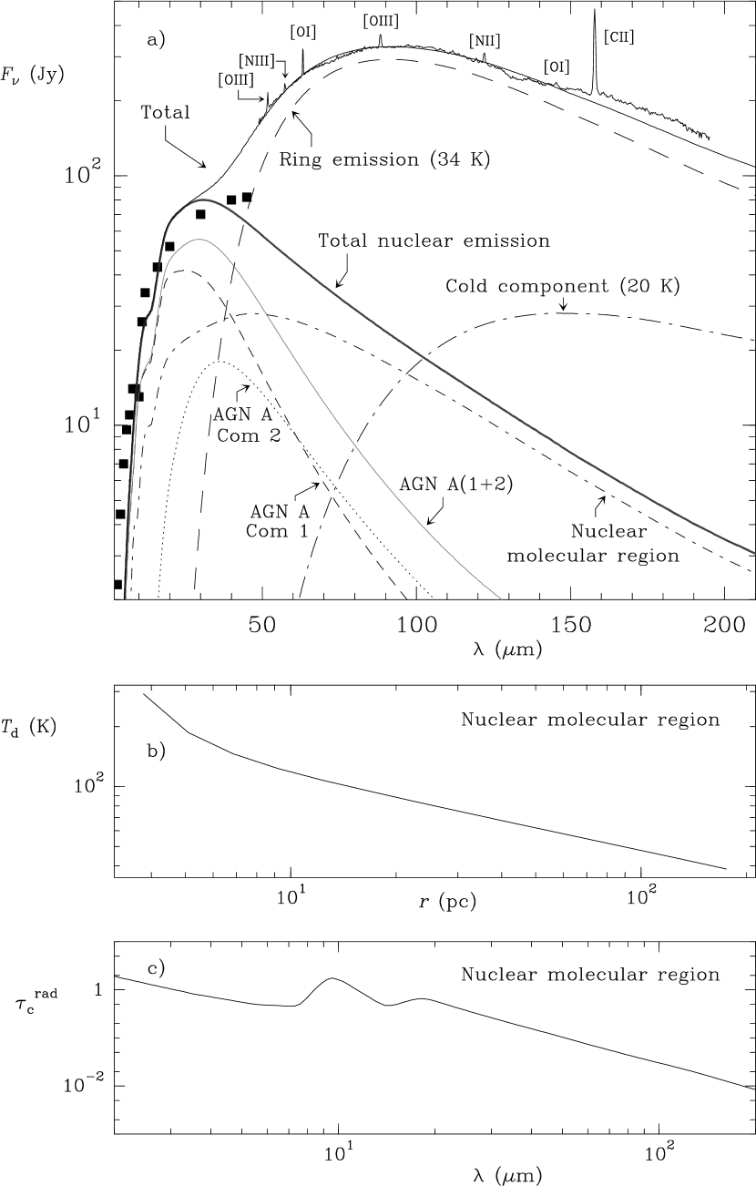
Figure 4.— a) Spectral energy distribution of NGC 1068 and model fit. ISO-SWS fluxes are taken from Lutz et al. (2000). The model fit is the composition of $(i)$ the NLR components 1 & 2 of model AGN A, $(ii)$ the emission from the molecular nuclear region, $(iii)$ the 34 K starburst emission, and $(iv)$ the cold 20 K component. b) and c) Dust temperature versus the radial position and radial continuum opacity versus wavelength for the nuclear molecular region.

Figure 5.— Energy level diagram of OH. Rotational levels with energies up to 600 K are shown; the three lines detected in NGC 1068 are indicated with arrows, as well as the 35 and 53 $\mu$m lines that could play an important role in the radiative excitation. The wavelengths are indicated in $\mu$m. $\Lambda$-doubling is ignored because the $\Lambda$-doublets are not resolved with the ISO grating resolution.

Figure 6.— Comparison between the observed OH lines and model results. As indicated in the upper panel, the upper modeled spectrum (solid lines) corresponds to the model for the nucleus, the middle one (dotted lines) corresponds to the starburst modelled as a whole, and the lower one (dashed lines) corresponds to the starburst modelled as an ensemble of individual clouds (see text for details).

Table 1Measured line fluxes from the LWS and SWS grating spectra, with 1$\sigma$ uncertainties.

Line	$\lambda$	Flux	Aperture	reference
	($\mu$m)	$(10^{-13}~{}erg~{}s^{-1}~{}cm^{-2})$	$(\arcsec^{2})$
${\rm[Si~{}IX]}$ ${}^{3}P_{2}\rightarrow{{}^{3}P_{1}}$	2.584	3.0	14 $\times$ 20	1
${\rm[Mg~{}VIII]}$ ${}^{2}P_{3/2}\rightarrow{{}^{2}P_{1/2}}$	3.028	11. $\pm$ 1.1	14 $\times$ 20	1
${\rm[Si~{}IX]}$ ${}^{3}P_{1}\rightarrow{{}^{3}P_{0}}$	3.936	5.0 $\pm$ 0.6	14 $\times$ 20	1
${\rm[Mg~{}IV]}$ ${}^{2}P_{1/2}\rightarrow{{}^{2}P_{3/2}}$	4.487	7.6 $\pm$ 1.5	14 $\times$ 20	1
${\rm[Ar~{}VI]}$ ${}^{2}P_{3/2}\rightarrow{{}^{2}P_{1/2}}$	4.529	15. $\pm$ 3.	14 $\times$ 20	1
${\rm[Fe~{}II]}$ ${}^{a4}F_{9/2}\rightarrow{{}^{a6}D_{9/2}}$	5.340	5.0	14 $\times$ 20	1
${\rm[Mg~{}VII]}$ ${}^{3}P_{2}\rightarrow{{}^{3}P_{1}}$	5.503	13.	14 $\times$ 20	1
${\rm[Mg~{}V]}$ ${}^{3}P_{1}\rightarrow{{}^{3}P_{2}}$	5.610	18. $\pm$ 2.	14 $\times$ 20	1
${\rm[Ar~{}II]}$ ${}^{2}P_{1/2}\rightarrow{{}^{2}P_{3/2}}$	6.985	13.	14 $\times$ 20	1
${\rm[Na~{}III]}$ ${}^{2}P_{1/2}\rightarrow{{}^{2}P_{3/2}}$	7.318	5.8	14 $\times$ 20	1
${\rm[Ne~{}VI]}$ ${}^{2}P_{3/2}\rightarrow{{}^{2}P_{1/2}}$	7.652	110. $\pm$ 11.	14 $\times$ 20	1
${\rm[Fe~{}VII]}$ ${}^{3}F_{4}\rightarrow{{}^{3}F_{3}}$	7.815	3.0	14 $\times$ 20	1
${\rm[Ar~{}V]}$ ${}^{3}P_{2}\rightarrow{{}^{3}P_{1}}$	7.902	$<$ 12.	14 $\times$ 20	1
${\rm[Na~{}VI]}$ ${}^{3}P_{2}\rightarrow{{}^{3}P_{1}}$	8.611	$<$ 16.	14 $\times$ 20	1
${\rm[Ar~{}III]}$ ${}^{3}P_{1}\rightarrow{{}^{3}P_{2}}$	8.991	23.0 $\pm$ 3.3	14 $\times$ 20	1
${\rm[Fe~{}VII]}$ ${}^{3}F_{3}\rightarrow{{}^{3}F_{2}}$	9.527	4.0	14 $\times$ 20	1
${\rm[S~{}IV]}$ ${}^{2}P_{3/2}\rightarrow{{}^{2}P_{1/2}}$	10.510	58. $\pm$ 6.	14 $\times$ 20	1
${\rm[Ne~{}II]}$ ${}^{2}P_{3/2}\rightarrow{{}^{2}P_{1/2}}$	12.813	70.	14 $\times$ 27	1
${\rm[Ar~{}V]}$ ${}^{3}P_{1}\rightarrow{{}^{3}P_{0}}$	13.102	$<$ 16.	14 $\times$ 27	1
${\rm[Ne~{}V]}$ ${}^{3}P_{2}\rightarrow{{}^{3}P_{1}}$	14.322	97. $\pm$ 9.7	14 $\times$ 27	1
${\rm[Ne~{}III]}$ ${}^{3}P_{1}\rightarrow{{}^{3}P_{2}}$	15.555	160. $\pm$ 32.	14 $\times$ 27	1
${\rm[Fe~{}II]}$ ${}^{a4}F_{7/2}\rightarrow{{}^{a4}F_{9/2}}$	17.936	$<$ 10.	14 $\times$ 27	1
${\rm[S~{}III]}$ ${}^{3}P_{2}\rightarrow{{}^{3}P_{1}}$	18.713	40.	14 $\times$ 27	1
${\rm[Ne~{}V]}$ ${}^{3}P_{1}\rightarrow{{}^{3}P_{0}}$	24.317	70. $\pm$ 7.	14 $\times$ 27	1
${\rm[O~{}IV]}$ ${}^{2}P_{3/2}\rightarrow{{}^{2}P_{1/2}}$	25.890	190. $\pm$ 20.	14 $\times$ 27	1
${\rm[Fe~{}II]}$ ${}^{a6}D_{7/2}\rightarrow{{}^{a6}D_{9/2}}$	25.988	8.	14 $\times$ 27	1
${\rm[S~{}III]}$ ${}^{3}P_{1}\rightarrow{{}^{3}P_{0}}$	33.481	55.	20 $\times$ 33	1
${\rm[Si~{}II]}$ ${}^{2}P_{3/2}\rightarrow{{}^{2}P_{1/2}}$	34.814	91.	20 $\times$ 33	1
${\rm[Ne~{}III]}$ ${}^{3}P_{0}\rightarrow{{}^{3}P_{1}}$	36.013	18.	20 $\times$ 33	1
${\rm[O~{}III]}$ ${}^{3}P_{2}\rightarrow{{}^{3}P_{1}}$	51.814	114. $\pm$ 3.	80	2
${\rm[N~{}III]}$ ${}^{2}P_{3/2}\rightarrow{{}^{2}P_{1/2}}$	57.317	51.4 $\pm$ 2.5	80	2
${\rm[O~{}I]}$ ${}^{3}P_{1}\rightarrow{{}^{3}P_{2}}$	63.184	156. $\pm$ 1.	80	2
${\rm[O~{}III]}$ ${}^{3}P_{1}\rightarrow{{}^{3}P_{0}}$	88.356	111. $\pm$ 1.	80	2
${\rm[N~{}II]}$ ${}^{3}P_{2}\rightarrow{{}^{3}P_{1}}$	121.897	30.5 $\pm$ 1.1	80	2
${\rm[O~{}I]}$ ${}^{3}P_{0}\rightarrow{{}^{3}P_{1}}$	145.525	11.9 $\pm$ 0.4	80	2
${\rm[C~{}II]}$ ${}^{2}P_{3/2}\rightarrow{{}^{2}P_{1/2}}$	157.741	216. $\pm$ 1.	80	2
OH ${}^{2}\Pi_{1/2}$5/2-${}^{2}\Pi_{3/2}$3/2	34.60/34.63	$<$ 3.	20 $\times$ 33	2
OH ${}^{2}\Pi_{1/2}$1/2-${}^{2}\Pi_{1/2}$3/2	79.11/79.18	14.4 $\pm$ 1.5	80	2
OH ${}^{2}\Pi_{3/2}$5/2-${}^{2}\Pi_{3/2}$3/2	119.23/119.44	11.9 $\pm$ 1.2	80	2
OH ${}^{2}\Pi_{1/2}$3/2-${}^{2}\Pi_{1/2}$1/2	163.12/163.40	7.42 $\pm$ 0.65	80	2

Note. — (1): from Lutz et al. (2000) and, where errors are available, Alexander et al. (2000); (2): this work

Table 2Comparison of observed line fluxes with AGN model predictions

Line id.$\lambda$	Flux (${\rm 10^{-13}~{}erg~{}s^{-1}~{}cm^{-2}}$)
($\mu$m )	Observed/D /D	AGN A model		AGN B model		AGN C model
		Comp. 1	Comp. 2	Comp. 1	Comp. 2	Comp. 1	Comp. 2
${\rm O~{}VI}$ ${\lambda}$ .1032+.1037	37.4/4334./402.	32.6+19.8	2.28+1.94	8.26+5.36	0.31+0.27	56.7+31.2	3.41+2.10
${\rm(Ly\alpha)_{n}}$ $\lambda$ .1215	101.8/3562./602	179	619	149.	500	239.	638.
${\rm N~{}IV]}$ $\lambda$ .1487	5.1/103./22.9	25.2	6.64	36.3	6.28	59.6	47.5
${\rm(CIV)_{n}}$ $\lambda$ .1549	39.7/790./177.	142.	77.6	110.9	56.5	286.	329.
${\rm HeII}$ $\lambda$ .1640	21.4/426./95.5	112.	85.9	108	81.8	346.	345.
${\rm[Ne~{}V]}$ $\lambda$ .3426	15.7/95./38.7	97.7	23.3	68.2	7.36	271.	115
${\rm[Ne~{}III]}$ $\lambda$ .3869+.3968	19.2/97./43.2	37.1+11.2	41.5+12.5	102.8+31.0	102.+30.7	81.6+24.6	143.+43.0
${\rm HeII}$ $\lambda$ .4686	6.1/27.6/13.	15.0	12.3	14.7	11.8	46.5	48.4
${\rm[O~{}III]}$ $\lambda$ .4959+.5007	256./964./496	86.9+262	99.5+294	197.+593	185.+557.	148.+446.	241+726
${\rm[Si~{}VI]}$ $\lambda$ 1.96	8.0/9.2/8.6	11.2	1.53	10.8	1.86	23.3	3.74
${\rm[Si~{}VII]}$ $\lambda$ 2.48	8.3	6.41	0.1	9.12	0.18	11.0	0.22
${\rm[Si~{}IX]}$ $\lambda$ 2.584	3.0	0.49	—	0.84	—	0.32	—
${\rm[Mg~{}VIII]}$ $\lambda$ 3.028	11.	2.97	—	4.80	—	4.29	—
${\rm[Si~{}IX]}$ $\lambda$ 3.936	5.4	0.89	—	1.56	—	0.56	—
${\rm[Mg~{}IV]}$ $\lambda$ 4.487	7.6	3.85	7.98	4.29	6.92	9.80	19.5
${\rm[Ar~{}VI]}$ $\lambda$ 4.529	15.	10.3	4.0	13.4	3.10	26.2	20.1
${\rm[Mg~{}VII]}$ $\lambda$ 5.503	13.	9.68	0.13	11.4	.075	20.0	0.45
${\rm[Mg~{}V]}$ $\lambda$ 5.610	18.	10.7	8.63	7.85	3.84	34.6	29.5
${\rm[Ar~{}II]}$ $\lambda$ 6.985	13.	4.56	7.53	0.93	1.36	0.87	1.63
${\rm[Na~{}III]}$ $\lambda$ 7.318	5.8	0.56	0.59	1.27	1.51	0.67	1.21
${\rm[Ne~{}VI]}$ $\lambda$ 7.652	110.	153.7	11.9	105.4	3.2	393.	62.4
${\rm[Fe~{}VII]}$ $\lambda$ 7.815	3.0	1.83	1.63	1.65	0.71	6.34	6.30
${\rm[Ar~{}V]}$ $\lambda$ 7.902	$<$ 12.	2.14	1.83	2.62	1.92	3.72	6.52
${\rm[Na~{}VI]}$ $\lambda$ 8.611	$<$ 16.	1.20	0.16	0.95	—	2.95	0.65
${\rm[Ar~{}III]+[Mg~{}VII]}$ $\lambda$ 8.991	25.	4.63+11.7	7.34+0.17	5.97+14.1	12.4+0.10	4.83+23.8	10.7+0.58
${\rm[Fe~{}VII]}$ $\lambda$ 9.527	4.0	7.50	7.0	6.75	3.08	25.8	26.6
${\rm[S~{}IV]}$ $\lambda$ 10.510	58.	38.4	60.5	85.3	126.	75.8	187.
${\rm[Ne~{}II]}$ $\lambda$ 12.813	70.	5.86	20.8	2.20	4.44	1.62	3.26
${\rm[Ar~{}V]}$ $\lambda$ 13.102	$<$ 16.	2.23	2.73	2.75	2.88	3.93	9.57
${\rm[Ne~{}V]}$ $\lambda$ 14.322	97.	91.4	66.8	83.2	28.7	270.	273.
${\rm[Ne~{}III]}$ $\lambda$ 15.555	160.	44.4	52.0	76.	110.	42.0	86.9
${\rm[S~{}III]}$ $\lambda$ 18.713	40.	25.8	56.0	21.7	75.7	18.4	64.5
${\rm[Ne~{}V]}$ $\lambda$ 24.317	70.	40.8	52.6	35.8	22.1	116.	215.
${\rm[O~{}IV]}$ $\lambda$ 25.890	190.	24.1	71.9	28.3	69.7	56.4	240.
${\rm[S~{}III]}$ $\lambda$ 33.481	55.	8.00	29.8	5.57	41.1	4.84	38.4
${\rm[Si~{}II]}$ $\lambda$ 34.814	91.	12.9	22.6	6.01	24.2	5.28	29.4
${\rm[Ne~{}III]}$ $\lambda$ 36.013	18.	3.32	4.4	5.74	9.40	3.20	7.46
${\rm[O~{}III]}$ $\lambda$ 51.814	110.	9.04	33.9	16.3	63.2	9.06	48.5
${\rm[N~{}III]}$ $\lambda$ 57.317	51.	2.23	11.4	2.83	18.9	1.88	16.1
${\rm[O~{}I]}$ $\lambda$ 63.184	156.	3.84	1.8	1.57	2.26	1.24	3.10
${\rm[O~{}III]}$ $\lambda$ 88.356	110.	1.22	8.2	2.25	15.5	1.23	12.6
${\rm[N~{}II]}$ $\lambda$ 121.897	30.	0.28	0.87	.07	0.40	.06	0.52
${\rm[O~{}I]}$ $\lambda$ 145.525	12.	0.24	0.14	.09	0.18	.07	0.24
${\rm[C~{}II]}$ $\lambda$ 157.741	220.	0.50	1.58	0.18	0.97	.14	1.09

Table 3Comparison of observed line fluxes with the Ring Starburst model predictions

Line id.$\lambda$	Flux (${\rm 10^{-13}~{}erg~{}s^{-1}~{}cm^{-2}}$)
($\mu$m )	Observed	SBR A	SBR B	SBR C	SBR D	SBR E	SBR F
${\rm O~{}VI}$ ${\lambda}$ .1032+.1037	37.4/4334./402.	—	—	—	—	—	—
${\rm(Ly\alpha)_{n}}$ $\lambda$ .1215	101.8/3562./602	1330.	865.	997.	875.	1010.	917.
${\rm N~{}IV]}$ $\lambda$ .1487	5.1/103./22.9	71.9	0.20	85.8	.020	93.7	0.03
${\rm(CIV)_{n}}$ $\lambda$ .1549	39.7/790./177.	795.	0.70	858.	0.80	924.	0.87
${\rm HeII}$ $\lambda$ .1640	21.4/426./95.5	693.	50.2	696.	50.5	696.	50.8
${\rm[Ne~{}V]}$ $\lambda$ .3426	15.7/95./38.7	58.1	—	69.6	—	73.9	—
${\rm[Ne~{}III]}$ $\lambda$ .3869+.3968	19.2/97./43.2	314.+94.7	31.1+9.4	309.+93.1	31.5+9.5	316.+95.7	32.+9.7
${\rm HeII}$ $\lambda$ .4686	6.1/27.6/13.	97.3	7.4	97.7	7.4	97.3	7.4
${\rm[O~{}III]}$ $\lambda$ .4959+.5007	256./964./496	1330.+3990.	25.1+75.6	1383+4158.	26.0+78.2	1412.+4257.	26.8+80.5
${\rm[Si~{}VI]}$ $\lambda$ 1.96	8.0/9.2/8.6	—	—	—	—	—	—
${\rm[Si~{}VII]}$ $\lambda$ 2.48	8.3	—	—	—	—	—	—
${\rm[Si~{}IX]}$ $\lambda$ 2.584	3.0	—	—	—	—	—	—
${\rm[Mg~{}VIII]}$ $\lambda$ 3.028	11.	—	—	—	—	—	—
${\rm[Si~{}IX]}$ $\lambda$ 3.936	5.4	—	—	—	—	—	—
${\rm[Mg~{}IV]}$ $\lambda$ 4.487	7.6	3.30	—	3.50	—	3.53	—
${\rm[Ar~{}VI]}$ $\lambda$ 4.529	15.	6.20	—	7.72	—	8.02	—
${\rm[Mg~{}VII]}$ $\lambda$ 5.503	13.	—	—	—	—	—	—
${\rm[Mg~{}V]}$ $\lambda$ 5.610	18.	3.10	—	3.63	—	3.73	—
${\rm[Ar~{}II]}$ $\lambda$ 6.985	13.	5.90	3.70	4.29	3.70	4.12	3.73
${\rm[Na~{}III]}$ $\lambda$ 7.318	5.8	0.60	0.10	0.54	0.11	0.54	0.11
${\rm[Ne~{}VI]}$ $\lambda$ 7.652	110.	16.9	—	21.1	—	21.8	—
${\rm[Fe~{}VII]}$ $\lambda$ 7.815	3.0	0.40	—	0.48	—	0.50	—
${\rm[Ar~{}V]}$ $\lambda$ 7.902	$<$12.	7.50	—	8.84	—	9.11	—
${\rm[Na~{}VI]}$ $\lambda$ 8.611	$<$16.	—	—	—	—	—	—
${\rm[Ar~{}III]+[Mg~{}VII]}$ $\lambda$ 8.991	25.	46.5	7.10	43.2	7.13	42.2	7.13
${\rm[Fe~{}VII]}$ $\lambda$ 9.527	4.0	1.70	—	2.04	—	2.11	—
${\rm[S~{}IV]}$ $\lambda$ 10.510	58.	312.	0.80	346.	0.84	333.	0.81
${\rm[Ne~{}II]}$ $\lambda$ 12.813	70.	7.80	5.50	5.44	5.38	5.38	5.61
${\rm[Ar~{}V]}$ $\lambda$ 13.102	$<$16.	21.9	—	25.5	—	24.9	—
${\rm[Ne~{}V]}$ $\lambda$ 14.322	97.	271.	—	315.	—	314.	—
${\rm[Ne~{}III]}$ $\lambda$ 15.555	160.	295.	50.5	276.	50.2	270.	49.8
${\rm[S~{}III]}$ $\lambda$ 18.713	40.	180.	19.2	178.	20.3	203.	23.7
${\rm[Ne~{}V]}$ $\lambda$ 24.317	70.	303.	—	346.	—	294.	—
${\rm[OIV]}$ $\lambda$ 25.890	190.	1660.	1.90	1762.	2.00	1419.	1.62
${\rm[S~{}III]}$ $\lambda$ 33.481	55.	785.	87.5	673.	81.2	350.	46.2
${\rm[Si~{}II]}$ $\lambda$ 34.814	91.	126.	54.8	89.4	49.5	41.9	29.4
${\rm[Ne~{}III]}$ $\lambda$ 36.013	18.	52.8	8.90	49.2	8.91	47.5	8.74
${\rm[O~{}III]}$ $\lambda$ 51.814	110.	2980.	81.5	3217	87.5	2524.	71.9
${\rm[N~{}III]}$ $\lambda$ 57.317	51.	1110.	40.0	921	35.0	372.9	14.7
${\rm[O~{}I]}$ $\lambda$ 63.184	156.	165.	130.	113.	127.	116.	124.
${\rm[O~{}III]}$ $\lambda$ 88.356	110.	4980.	138.	3729.	109.	977.	29.0
${\rm[N~{}II]}$ $\lambda$ 121.897	30.	80.0	37.3	47.8	29.7	12.3	8.78
${\rm[O~{}I]}$ $\lambda$ 145.525	12.	16.2	12.9	11.0	12.5	10.1	11.3
${\rm[C~{}II]}$ $\lambda$ 157.741	220.	739.	465.	181.	172.	67.6	46.5

Note. — *: this line was used for normalization

Table 4Comparison of observed line fluxes with composite model predictions

Line id.$\lambda$	Flux (${\rm 10^{-13}~{}erg~{}s^{-1}~{}cm^{-2}}$)
($\mu$m )	Observed/D /D	CM1	CM2	CM3
${\rm O~{}VI}$ $\lambda$ .1032+.1037	37.4/4334./402.	56.6	14.2	93.4
${\rm(Ly\alpha)_{n}}$ $\lambda$ .1215	101.8/3562./602	1673.	1524.	1752.
${\rm N~{}IV]}$ $\lambda$ .1487	5.1/103./22.9	31.8	42.6	107.
${\rm(CIV)_{n}}$ $\lambda$ .1549	39.7/790./177.	220.	168.	616.
${\rm HeII}$ $\lambda$ .1640	21.4/426./95.5	248.	240.	741.
${\rm[Ne~{}V]}$ $\lambda$ .3426	15.7/95./38.7	121.	75.6	386.
${\rm[Ne~{}III]}$ $\lambda$ .3869+.3968	19.2/97./43.2	143.	307.	333.
${\rm HeII}$ $\lambda$ .4686	6.1/27.6/13.	34.7	33.9	102.3
${\rm[O~{}III]}$ $\lambda$ .4959+.5007	256./964./496	847.	1636.	1665.
${\rm[Si~{}VI]}$ $\lambda$ 1.96	8.0/9.2/8.6	12.7	12.7	27.0
${\rm[Si~{}VII]}$ $\lambda$ 2.48	8.3	6.5	9.3	11.2
${\rm[Si~{}IX]}$ $\lambda$ 2.584	3.0	0.5	0.8	0.3
${\rm[Mg~{}VIII]}$ $\lambda$ 3.028	11.	3.0	4.8	4.3
${\rm[Si~{}IX]}$ $\lambda$ 3.936	5.4	0.9	1.6	0.6
${\rm[Mg~{}IV]}$ $\lambda$ 4.487	7.6	11.8	11.2	29.3
${\rm[Ar~{}VI]}$ $\lambda$ 4.529	15.	14.3	16.5	46.3
${\rm[Mg~{}VII]}$ $\lambda$ 5.503	13.	9.8	11.5	20.5
${\rm[Mg~{}V]}$ $\lambda$ 5.610	18.	19.3	11.7	64.1
${\rm[Ar~{}II]}$ $\lambda$ 6.985	13.	15.8	6.0	6.2
${\rm[Na~{}III]}$ $\lambda$ 7.318	5.8	1.3	2.8	2.0
${\rm[Ne~{}VI]}$ $\lambda$ 7.652	110.	166.	109.	455.
${\rm[Fe~{}VII]}$ $\lambda$ 7.815	3.0	3.5	2.4	12.6
${\rm[Ar~{}V]}$ $\lambda$ 7.902	$<$12.	4.0	4.5	10.2
${\rm[Na~{}VI]}$ $\lambda$ 8.611	$<$16.	1.4	0.9	3.6
${\rm[Ar~{}III]+[Mg~{}VII]}$ $\lambda$ 8.991	25.	31.	39.7	47.0
${\rm[Fe~{}VII]}$ $\lambda$ 9.527	4.0	14.5	9.8	52.4
${\rm[S~{}IV]}$ $\lambda$ 10.510	58.	99.7	212.	263.
${\rm[Ne~{}II]}$ $\lambda$ 12.813	70.	32.0	12.0	10.3
${\rm[Ar~{}V]}$ $\lambda$ 13.102	$<$16.	5.0	5.6	13.5
${\rm[Ne~{}V]}$ $\lambda$ 14.322	97.	158.	112.	543.
${\rm[Ne~{}III]}$ $\lambda$ 15.555	160.	147.	236.	179.
${\rm[S~{}III]}$ $\lambda$ 18.713	40.	102.	118.	103.
${\rm[Ne~{}V]}$ $\lambda$ 24.317	70.	93.4	57.9	331.
${\rm[O~{}IV]}$ $\lambda$ 25.890	190.	98.	100.	298.
${\rm[S~{}III]}$ $\lambda$ 33.481	55.	119.	128.	124.
${\rm[Si~{}II]}$ $\lambda$ 34.814	91.	85.	79.7	84.2
${\rm[Ne~{}III]}$ $\lambda$ 36.013	18.	16.6	24.0	19.6
${\rm[O~{}III]}$ $\lambda$ 51.814	110.	130.	167.	145.
${\rm[N~{}III]}$ $\lambda$ 57.317	51.	48.6	56.7	53.
${\rm[O~{}I]}$ $\lambda$ 63.184	156.	133.	131.	131.
${\rm[O~{}III]}$ $\lambda$ 88.356	110.	118.	127.	123.
${\rm[N~{}II]}$ $\lambda$ 121.897	30.	30.8	30.	30.3
${\rm[O~{}I]}$ $\lambda$ 145.525	12.	12.9	12.8	12.8
${\rm[C~{}II]}$ $\lambda$ 157.741	220.	174.	173.	173.

Table 5Comparison of observed line fluxes with model predictions for the nuclear region

Line id.$\lambda$	Flux ($10^{-12}~{}erg~{}s^{-1}~{}cm^{-2}$)		Notes
	Observed	Modeled
34$\mu$m	$<$ 0.1	-0.43	(absorption)
53$\mu$m	$<$ 1.2	-0.66	(absorption)
79$\mu$m	1.1	1.13
84$\mu$m	$<$ 1.2	0.06
98$\mu$m	$<$ 1.2	0.17
119$\mu$m	1.3	1.60
163$\mu$m	0.38	0.35

References

- Alexander et al. (2000) Alexander, T., Lutz, D., Sturm, E., Genzel, R., Sternberg, A., Netzer, H. 2000, ApJ, 536, 710.
- Alloin et al. (2001) Alloin, D., Galliano, E., Cuby, J. G., Marco, O., Rouan, D., Cl net, Y., Granato, G. L., Franceschini, A. 2001, A&A, 369, L33.
- Ashby et al. (2000) Ashby, M., et al. 2000, ApJ, 539, L119
- Bernes (1979) Bernes, C. 1979, A&A, 73, 67.
- Bland-Hawthorn et al. (1997) Bland-Hawthorn, J., Gallimore, J. F., Tacconi, L. J., Brinks, E., Baum, S. A., Antonucci, R. R. J., Cecil, G. N. 1997, Ap&SS, 248, 9.
- Blietz et al. (1994) Blietz, M., Cameron, M., Drapatz, S., Genzel, R., Krabbe, A., van der Werf, P., Sternberg, A., Ward, M. 1994, ApJ, 421, 92.
- Bradford et al. (1999) Bradford, C.M., et al., 1999, Proc.of the Conference “The Universe as seen by ISO”, Paris, France, 20-23 October 1998 (ESA SP-427),p.861.
- Cameron et al. (1993) Cameron, M., Storey, J.W.V., Rotaciuc, V., Genzel, R., Verstraete, L., Drapatz, S., Siebenmorgen, R., Lee, T. J. 1993, ApJ, 419, 136
- Clegg et al. (1996) Clegg, P.E., et al. 1996, A&A, 315, L28.
- Colbert et al. (1999) Colbert, J., et al., 1999, ApJ, 511, 721.
- Davies, Sugai & Ward (1998) Davies, R.I., Sugai,H., and Ward, M.J., 1998, MNRAS, 300, 388
- Draine (1985) Draine, B. T. 1985, ApJSS, 57, 587.
- Ferland et al. (1998) Ferland, G. J., Korista, K. T., Verner, D. A., Ferguson, J. W., Kingdon, J. B., Verner, E. M. 1998, PASP, 110, 761.
- Ferland (2000) Ferland, G.J., 2000, RevMexAA,(Serie de Conferencias), Vol.9, 153
- Fischer et al. (1999) Fischer, J., et al. 1999, Ap&SS, 266, 91.
- Goicoechea & Cernicharo (2002) Goicoechea, J. R., Cernicharo, J. 2002, ApJ, 576, 77.
- González-Alfonso & Cernicharo (1997) González-Alfonso, E., & Cernicharo, J. 1997, A&A, 322, 938
- González-Alfonso & Cernicharo (1999) González-Alfonso, E., & Cernicharo, J. 1999, ApJ, 525, 845
- González-Alfonso et al. (2004) González-Alfonso, E., Smith, H.A., Fischer, J., Cernicharo, J. 2004, ApJ, 613, 247.
- Harvey et al. (1999) Harvey, V.I., et al., 1999, Proc.of the Conference ”The Universe as seeen by ISO”, Paris, France, 20-23 October 1998 (ESA SP-427), p.889.
- Helfer & Blitz (1995) Helfer, T.T., Blitz, L., 1995, ApJ, 450, 90.
- Huchra et al. (1999) Huchra, J.P., Vogeley, M.S. & Geller, M.J. 1999, ApJS, 121, 287.
- Kaufman et al. (1999) Kaufman, M.J., Wolfire, M.G., Hollenbach, D.J., Luhman, M.L. 1999, ApJ, 527, 795.
- Kessler et al. (1996) Kessler, M.F. et al.,1996, A&A, 315, L27
- Kriss et al. (1992) Kriss, G. A., Davidsen, A. F., Blair, W. P., Ferguson, H. C., Long, K. S. 1992, ApJ, 394, L37
- Krolik & Lepp (1989) Krolik, J.H., & Lepp, S. 1989, ApJ, 347, 179
- Ivezic & Elitzur (1997) Ivezic, Z., & Elitzur, M. 1997, MNRAS, 287, 799
- Le Floc’h et al. (2001) Le Floc’h, E., Mirabel, I.F., Laurent, O., Charmandaris, V. et al. 2001, A&A, 367, 487.
- Leitherer et al. (1999) Leitherer, C., et al. 1999, ApJS, 125, 489.
- Lepp & Dalgarno (1996) Lepp, S., Dalgarno, A. 1996, A&A, 306, 21.
- Luhman et al. (2003) Luhman, M. L., Satyapal, S., Fischer, J., Wolfire, M. G., Sturm, E., Dudley, C. C., Lutz, D., Genzel, R. 2003, ApJ, 594, 758.
- Lutz et al. (2000) Lutz, D. et al., 2000,ApJ, 536, 697.
- Malhotra et al. (2001) Malhotra, S. et al. 2001, ApJ, 561, 766.
- Maloney et al. (1996) Maloney, P.R., Hollenbach, D.J., Tielens, A.G.G.M. 1996, ApJ, 466, 561.
- Marconi et al. (1996) Marconi, A., van der Werf, P. P., Moorwood, A. F. M., Oliva, E. 1996, A&A, 315, 335.
- Malkan & Oke (1983) Malkan, M. A. & Oke, J. B. 1983, ApJ, 265, 92.
- Offer et al. (1994) Offer, A.R., van Hemert, M.C., & van Dishoeck, E.F. 1994, J. Chem. Phys., 100, 362.
- Papadopoulos & Seaquist (1999a) Papadopoulos,P.P. & Seaquist, E.R. 1999, ApJ, 514,L95.
- Papadopoulos & Seaquist (1999b) Papadopoulos,P.P. & Seaquist, E.R. 1999, ApJ, 516,114.
- Pier et al. (1994) Pier, E.A., Antonucci, R. H., Hurt, T.; Kriss, G.; Krolik, J. 1994, ApJ, 428, 124.
- Planesas et al. (1991) Planesas, P., Scoville, N., & Myers, S.T. 1991, ApJ, 369, 364.
- Preibisch et al. (1993) Preibisch, T., Ossenkopf, V., Yorke, H.W., Henning, T. 1993, A&A, 279, 577.
- Rotaciuc et al. (1991) Rotaciuc, V., Krabbe, A., Cameron, M., Drapatz, S. et al. 1991, ApJ, 370, 23.
- Schinnerer et al. (2000) Schinnerer, E., Eckart, A., Tacconi, L.J., Genzel, R., & Downes, D. 2000, ApJ, 533, 850.
- Smith (2004) Smith, H.A. 2004, in “Second Workshop on New Concepts for Far Infrared and Submillimeter Space Astronomy”, 7-8 March 2002, Univ. Maryland, College Park, Maryland, eds. D. Benford & D. Leisawitz, NASA/CP-2003-212233, p. 98.
- Smith et al. (2004) Smith, H. A., et al., 2004, in prep.
- Spinoglio, Andreani & Malkan (2002) Spinoglio, L., Andreani, P. & Malkan, M.A., 2002, ApJ, 572, 105.
- Spinoglio & Malkan (1992) Spinoglio, L. & Malkan, M.A.,1992, ApJ,399,504.
- Scoville et al. (1988) Scoville, N.Z., Matthews, K., Carico, D.P., Sanders, D.B. 1988, ApJ, 327, L61.
- Sternberg & Dalgarno (1995) Sternberg, A., Dalgarno, A. 1995, ApJSS, 99, 565.
- Sternberg et al. (1994) Sternberg, A., Genzel, R., Tacconi, L. 1994, ApJ, 436, 131.
- Swinyard et al. (1996) Swinyard, B.M., et al. 1996, A&A, 315, L43.
- Swinyard et al. (1998) Swinyard, B.M., et al. 1998, Proc. SPIE, A.M. Fowler (Ed.), Vol.3354, P.888.
- Tacconi et al. (1994) Tacconi, L. J., Genzel, R., Blietz, M., Cameron, M., Harris, A. I., Madden, S. 1994, ApJ, 426, 77.
- Telesco et al. (1984) Telesco, C.M., Becklin, E. E., Wynn-Williams, C. G., Harper, D. A. 1984, ApJ, 282, 427.
- Thatte et al. (1997) Thatte, N., Quirrenbach, A., Genzel, R., Maiolino, R., Tecza, M. 1997, ApJ, 490, 238.
- Thompson (1996) Thompson, R.I., 1996, ApJ, 459, L61.
- Thronson et al. (1989) Thronson,H.A. et al. 1989, ApJ, 343, 158.
- Usero et al. (2004) Usero, A., García-Burillo, S., Fuente, A., Martín-Pintado, J., Rodríguez-Fernández, N.J. 2004, A&A, 419, 897