Evidence for transient clumps and gas chemical evolution in the CS core of L673

We present FCRAO maps as well as combined BIMA and FCRAO maps of the high density molecular emission towards the CS core in the L673 region. With the FCRAO telescope we mapped the emission in the CS (2$\rightarrow 1$), C³⁴S (2$\rightarrow 1$), HCO⁺ (1$\rightarrow 0$), and H¹³CO⁺ (1$\rightarrow 0$) lines. The high-density molecular emission, which arises from a filamentary structure oriented in the NW-SE direction, shows clear morphological differences for each molecule. We find that HCO⁺ has an extremely high optical depth, and that the H¹³CO⁺ emission is well correlated with submm sources. The BIMA and FCRAO combined maps recover emission from structure previously undetected or marginally detected, and show an overall aspect of a filamentary structure connecting several intense clumps. We found a total 15 clumps in our combined data cube, all of them resolved at our angular resolution, with diameters in the 0.03–0.09 pc range. Their estimated masses range between 0.02 and 0.2 $M_{\sun}$, except for the largest clump, which has a mass of $\sim 1.2$ $M_{\sun}$. We find a clear segregation between the northern and southern region of the map: the northern section shows the less chemically evolved gas and less massive but more numerous clumps, while the southern region is dominated by the largest and most massive clump, and contains the more evolved gas, as traced by emission of late-time molecules. We find that the derived clump masses are below the virial mass, and that the clump masses become closer to the virial mass when they get bigger and more massive. This supports the idea that these clumps must be transient, and that only the more massive ones are able to condense into stars. The clumps we detect are probably in an earlier evolutionary stage than the “starless cores” reported recently in the literature. Only the most massive one has properties similar to a “starless core”.

1 Introduction

Dense cores of molecular clouds have been extensively used to study the star formation process. The emission of several molecules known to be good tracers of high density molecular gas has been used to study their properties, such as mass and density, temperature, and velocity distributions. However, it was apparent from the first surveys (Zhou et al. zhou (1989); Myers et al. myers (1991)) that there existed large discrepancies between the emission of some of these molecules, such as CS, NH₃ or HCO⁺, which needed to be clarified in order to obtain the actual distribution of the high density gas in these sources. Pastor et al. (Pastor91 (1991)) and Morata et al. (Morata97 (1997)) carried out a systematic comparison between the emission of the CS ($J$=1$\rightarrow$0) and NH₃ ($J,K$)=(1,1) transitions, under similar conditions of angular resolution, which confirmed these discrepancies, in particular the systematic difference in size and separation between the emission peaks of both molecules.

To explain these results, Taylor et al. (Taylor96 (1996), Taylor98 (1998)) developed a chemical model in which high density condensations, or dense cores, are formed by clumps of different masses, ages, sizes, and densities but with sizes of $\la 0.1$ pc. These clumps would be unresolved in single-dish angular resolution observations such as the ones listed in the previous paragraph. Most of the clumps would disperse before NH₃ abundances build up to significant levels, though these clumps would contain substantial CS, so its emission should be observable. A few clumps, those sufficiently long-lived, or in a more advanced stage of physical and chemical evolution because of being denser or more massive, would form a significant amount of NH₃, while the CS abundance decreases with time. These clumps would possibly continue their evolution to eventually form stars. Moreover, Taylor et al. (Taylor96 (1996), Taylor98 (1998)) found that a classification could be made in the model between “early-time” molecules (showing extended emission like CS) and “late-time” molecules (showing more compact emission like NH₃), according to the time at which these molecules reached their peak fractional abundance.

In order to test the Taylor et al. chemical model, and in particular to study the small–size structure of the dense cores, we carried out high angular resolution observations with the BIMA telescope towards the L673 molecular cloud of several transitions corresponding to molecules of both families of species (Morata, Girart & Estalella Morata03 (2003); hereafter MGE03). The region selected had been previously mapped at an angular resolution of $\sim 1^{\prime}$ in CS (2$\rightarrow 1$) (Morata et al. Morata97 (1997)) and NH₃ ($J,K$)=(1,1) (Sepúlveda et al. in preparation). It has no signs of star formation and is located $\sim 9\aas@@fstack{\prime}5$ to the southeast of IRAS 19180$+$1116. The distance to the L673 cloud is $\sim 300$ pc (Herbig & Jones Herbig83 (1983))

MGE03 detect emission in the CS ($J$=2$\rightarrow$1), N₂H⁺ ($J$=1$\rightarrow$0), HCO⁺ ($J$=1$\rightarrow$0) and SO ($J_{K}=2_{3}\rightarrow 1_{2}$) lines. The high angular resolution interferometric observations reveal a much clumpier medium than the lower resolution single-dish observations. Several clumps of size $\la 0.08$ pc are detected distributed all over the region encompassed by the single-dish observations. However, the BIMA interferometer only detects 9–12% of the CS (2$\rightarrow$1) emission. Modelling the filtering effect of BIMA, MGE03 show that a clumpy and heterogeneous medium could explain this effect.

MGE03 find that the BIMA observations can be fitted by a model with a density at which collapse is halted of $n_{f}=5\times 10^{5}$ cm^-3. A tentative classification of the studied clumps according to the stage of chemical evolution indicated by the molecular abundances is proposed. However, the model cannot explain the observed low HCO⁺ abundances with respect to the predicted values obtained at two positions, but this is possibly due to strong self-absorption in the HCO⁺ (1$\rightarrow 0$) line.

The results of MGE03 show that although the interferometric observations lose information on the total emission of the region, they are in agreement with the results obtained with single-dish telescopes, suggesting that interferometric observations are useful for studying with high angular resolution the chemical evolution of the inner structures of starless cores. However, in order to avoid the filtering effect of interferometers, array observations should be combined with single dish observations. This would give high resolution maps of the full emission.

In this paper we present the study of the spatial distribution of the molecular emission in L673 from the maps obtained with the 14-m FCRAO telescope, and from the maps obtained by combining the BIMA data of MGE03 and the FCRAO maps presented in this paper. In Sect. 2 we describe the FCRAO observations and the BIMA and FCRAO combination procedure. In Sect. 3 we describe the morphological properties of the molecular emission. In Sect. 4 we analyze the properties of the molecular cloud observed.

2 Observations

2.1 FCRAO Observations

Table 1: Lines Observed with the 14-m FCRAO telescope

$$\!\!\!\!\nu$$ FWHM

Molecule Transition (GHz) Beam (kms) (K)

H¹³CO⁺ (1) 86.75434 59^′′ 0.17 0.04

HCO⁺ (1) 89.18852 58^′′ 0.16 0.11

C³⁴S (2) 96.41295 53^′′ 0.15 0.07

CS (2) 97.98097 52^′′ 0.15 0.14

The observations were carried out in 2003 January with the 14–m Five College Radio Astronomy Observatory (FCRAO) telescope using the SEQUOIA (Second Quabbin Observatory Imaging Array) 16 beam array receiver. We used the dual channel correlator (DCC), which provided a bandwidth of 25 MHz and a spectral resolution of 24.4 kHz. The DCC was configured to observe the 4 molecular transitions using 3 different frequency setups: one for HCO⁺, one for CS, and one for H¹³CO⁺ and C³⁴S, which were observed simultaneously. The main-beam efficiency at the frequencies observed is $\eta_{\rm mb}\simeq 0.50$. At 89 and 98 GHz the half-power beam width is $58^{\prime\prime}$ and $52^{\prime\prime}$, respectively. The weather conditions during the observations were excellent, providing averaged system temperatures of $\sim$120 K. The observations were performed using the On-The-Fly (OTF) mapping technique, covering a region of $8^{\prime}\times 8^{\prime}$ for HCO⁺ and CS and of $6^{\prime}\times 6^{\prime}$ for H¹³CO⁺ and C³⁴S. The center of the maps was $\alpha(J2000)=19^{\rm h}20^{\rm m}52\aas@@fstack{s}20$; $\delta(J2000)=11\mbox{${}^{\circ}$}14^{\prime}45\aas@@fstack{\prime\prime}5$. The selected reference position was 30^′ east of the center position. A summary of the observed molecular line transitions is given in Table 1. The OTF maps were regridded to have a cell size of 20^′′. The line intensities are given in main-beam brightness temperature, $T_{\rm mb}=T^{*}_{A}/\eta_{\rm mb}$.

2.2 Combination procedure for the FCRAO and BIMA data

The BIMA interferometer detects only 9–12% of the CS (2$\rightarrow 1$) emission. Therefore, in order to recover the missing flux of the interferometer data we combined the CS (2$\rightarrow 1$) and HCO⁺ (1$\rightarrow 0$) data obtained with the FCRAO presented in this paper with the BIMA data from MGE03. The first step to do this is to convert the FCRAO antenna temperature to a flux scale. We used a 43 Jy K^-1 conversion factor for the two transitions (M. Heyer, private communication). There are basically two single-dish and interferometric data combination techniques that work well (Helfer et al. Helfer03 (2003)). One is to add synthetic short-spacing visibilities in the $(u,v)$ plane (e. g., Vogel et al. Vogel84 (1984); Girart et al. Girart99 (1999)). The other is a linear combination procedure of the single-dish and interferometric maps (e. g., Ye, Turtle & Kennicutt Ye91 (1991); Stanimirovic et al. Stanimirovic99 (1999)). We tested these two techniques.

In order to fill the BIMA visibility hole with synthetic FCRAO visibilities, we first deconvolved the FCRAO maps from the FCRAO beam pattern using the CLEAN algorithm. The beam was modeled as a Gaussian with the FWHM given in Table 1. The deconvolved FCRAO map was then multiplied by the interferometer primary-beam response, taken as a Gaussian, and centered on the two position observed with BIMA (see MGE03). From these two resulting maps, a randomly distributed sample of visibilities was generated in the $(u,v)$ plane of 0–20 light-ns. The number of visibilities generated was chosen to have a visibility density similar to the BIMA data for the inner part of the $(u,v)$-plane. To check the relative flux calibration of the FCRAO data with the BIMA data, FCRAO visibilities were generated in the range of 21 to 30 light-ns at the same location as the BIMA visibilities. The two data sets were compared by vector-averaging the visibilities in this range over concentric annuli. The values obtained from the two instruments agreed to within 15%.

Table 2: Parameters of the FCRAO and BIMA Combined Maps

Rms

Molecular Synthesized Beam $$\!\!\!\!\Delta v$$ Noise

Transition HPBW P.A. (kms) (Jy Beam^-1)

HCO⁺ (1) 0.33 0.22

CS (2) 0.30 0.25

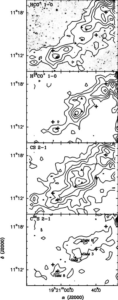
Figure 1: Contour maps of the integrated emission over the $v_{\rm LSR}$ range 6.05–8.45  km s^-1 of (from top to bottom) HCO⁺ (1$\rightarrow 0$), H¹³CO⁺ (1$\rightarrow 0$), CS (2$\rightarrow 1$), and C³⁴S (2$\rightarrow 1$). The HCO⁺ contour map is overlaid on the J band image from the 2MASS All-Sky Survey. The filled triangles show the submm sources reported by Visser, Richer & Chandler Visser02 (2002) (see labels in the bottom panel). The crosses show the positions of infrared sources from the IRAS Serendipitous Survey Catalog. From west to east: IRAS 19182+1112, IRAS 19183+1109, IRAS 19186+1106 and IRAS 19187+1107. Contour levels are 2, 3, 4, … 8 times 0.24 K  km s^-1for CS and HCO⁺ and 1, 2, 3, … 6 times 0.12 and 0.086 K  km s^-1 for C³⁴S and H¹³CO⁺, respectively.

The linear combination of the maps consists of first generating mosaicked BIMA dirty maps, $M_{\rm bima}$; as well as the BIMA dirty beam, $B_{\rm bima}$; then, the ”dirty” combined map and beam ($M_{\rm comb}$, $B_{\rm comb}$) are generated as follows (Stanimirovic et al. Stanimirovic99 (1999)):

$$M_{\rm comb}=\frac{M_{\rm bima}+f\,\alpha\,M_{\rm fcrao}}{1+\alpha}$$ (1)

$$B_{\rm comb}=\frac{B_{\rm bima}+\alpha\,B_{\rm fcrao}}{1+\alpha}$$ (2)

$M_{\rm fcrao}$ is the FCRAO map regridded to match the $M_{\rm bima}$ cell size and map size and weighted with the primary gain of the mosaicked BIMA maps; $B_{\rm fcrao}$ is modeled as a Gaussian with the FWHM given in Table 1; $f$ is the calibration factor, taken as 1.0 given the agreement of the relative flux calibration between the two instruments; and $\alpha$ is the ratio of the beam areas for the FCRAO and BIMA. We adopted a value of $\alpha=0.050$ and 0.042 for the CS and HCO⁺ data, respectively. The different $M_{\rm comb}$ were deconvolved from $B_{\rm comb}$ using the CLEAN algorithm. Note that modelling the FCRAO beam as a Gaussian is a good approximation: typical sidelobes in the beam pattern of a single-dish radio telescope are of the order of $-20$ dB, which will give an error in the combined beam pattern of less than $10^{-3}$, well below the dynamical range of the map.

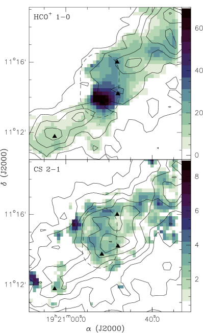
Figure 2: Grey scale image of the optical depth of HCO⁺ (1$\rightarrow 0$) (top panel) and CS (2$\rightarrow 1$) (bottom panel) derived from the integrated maps of Fig. 1. The scale levels are shown on the right side of each panel. The overlaid contour maps show the integrated emission of HCO⁺ and CS. The dashed line shows the gain at the 0.5 level of the BIMA primary beam response. The symbols are the same as those in Fig. 1.

As pointed out by Helfer et al. (Helfer03 (2003)), the method of adding synthetic single-dish visibilities in the $(u,v)$ plane is parameter-dependent, in particular on the number and weighting of the synthetic visibilities. Choosing the right combination of parameters, we found results almost identical to those of the linear method technique. Yet the linear method is much faster and simpler, so the combined maps presented here were obtained using the linear method. Details of the combined maps are shown in Table 2.

3 Results and Analysis

3.1 Spatial distribution of large scale molecular gas

Figure 1 shows the integrated emission maps of the four species observed with the FCRAO. The maps show that the high-density molecular emission arises from a filamentary structure oriented in the NW-SE direction. Despite sharing the same filamentary structure, the four maps show clear morphological differences. First, the CS is more spread out than HCO⁺: the FWHM along the axis perpendicular to the filament major axis is about $2^{\prime}$–$3^{\prime}$ for HCO⁺, whereas is about $3^{\prime}$–$5^{\prime}$ for CS. Second, the HCO⁺ and H¹³CO⁺ relative intensity peaks do not coincide. In particular, at the center of the map they are anti-correlated, i. e., the H¹³CO⁺ maximum is located in a relative minimum of the HCO⁺. Indeed the H¹³CO⁺ and HCO⁺ intensities are comparable at this position. This suggests a very high optical depth. In order to estimate quantitatively the effect of the opacity on the emission of CS and HCO⁺ we estimated their optical depths from the ratio of the integrated emission maps of H¹³CO⁺ and HCO⁺ and from C³⁴S and CS, using the isotope abundance ratios shown in Table 4. Figure 2 shows the grey scale image of the HCO⁺ and CS optical depth overlaid with the contour map of their integrated emission. This figure shows clearly that the HCO⁺ is highly optically thick, with $\tau\ga 7$ for most of the emitting region and with a maximum of $\tau=90$ at the position of L673 SMM 5. On the other hand, the CS emission is moderately optically thick ($\tau\simeq 1$–$4$).

Table 3: Selected positions

id.	Position		map counterpart a
	$\alpha$ (J2000)	$\delta$ (J2000)
a	19h20m34.3s	11∘18′05.5′′	IRAS 19182+1112
b	19h20m43.8s	11∘16′05.5′′
c	19h20m47.9s	11∘16′05.5′′	SMM 6
d	19h20m54.4s	11∘15′25.5′′	N
e	19h20m54.7s	11∘14′45.5′′
f	19h20m47.9s	11∘14′05.5′′	SMM 3
g	19h20m52.0s	11∘13′45.5′′	SMM 5 / S
h	19h21m02.9s	11∘11′45.5′′	SMM 8

• Positions N and S correspond to positions selected for study in MGE03.

The extremely high optical depths of the HCO⁺ (1$\rightarrow 0$) emission imply that this line is not a good tracer of the distribution of the HCO⁺ molecule in L673. Thus, we confirm the hypothesis pointed out by MGE03 that the high optical depth of HCO⁺ (1$\rightarrow 0$) is responsible for the lack of agreement between the observed BIMA HCO⁺ column densities and the theoretically predicted column densities. Indeed, the maximum HCO⁺ optical depth measured is located within the region observed with BIMA. Strong absorption features and very high optical depths of the HCO⁺ (1$\rightarrow 0$) emission are also observed in other molecular clouds (e. g., Langer et al. Langer78 (1978); Girart et al. Girart00 (2000)).

Table 4: Physical parameters

id.	$T_{\rm mb}$	$T_{\rm mb}$	$V^{a}$	$\Delta V^{b}$	Area	$\tau$c	$N^{d}$
	(CS)	(C34S)	(CS)	(CS)	(CS)	(CS)	(CS)
	(K)	(K)	(km s-1)	(km s-1)	(K km s-1)		(1013 cm-2)
a	1.34$\pm$0.14	$<0.14^{e}$	+7.0	0.7	$1.03\pm 0.06$	$<1.72$	0.95$-$1.53f
b	1.64$\pm$0.16	$0.32\pm 0.06$	+7.2	0.8	$1.48\pm 0.06$	4.21	$3.60\pm 0.14$
c	1.55$\pm$0.17	$0.26\pm 0.04$	+7.2	0.8	$1.31\pm 0.05$	3.61	$2.89\pm 0.10$
d	1.45$\pm$0.18	$0.24\pm 0.06$	+7.4	0.9	$1.37\pm 0.05$	3.53	$2.97\pm 0.10$
e	1.14$\pm$0.13	$0.19\pm 0.06$	+7.5	1.1	$1.38\pm 0.09$	3.48	$2.97\pm 0.19$
f	1.74$\pm$0.21	$0.32\pm 0.05$	+7.2	0.9	$1.66\pm 0.06$	3.99	$3.89\pm 0.15$
g	1.58$\pm$0.27	$0.35\pm 0.06$	+7.2	0.8	$1.38\pm 0.06$	5.04	$3.81\pm 0.17$
h	1.70$\pm$0.16	$0.19\pm 0.06$	+7.2	0.5	$0.98\pm 0.05$	2.04	$1.56\pm 0.07$
id.	$T_{\rm mb}$	$T_{\rm mb}$	$V^{a}$	$\Delta V^{b}$	Area	$\tau^{g}$	$N^{d}$	$N$
	(HCO+)	(H13CO+)	(H13CO+)	(H13CO+)	(H13CO+)	(H13CO+)	(H13CO+)	(HCO+)
	(K)	(K)	(km s-1)	(km s-1)	(K km s-1)		(1011 cm-2)	(1013 cm-2)
a	$1.49\pm 0.23$	$0.46\pm 0.12$	+7.0	0.4	$0.22\pm 0.03$	0.37	$3.86\pm 0.59$	$2.40\pm 0.36$
b	$1.53\pm 0.19$	$0.42\pm 0.06$	+7.1	0.5	$0.23\pm 0.03$	0.32	$3.91\pm 0.44$	$2.42\pm 0.27$
c	$0.95\pm 0.18$	$0.49\pm 0.07$	+7.2	0.7	$0.37\pm 0.02$	0.73	$7.16\pm 0.47$	$4.44\pm 0.29$
d	$0.70\pm 0.16$	$0.34\pm 0.05$	+7.4	0.7	$0.25\pm 0.03$	0.66	$4.77\pm 0.48$	$2.95\pm 0.30$
e	$0.54\pm 0.15$	$0.21\pm 0.07$	+7.5	0.5	$0.12\pm 0.02$	0.48	$2.12\pm 0.38$	$1.31\pm 0.24$
f	$1.17\pm 0.19$	$0.78\pm 0.04$	+7.3	0.5	$0.38\pm 0.02$	1.10	$8.12\pm 0.43$	$5.03\pm 0.26$
g	$0.81\pm 0.17$	$0.89\pm 0.05$	+7.3	0.5	$0.45\pm 0.02$	$>4^{h}$	$>18.2\pm 0.83$	$>11.3\pm 0.51$
h	$2.80\pm 0.25$	$0.42\pm 0.97$	+7.4	0.6	$0.25\pm 0.03$	0.16	$4.10\pm 0.48$	$2.55\pm 0.30$

• The error in the line velocity is lower than 0.1 km s^-1.

• The error in the line width is lower than 0.1 km s^-1.

• Using an abundance ratio CS/C³⁴S=20 and $T_{\rm ex}=4$ K.

• Beam averaged column density calculated from the formula in Table 3 of MGE03.

• Upper limit taken as $3\sigma$, where $\sigma$ is the sensitivity per channel.

• Range of values for $\tau\ll 1$ and $\tau=1.72$.

• using an abundance ratio HCO⁺/H¹³CO${}^{+}=62$ (Langer & Penzias Langer93 (1993)) and $T_{\rm ex}=4$ K.

• We adopt a value of $\tau=4$ as a lower limit.

From an inspection to the IRAS catalogues within the region shown in Fig. 1 we found four infrared sources. IRAS 19182+1112 and IRAS 19183+1109 are detected only at 12 and 25 $\mu$m. On the other hand, the other two sources, IRAS 19186+1106 and IRAS 19187+1107 are detected only at 100 $\mu$m. There are also four weak submillimeter sources (Visser, Richer & Chandler Visser02 (2002)). Only the strongest submm source, L673 SMM8, is associated with an infrared source, IRAS 19187+1107. All the submm sources are located in strong-molecular-line-emitting regions. Indeed, they are well correlated with the relative intensity peaks of H¹³CO⁺ (1$\rightarrow 0$). Visser et al. (Visser02 (2002)) classify these submm sources, except SMM3, as starless cores. SMM3 is classified as a candidate protostar (where there is some evidence of high-velocity CO emission).

By analyzing the kinematical properties of the CS and H¹³CO⁺ emission, we found a smooth velocity gradient along the major axis of the filamentary molecular structure: from NW to SE the $v_{\rm LSR}$ goes from $\sim 7.0$ to $7.4$  km s^-1. In addition, east of the center of the map the CS emission is redshifted to $\sim 7.7$ km s^-1.

3.1.1 Comparison of the emission of the CS (1$\rightarrow 0$) and (2$\rightarrow 1$) lines

We have also compared the CS (1$\rightarrow 0$) line measured with the Yebes telescope (Morata et al. Morata97 (1997)) with the CS (2$\rightarrow 1$) line obtained with the FCRAO telescope, after convolving the spectra of the (2$\rightarrow 1$) line with the 1.9^′ beam of the Yebes telescope. We compared the resulting spectra at the position of the CS (1$\rightarrow 0$) peak, corresponding to the North field of the BIMA map, and the position of the peak NH₃ intensity, corresponding to the South field. The derived $T_{\rm ex}$ at the North position is the same for both lines, 4.2 K. In the South position, where we did not observe the C³⁴S (1$\rightarrow 0$) transition, the excitation temperature derived from the (2$\rightarrow 1$) line, 4.4 K, is very similar to the value found in the northern region.

3.1.2 Column densities

As in MGE03, we selected several positions in the region mapped with the FCRAO observations in order to obtain the physical parameters of the gas and to compare them with the chemical model. Table 3 shows the coordinates for each position and their map counterparts, if any. These positions were selected mainly to coincide with the 4 positions we selected in MGE03, and with the SMM and IRAS sources of the region. We also selected two positions not related to any object in order to see if they traced “younger” gas. Table 4 shows the line parameters for the CS (2$\rightarrow 1$) and H¹³CO⁺ lines, and the physical parameters obtained for each position. We adopted a value of $T_{\rm ex}=4$ K for our calculations, based on the result we had obtained from the comparison between the CS (1$\rightarrow 0$) and (2$\rightarrow 1$) lines (Morata et al. Morata97 (1997) and MGE03, respectively).

Table 5: Ratio of column densities

id.	$N$(HCO+)/$N$(CS)
a	1.6–2.5a
b	$0.67\pm 0.08$
c	$1.54\pm 0.11$
d	$0.99\pm 0.10$
e	$0.44\pm 0.08$
f	$1.29\pm 0.08$
g	$>2.96\pm 0.19$
h	$1.63\pm 0.21$

• The value 1.6 is obtained for $\tau=1.72$. The value 2.5 is obtained when $\tau\ll 1$.

Table 5 shows the ratio between the derived column densities for CS and HCO⁺ obtained for each position, which can be compared to the results of our chemical model (MGE03). We observe that there is a similar trend to the results we obtained in MGE03. In the positions where there are no SMM or IRAS sources (positions b, d, and e) the CS column density is higher than the HCO⁺ column density, which would indicate that the clumps are chemically young. In the positions where there is a SMM or IRAS source, the column density fo HCO⁺ is higher than for CS. This is what we expect for later times, when the clumps are more chemically evolved, HCO⁺ is more abundant, and CS starts to suffer freeze-out. We found the highest ratio for SMM5 (position g), which we previously classified with the BIMA observations as one of the two chemically more evolved points, and where the N₂H⁺ emission is more intense. Thus, we confirm our previous classification.

3.1.3 CS abundances

Visser et al. (Visser02 (2002)) calculate the masses of the SMM sources in L673 from the total flux measured in an area of radius $r$. They also calculated the H₂ column density over this area. We have convolved the spectra of the CS (2$\rightarrow 1$) and C³⁴S (2$\rightarrow 1$) emission with a Gaussian with FWHM equal to the $r$ derived for each SMM source, in order to estimate the CS column density for each SMM position. Table 6 shows the averaged CS abundance obtained from the H₂ and CS column densities. The derived values are in the range 2–$10\times 10^{-9}$  cm^-2. We found the lowest value near the IRAS source at the SE part of the large scale maps, and the highest abundance at the position of SMM6, a submm source that seems to be less centrally peaked than other submm sources (Visser et al. Visser02 (2002)), which would indicate that it is in a less evolved stage.

Table 6: Calculated CS abundances at the positions of the SMM sources

	Beam	$\!\!\!\!\!\!N$(H2)a			$N$(CS)
	(arcsec)	(cm-2)	$\!\!\!\!\!T_{\rm C^{34}S}/T_{\rm CS}$	$\!\!\!\!\!\!\tau$	(cm-2)	$\!\!\!\!X$(CS)
SMM3	60	4.3$\times 10^{21}$	0.15$\pm 0.02$	3.2	2.74$\times 10^{13}$	6.4$\times 10^{-9}$
SMM5	80	4.0$\times 10^{21}$	0.18$\pm 0.02$	3.8	2.66$\times 10^{13}$	6.7$\times 10^{-9}$
SMM6	100	2.5$\times 10^{21}$	0.15$\pm 0.02$	3.2	2.56$\times 10^{13}$	1.0$\times 10^{-8}$
SMM8	110	3.8$\times 10^{21}$	0.11$\pm 0.02$	2.0	1.08$\times 10^{13}$	2.8$\times 10^{-9}$

3.2 Spatial distribution at high angular resolution

Figure 3 shows the composite of the combination process of the BIMA and FCRAO observations for the CS (2$\rightarrow 1$) and HCO⁺ (1$\rightarrow 0$) emission.

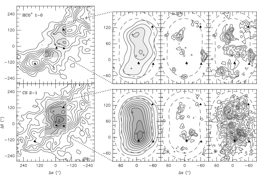
Figure 3: Composite of the combination process for CS (2$\rightarrow 1$) (bottom panels) and HCO⁺ (1$\rightarrow 0$) (top panels). All maps show the integrated emission over the $v_{\rm LSR}$ range 6.05–8.45  km s^-1. Left panels: FCRAO maps. Middle-left panels: FCRAO maps corrected for the primary beam of the mosaicked BIMA maps. Middle-right panels: mosaicked BIMA maps. Right panels: Combined BIMA and FCRAO maps. For the FCRAO maps, the contour levels are 3, 4, 5, … 12 times 3.17 and 2.80 Jy beam^-1 km s^-1 for CS (2$\rightarrow 1$) and HCO⁺ (1$\rightarrow 0$), respectively. For the BIMA and combined maps, the contour levels are 2, 3, 4, … 9 times 0.27 and 0.24 Jy beam^-1 km s^-1 for CS (2$\rightarrow 1$) and HCO⁺ (1$\rightarrow 0$), respectively. The inner and outer dashed lines show the 0.5 and 0.25 level of the BIMA primary beam response. The symbols are the same as those in Fig. 1.

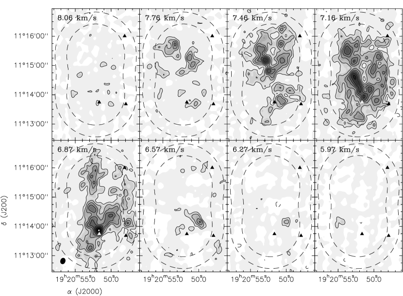
Figure 4: Channel maps of the CS (2$\rightarrow 1$) emission. The contour levels are -3, 3, 4.5, 6, … 12 times 0.24 Jy beam^-1 (the rms noise of the maps). The inner and outer dashed lines show the 0.5 and 0.25 level of the BIMA primary beam response. The symbols are the same as in Fig. 1.

The HCO⁺ combined map shows a clear filamentary structure connecting several clumps, although some of them, particularly to the SE, are far from the phase center of the map, which makes it difficult to distinguish them from another filament. However, as indicated by Fig. 2, the region observed has a very high optical depth, so the emission shown in the combined map cannot be used to describe the true morphological and kinematical behaviour of the HCO⁺ emission.

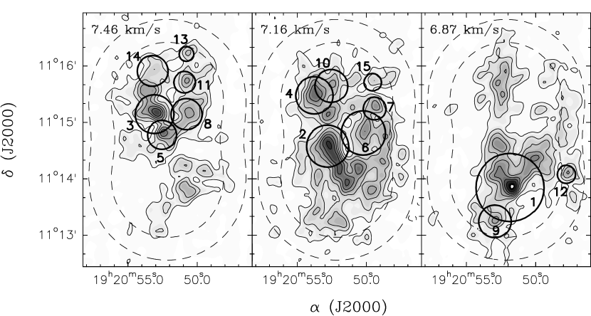
Figure 5: Combined BIMA and FCRAO CS (2$\rightarrow 1$) contour maps for the three channels with the strongest emission (from Fig. 4). The thick circles are centered at the position and at the channel at which each clump shows its highest intensity, as found by the CLFIND algorithm of Williams et al. (Williams94 (1994)) and described in Sect. 3.3. The areas of the circles are proportional to the masses of the clumps. The numbers correspond to the identifier in the first column of Table 7.

On the other hand, the combined map of the CS emission, although it has a moderately high opacity (2–4), can be used to trace the CS distribution. When we recover all the flux, we find that all the most prominent clumps found in the BIMA observations are also detected but with more intensity. We believe that these clumps, which lie near the phase center of the map, are real. We also recover emission from a great deal of other structure which was not, or only marginally, detected previously. This confirms the predicted effect of the BIMA filtering in MGE03. The overall aspect is also of a filamentary structure connecting several intense clumps. One of these clumps coincides with the nominal position of the source SMM 5.

The clumps and the filamentary structure of the emission are more clearly revealed in Fig. 4, which shows the channel maps of the combined BIMA and FCRAO maps for the CS (2$\rightarrow 1$) line. Here we find a very complex structure, with several clumps with sizes of $\sim 13^{\prime\prime}$–$25^{\prime\prime}$, appearing in two or three of the channel maps. Some of these clumps might coincide with clumps found in the HCO⁺ map.

3.3 Clump Analysis

Since the combined high-angular-resolution maps show a highly clumpy CS spatial and velocity structure, we carried out the clump analysis technique developed by Williams, de Geus & Blitz (Williams94 (1994)) in our combined BIMA and FCRAO CS (2$\rightarrow 1$) data cube. This technique consists mainly of two algorithms, CLFIND and CLSTATS. CLFIND, which does not assume any clump profile, works by contouring the data at a multiple of the rms noise of the data cube, then searches for peaks of emission to locate the clumps, and then follows them down to lower intensities. CLSTATS is a task that calculates integrated intensities, peak positions, sizes, velocity dispersion, etc, for the clumps found by CLFIND. A very detailed explanation of this analysis technique is found in Williams et al. (Williams94 (1994)), who also found that the CLFIND algorithm obtains the best results when the contour interval and the lower contour are set to 2$\sigma$. However, they recommend using a higher value of the lower contour if there is background emission. This is the case for the combined L673 CS (2$\rightarrow 1$) maps, where there is some low-level ($\sim 2\sigma$) extended emission. Thus, we run the CLFIND and CLSTATS algorithms for the L673 CS channel maps with the contour interval set to 0.48  Jy beam^-1 (2$\sigma$) and the lowest contour set at 0.96  Jy beam^-1 (4$\sigma$).

Table 7: Clumps within the BIMA primary beam

N $$\!\!\!T_{\rm peak}$$ (H

(K) (km s^-1) (pc) () () cm^-3)

1 3.5 3.2 0.49 0.045 0.36 2.28 1.9

2 3.0 3.2 0.39 0.037 0.14 1.18 1.3

3 2.8 2.7 0.43 0.023 0.12 0.89 4.6

4 2.5 2.8 0.55 0.026 0.11 1.65 3.0

5 2.5 2.7 0.51 0.020 0.07 1.08 4.1

6 2.2 3.1 0.38 0.036 0.15 1.10 1.6

7 2.1 2.6 0.37 0.025 0.04 0.73 1.2

8 2.0 3.5 0.49 0.022 0.08 1.12 3.4

9 2.0 2.4 0.31 0.033 0.08 0.64 1.2

10 2.0 3.0 0.56 0.021 0.09 1.39 4.4

11 1.9 2.7 0.44 0.020 0.04 0.80 2.3

12 1.9 1.9 0.57 0.027 0.03 1.83 0.6

13 1.6 4.0 0.39 0.015 0.02 0.47 2.5

14 1.4 3.0 0.65 0.022 0.07 1.98 3.3

15 1.4 2.0 0.39 0.021 0.02 0.67 1.2

• Optical depth derived at the peak position of the clump from the intensity ratio of the CS (2$\rightarrow 1$) and C³⁴S (2$\rightarrow 1$) FCRAO maps.

• FWHM of the line corrected for channel resolution as described in Appendix A of Williams et al. (1994)

• Equivalent circular radius corrected for beam size as described in Appendix A of Williams et al. (1994)

• Clump mass derived from the integrated emission obtained with CLSTATS corrected for the CS (2$\rightarrow 1$) optical depth, $\tau$, and assuming a constant excitation temperature of $T_{ex}=4$ K. An abundance ratio of $X[{\rm CS/H}_{2}]=10^{-8}$ is adopted.

• Virial mass obtained from $M_{\rm vir}=5\,\Delta R\,\sigma_{v}^{2}/\alpha\,G$ with $\sigma_{v}=\Delta v/2.355$ and assuming an inverse-square power law density profile ($\alpha$=5/3).

• Average volume density obtained assuming a sphere of mass $M_{\rm cl}$ and radius $\Delta R$.

A total of 15 clumps were found, all of them with a peak intensity of at least $\sim 4\sigma$. Table 7 lists the physical parameters derived for the 15 clumps found by the algorithm. All the clumps are clearly resolved at our angular resolution, and have deconvolved diameters in the 0.03–0.09 pc range. The velocity dispersion of the clumps (i. e., the FWHM corrected for the spectral resolution) is not very different for the different clumps, 0.31–0.65  km s^-1. The clumps have masses between 0.02 and 0.36 $M_{\sun}$. The estimated clump densities range between 0.6 and $4.6\times 10^{4}$  cm^-3. This value of the averaged density of the clumps implies that, since the CS (2$\rightarrow 1$) critical density is $5\times 10^{5}$  cm^-3, they are subthermalized. It also explains why the derived excitation temperature, 4 K, is significantly below the kinetic temperature expected in the cloud, 10 K.

Figure 5 shows the location of the clumps derived by the algorithm as circles. The areas of the circles are proportional to the masses of the clumps. This figure shows a segregation of clumps between the northern and southern section of the map. The clumps with peak intensities in the 7.2 and 7.5  km s^-1 channels arise from the northern region, whereas the clumps that have a peak in the 6.9  km s^-1 channel are located in the southern region. In addition, the southern part contains fewer clumps than the northern part, but it is dominated by the largest and most massive clump. Interestingly, this clump is associated with the two N₂H⁺ clumps found by MGE03. This confirms the idea that both N₂H⁺ and NH₃ trace the more evolved, massive clumps.

4 Discussion

4.1 The large-scale structure of L673. Correlation of HCO⁺ and N₂H⁺ emission with dust

As we have pointed out, the H¹³CO⁺ seems to be well correlated with the dust as detected by the submillimeter observations. This suggests that H¹³CO⁺ traces the more massive or more evolved clumps. At the same time, Fig 1 shows that the peak H¹³CO⁺ emission is also coincident with the position of the BIMA peak of N₂H⁺, and a SMM source (SMM 5). In our chemical models, HCO⁺ and N₂H⁺ are late-time molecules. Thus, the apparent discrepancy found in MGE03 between the column densities observed with BIMA and the expected values from the chemical model was due to the extremely high opacity of the HCO⁺ emission. H¹³CO⁺ is found where N₂H⁺ is also found, although a little more extended, as can be expected from the models, because it is formed a little earlier. Moreover, the emission of H¹³CO⁺, a late-time molecule, coincides with the position of the dusty submm sources, which also agrees with the theoretical predictions (Taylor et al. Taylor98 (1998)).

4.2 The small-scale structure of L673

4.2.1 CS clump distribution properties

Figure 6 shows the mass and size distribution of the derived clumps. It is clear that with only 15 clumps we cannot pursue a statistical analysis of the mass distribution of the clumps. However, with the data available, the mass clump distribution is compatible with the low-mass end of the mass distribution observed in low-mass star formation clouds, such as in $\rho$ Oph (Motte et al. Motte98 (1998); Johnstone et al. Johnstone00 (2000)), where the slope of $dN/dM$ is not so steep (see Fig. 6).

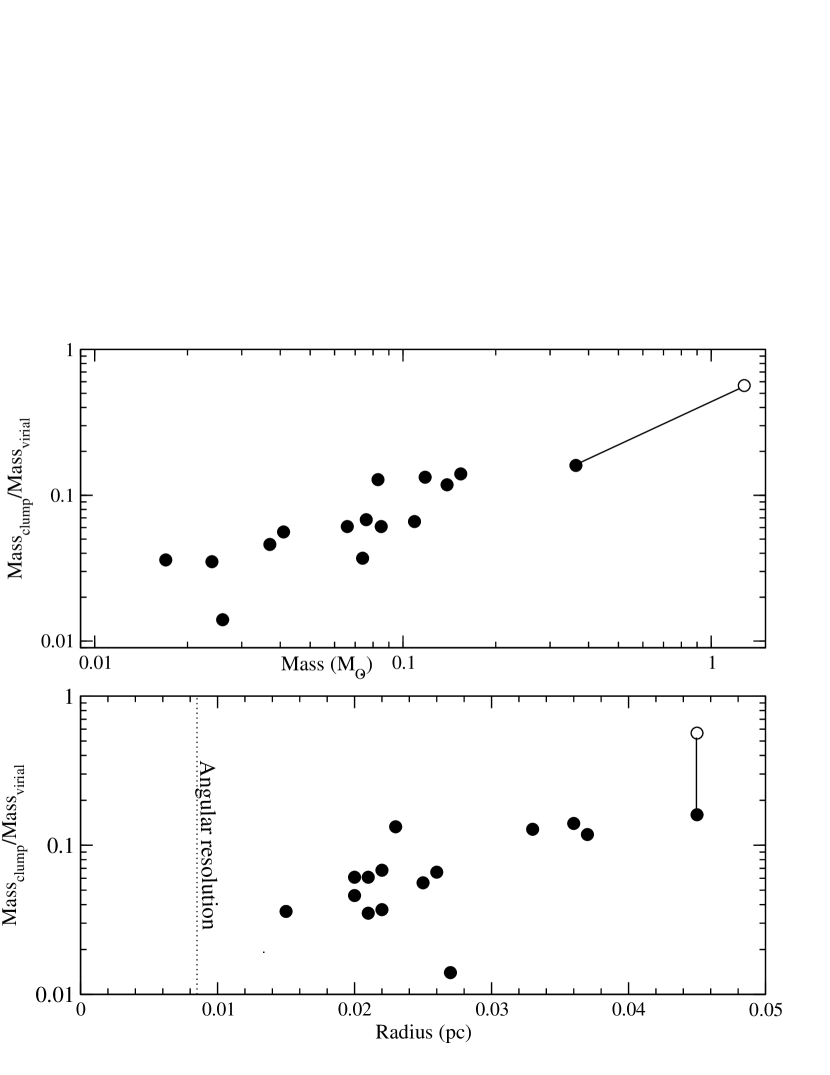
Figure 7: Relation between the clump to virial mass ratio with respect to the clump mass (top) and the equivalent circular radius (bottom). The open circle represents the most massive clump when the mass derived from the N₂H⁺ emission is considered.

The derived clump masses are significantly below the virial mass (see Table 7). This strongly supports the idea that these clumps must be transient (Taylor et al. Taylor96 (1996), Taylor98 (1998)). Recently, a detailed study of the illuminated clumps ahead of the HH 2 object also suggested that clumps in molecular clouds are transient (Girart et al. Girart02 (2002); Viti et al. Viti03 (2003)). Fig. 7 also shows that the mass of the clumps becomes closer to the virial mass when they get bigger and more massive, which is when they have a higher chance to form stars. However, the mass calculated for the clumps is derived assuming constant CS abundance. If, as it seems, the CS abundance is lower for more evolved clumps, the slope of the relation shown in Fig. 7 would be steeper, and the clumps would probably have a mass closer to the virial mass.

4.2.2 Largest clump and N₂H⁺ clumps properties

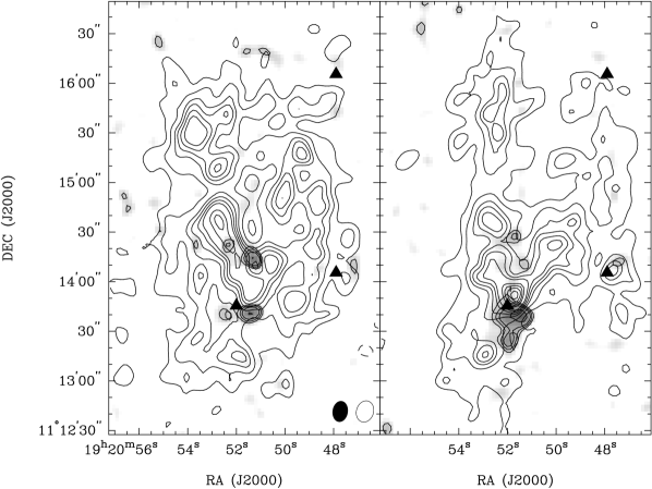
Figure 8: Comparison of the channel maps of the combined CS (2$\rightarrow 1$) emission (solid contours) for the 7.16 (left) and 6.87 km s^-1 (right) channels; and the BIMA N₂H⁺ (1$\rightarrow 0$) emission (contours and grey scale) for the $-0.8$ (left) and $-1.1$ km s^-1 (right) channels. The contour levels for the CS maps are the same as in Fig. 4. The contour levels for the N₂H⁺ maps are 3, 3.5, 4, 5, 6, and 7 times 0.20 Jy beam^-1 (the rms noise of the maps). The symbols are the same as those in Fig. 1.

Figure 8 shows the comparison of two channel maps for the combined CS (1$\rightarrow 2$) and N₂H⁺ (1$\rightarrow 0$) emission. We can clearly see that the peak of the CS emission is shifted with respect to the peak of N₂H⁺. Moreover, the CS emission is more spread than N₂H⁺, so we are detecting chemical differentiation inside the clump.

The largest CS clump is not only the clump with the highest $M_{\rm clump}/M_{\rm virial}$ ratio (and thus with the highest probability of undergoing star formation) but it is also the only one associated with N₂H⁺ emission (see Sect. 3.3). This confirms the Taylor et al. (Taylor96 (1996), Taylor98 (1998)) scenario. Interestingly, the density of this clump, as derived from the CS emission, is similar to that of the other clumps. This may be explained if the emission of the N₂H⁺ traces the highest densities of the clump, high enough for CS depletion to occur, as has been observed in several dense starless cores (e. g., Tafalla et al. Tafalla02 (2002), Tafalla04 (2004)).

We have calculated from the BIMA data the mass traced by the N₂H⁺ for this clump. Assuming a N₂H⁺ fractional abundance of $8\times 10^{-11}$, which was obtained using the H₂ column density determination from the submm sources of Visser et al. (Visser02 (2002)), we could derive a total mass for the biggest clump of 1.2 $M_{\sun}$. This mass is significantly higher than those of the other clumps. In addition, $M_{\rm clump}/M_{\rm vir}$ is 0.52, so it is close to collapse.

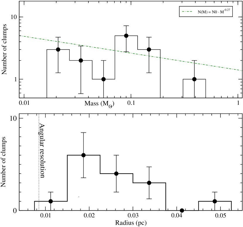
Figure 6: Top Mass distribution of the L673 CS clumps within the primary beam of the BIMA maps. The lines show the clump mass spectrum for a power-law distribution, $N\propto M^{-0.27}$. Bottom Size (equivalent circular radius) distribution of the L673 CS clumps. The dotted line shows the radius of the CS (2$\rightarrow 1$) synthesized beam. Note that all the clumps are well resolved at our angular resolution.

4.2.3 On the small scale structure of L673

The previous results, along with the results from the lower-resolution analysis in Sect. 3.1.2, show at least the differences between the two regions within the BIMA observations. The northern region shows a gas less chemically evolved, and smaller and more numerous clumps. The southern region contains the more evolved gas and the biggest clump.

The clumps detected in our observations seem to be of a different kind than the ones usually studied in surveys of “starless cores” (Tafalla et al. Tafalla02 (2002); Bergin et al. Bergin01 (2001)). Those are usually older cores, which have already achieved the more evolved and more massive stage of evolution, as is clearly indicated by the detection of late-time molecules, as N₂H⁺ and NH₃, and by the high level of depletion of some molecules onto dust grains. We find one such clump in our region, which might be just arriving at that evolved phase. This clump is at the same time the most massive, shows emission of N₂H⁺, and different emission peaks for CS and N₂H⁺, which could point to depletion. However, we detect many other clumps, less massive, that show almost no emission of late-time molecules, and which probably will disperse before they can achieve the “starless core” stage.

We face the question of what the origin of these transient clumps could be. They are probably caused by interstellar turbulence (see e.g. Padoan Padoan95 (1995); Ballesteros-Paredes et al. Ballesteros99 (1999)). In support of this idea, we observe that the derived masses for our clumps are around 0.1$M_{\sun}$, which is also the mass-scale of turbulent fragmentation in the ISM (Padoan Padoan95 (1995)). This small scale turbulence is probably related to large-scale flows in the diffuse Galactic interstellar medium, which several studies (Hartmann et al. Hartmann01 (2001); Bergin et al. Bergin04 (2004)) propose as a mechanism that can lead to the fast formation and dispersal of molecular clouds, which could explain the apparent rapid star formation and short cloud lifetimes observed in the regions of the solar neighborhood. On a smaller scale, several authors postulate the possible existence of transient clumps. Falle & Hartquist (Falle02 (2002)) propose that slow-mode MHD waves could create, under suitable conditions, large density enhancements, of the order of a factor of 30, which could last on the order of 1 Myr, before dispersing back to the original density. At the same time, Vázquez-Semadeni et al. (Vazquez-ph (2005), Vazquez03 (2003)) and Ballesteros-Paredes et al. (Ballesteros03 (2003)) also argue that cores within molecular clouds may not be in hydrostatical equilibrium, and would be transient features generated by the dynamical flow in the cloud, not necessarily requiring strong magnetic fields. These cores must then either collapse, if they have an excess of gravitational energy, or re-expand and merge back into the surrounding molecular cloud. The re-expansion time is expected to be longer than the compression time because of the retarding action of self-gravity, and is estimated to be of the order of a few free-fall times. This would be consistent with the result that typically there are more starless than star-forming cores in molecular clouds and that, as in our case, most of the cores do not appear to be gravitationally bound. Only sufficiently massive cores would eventually undergo local collapse.

In any case, such models would have consequences for the physical and chemical evolution of these regions (Williams & Viti Williams02 (2002)). Firstly, the chemistry would be mainly “young”, as the molecules would be destroyed when the gas returns to a more diffuse state. Secondly, this mechanism would halt the process of freeze-out of molecules onto dust, as the frozen-out molecules would also return to the gas phase as the density of the gas goes back to the diffuse state. Thus, these regions would not be completely depleted of molecules in the gas phase, as is apparently shown by some observations (Gibb & Little Gibb98 (1998)). Finally, the mass distribution of these transient clumps probably determines the low-mass star formation rate.

However, an alternative possibility is that the more massive clumps were formed by aggregation of smaller clumps into a massive one, which could then be closer to collapse. The analysis of our clumps allows us to make some rough estimates to see if this can happen since transient clumps are expected to survive for $\sim 1$ Myr (Falle & Harquist 2002; Vázquez-Semadeni et al. 2004). Two limiting cases can be studied. One is that of a 1-dimensional structure, that is, the clumps are assumed to move inside a filamentary structure, with relative velocities (between clumps) of $0.3$ km s^-1. This is the typical difference in the radial velocities of the clumps, which should roughly give a reasonable lower limit for the true relative velocities. In the course of $\sim 1$ Myr any of the observed clumps would have travelled $\sim 63000$ AU or $\sim 3\aas@@fstack{\prime}5$, which is the size of the field of view of our maps. The other case is that of a 3-dimensional (3-D) structure with similar scales in the three dimensions. In this case the projected area of this volume in any particular direction is $A_{\rm proj}\simeq V_{\rm tot}^{2/3}$, where $A_{\rm proj}$ and $V_{\rm tot}$ are the area and volume, respectively. Let us assume that in a volume $V_{\rm tot}$ there are $n$ identical spherical clumps of radius $R$ distributed randomly, with a random velocity distribution with an average velocity $\langle v_{\rm 3D}\rangle$. The 3-D filling factor of the clumps for this volume is $f_{\rm 3D}=nV_{\rm cl}/V_{\rm tot}=nV_{\rm cl}/A_{\rm proj}^{3/2}$, where $V_{\rm cl}$ is the clump volume. The volume swept up by a clump in a time $t$ is $V_{\rm sw}(t)=v_{\rm 3D}\,t\,\pi R^{2}$. For a given clump, the time scale needed to cross another clump, $t_{X}$, is such that $f_{\rm 3D}\,V_{\rm sw}(t_{X})=V_{\rm cl}$. From the previous equations, the average crossing scale time can be written as $\langle t_{X}\rangle=A_{\rm proj}^{3/2}/(n\,\langle v_{\rm 3D}\rangle\,\pi R^{2})$. Since what we measure is the radial velocity, $v_{\rm obs}$ and $\langle v_{\rm 3D}\rangle=2\,\langle v_{\rm obs}\rangle$, then $\langle t_{X}\rangle=A_{\rm proj}^{3/2}/(2\,n\,\langle v_{\rm obs}\rangle\,\pi R^{2})$. For $A_{\rm proj}$ equal to our field of view ($\sim 3\aas@@fstack{\prime}5\times 2\aas@@fstack{\prime}0$), which includes 15 clumps, and using a radius equal to the average value for the measured clumps (from Table 7), $R\simeq 18^{\prime\prime}$, we found that $\langle t_{X}\rangle\simeq 6\times 10^{5}$ yr. Then it could be possible that star formation was the result not of the gravitational collapse of just one clump, but of a “merging” effect. In this case, the geometry of dense cores would be far from spherical symmetry, even the density distribution would not follow $n(r)\propto r^{-2}$. Tafalla et al. (Tafalla04 (2004)) find that their starless cores are not spherical, but that clear inhomogeneities are found in them.

5 Conclusions

We have made a multitransitional study of the spatial distribution of the molecular emission with the 14 m FCRAO telescope in the starless core found in the L673 region, which had been previously observed at lower angular resolution (Morata et al. Morata97 (1997)) and with the BIMA array (MGE03). The main goal of these observations was to combine them with the array observations in order to obtain high resolution maps of the full emission, and thus be able to confirm that the clumpy structure detected with the BIMA telescope was real. The main results were:

1. With the FCRAO we detected emission in the CS (2$\rightarrow 1$), C³⁴S (2$\rightarrow 1$), HCO⁺ (1$\rightarrow 0$), and H¹³CO⁺ (1$\rightarrow 0$) lines. Although every map shows clear morphological differences, we found that the high density molecular emission in the four molecules arises from a filamentary structure oriented in the NW-SE direction. The ratio between HCO⁺ and H¹³CO⁺ also confirms that the apparent lack of HCO⁺ (1$\rightarrow 0$) emission in the BIMA maps was due to the extremely high optical depth in this line. We also found that several submm sources detected in this region are located in strong molecular line emitting regions, and that they seem to be well correlated with the relative intensity peaks of H¹³CO⁺.

2. We selected several positions to study the local physical parameters. We confirm the results of MGE03: the column density of CS is higher than that of HCO⁺ for positions were the gas is chemically younger, i.e. not associated with IRAS or submm sources. In the positions where there is a submm or IRAS source, the HCO⁺ column density is higher than that of CS.

3. The BIMA and FCRAO combined maps of the CS emission show that all the prominent clumps found in the BIMA observations are also detected but with more intensity. We believe that these clumps are real. We also recover emission from other structure which was previously undetected or only marginally detected. The overall aspect is also of a filamentary structure connecting several intense clumps.

4. We found a total of 15 clumps in our combined data cube. All of them are resolved at our angular resolution, with diameters in the 0.03$-$0.09 pc range. Their estimated masses range between 0.02 and 0.36 $M_{\sun}$, and their densities between 0.6 and 4.6$\times 10^{4}$ cm^-3, which indicates that the CS (2$\rightarrow 1$) emission is clearly subthermalized.

5. There is a clear segregation in the properties of the detected clumps between the northern and southern regions of the map. The northern region shows the less chemically evolved gas, and less massive but more numerous clumps. On the other hand, the southern region contains the more evolved gas and the most massive clump. This clump is also the only one associated with BIMA N₂H⁺ emission. Moreover the H¹³CO⁺ emission correlates well with the dust emission traced by the submillimeter observations, and its emission peak also coincides with the BIMA N₂H⁺ peak and the SMM 5 source. All these results support the predictions of our chemical model, which proposed that late-time molecules, such as N₂H⁺ and HCO⁺, should be found in the same regions.

6. The clump masses derived are below the virial mass, which means that these clumps must be transient, as only the more massive ones are able to condense into stars.

7. The properties of the clumps we detect seem to be different from those of the “starless cores” recently found in the literature. Although we might have detected one such core, the rest are in an early evolutionary stage, after which they will most likely disperse.

We find that the simple chemical model proposed in MGE03 to explain the properties of the CS core of L673 is confirmed by the combination of single-dish and array observations. However, there is still a lot of work to be done on the formation mechanisms of these clumps and on the possibility that the merging of smaller clumps can lead to more massive and gravitationally unstable clumps. Further observing and modelling of the chemistry of these clumps and of the interclump gas will be needed in order to test the transient nature of the clumps.

- (1) Ballesteros-Paredes, J., Klessen, R. S., & Vázquez-Semadeni, E. 2003, ApJ, 592, 188
- (2) Ballesteros-Paredes, J., Vázquez-Semadeni, & E., and Scalo, J. 1999, ApJ, 515, 286
- (3) Bergin, E. A., Ciardi, D. R., Lada, C. J., Alves, J., & Lada, E. A. 2001, ApJ, 557, 209
- (4) Bergin, E. A., Hartmann, L. W., Raymod, J. C., Ballesteros-Paredes, J. 2004, ApJ, 612, 921
- (5) Falle, S. A. E. G., & Hartquist, T. W. 2002, MNRAS, 329, 195
- (6) Gibb, A. G., & Little, L. T. 1998, MNRAS, 295,299
- (7) Girart, J. M., Ho, P. T. P., Rudolph, A. L., Estalella, R., Wilner, D. J., & Chernin, L. M. 1999, ApJ, 522, 921
- (8) Girart, J. M., Estalella, R, Ho, P. T. P., & Rudolph, A. L. 2000, ApJ, 539, 763
- (9) Girart, J. M., Viti, S., Williams, D. A., Estalella, R, & Ho, P. T. P. 2002, A&A, 388, 1004
- (10) Hartmann, L. W., Ballesteros-Paredes, J., Bergin, E. A. 2001, ApJ, 562, 852
- (11) Helfer, T. T., Thornley, M. D., Regan, M. W., et al. 2003, ApJS, 145, 259
- (12) Herbig, G. H., & Jones, B. F. 1983, AJ, 88, 1040
- (13) Johnstone, D., Wilson, C. D., Moriarty-Schieven, G., et al. 2000, ApJ, 545, 327
- (14) Langer, W. D., Wilson, R. W., Henry, P. S., & Guélin, M. 1978, ApJ, 225, L139
- (15) Langer, W. D., & Penzias, A. 1993, ApJ, 408, 539
- (16) Morata, O., Estalella, R., López, R., & Planesas, P. 1997, MNRAS, 292, 120
- (17) Morata, O., Girart, J. M., & Estalella, R. 2003, A&A, 397, 181 (MGE03)
- (18) Motte, F., André, P., & Neri R. 1998, A&A, 336,150
- (19) Myers, P. C., Fuller, G. A., Goodman, A. A., & Benson, P. J. 1991, ApJ, 376, 561
- (20) Padoan, P. 1995, MNRAS, 277, 377
- (21) Pastor, J., Estalella, R., López, R., et al. 1991, A&A, 252, 320
- (22) Stanimirovic, S., Staveley-Smith, L., Dickey, J. M., Sault, R. J., & Snowden, S. 1999, MNRAS, 302, 417
- (23) Tafalla, M., Myers, P. C., Caselli, P., & Walmsley, C. M. 2004, A&A, 416, 191
- (24) Tafalla, M., Myers, P. C., Caselli, P., Walmsley, C. M., & Comito, C. 2002, ApJ, 569, 815
- (25) Taylor, S. D., Morata, O., & Williams, D. A. 1996, A&A, 313, 269
- (26) Taylor, S. D., Morata, O., & Williams, D. A. 1998, A&A, 336, 309
- (27) Vázquez-Semadeni, E., Ballesteros-Paredes, J., & Klessen, R. S. 2003, ApJ, 585, L131
- (28) Vázquez-Semadeni, E., Kim, J., Shadmehri M., & Ballesteros-Paredes, J. 2005, ApJ, 618, 344
- (29) Visser, A. E., Richer, J. S., & Chandler, C. J. 2002, AJ, 124, 2756
- (30) Viti, S., Girart, J. M., Garrod, R., Williams, D. A., & Estalella, R. 2003, A&A, 399, 187
- (31) Vogel, S. N., Wright, M. C. H., Plambeck, R. L., & Welch, W. J. 1984, ApJ, 283, 655
- (32) Williams, D. A., & Viti, S., 2002, in Chemistry as a Diagnostic of Star Formation, ed. C. L. Curry, & M. Fich (Ottawa, Canada: NRC Press), 106
- (33) Williams, J. P., de Geus, E. J., & Blitz, L. 1994, ApJ, 428, 693
- (34) Ye, T., Turtle, A. J., & Kennicutt, R. C. 1991, MNRAS, 249, 722
- (35) Zhou, S., Wu, Y., Evans, N. J., Fuller, G. A., & Myers, P. C. 1989, ApJ, 346, 168