When Supermassive Black Holes were growing: Clues from Deep X–ray Surveys

Abstract

Merging the Chandra and XMM–Newton deep surveys with the previously identified ROSAT surveys a unique sample of almost 1000 AGN–1 covering five orders of magnitude in 0.5–2 keV flux limit and six orders of magnitude in survey solid angle with $\sim 95\%$ completeness has been constructed. The luminosity–redshift diagram is almost homogeneously filled. AGN–1 are by far the largest contributors to the soft X–ray selected samples. Their evolution is responsible for the break in the total 0.5–2 keV source counts. The soft X–ray AGN–1 luminosity function shows a clear change of shape as a function of redshift, confirming earlier reports of luminosity–dependent density evolution for optical quasars and X–ray AGN. The space density evolution with redshift changes significantly for different luminosity classes, showing a strong positive evolution, i.e. a density increase at low redshifts up to a certain redshift and then a flattening. The redshift, at which the evolution peaks, changes considerably with X–ray luminosity, from $z\approx$0.5–0.7 for luminosities $\log L_{x}$=42–43 erg s^-1 to $z\approx 2$ for $\log L_{x}$=45–46 erg s^-1. The amount of density evolution from redshift zero to the maximum space density also depends strongly on X–ray luminosity, more than a factor of 100 at high luminosities, but less than a factor of 10 for low X–ray luminosities. For the first time, a significant decline of the space density of X–ray selected AGN towards high redshift has been detected in the range $\log L_{x}$=42–45 erg s^-1, while at higher luminosities the survey volume at high–redshift is still too small to obtain meaningful densities. A comparison between X–ray and optical properties shows now significant evolution of the X–ray to optical spectral index for AGN–1. The constraints from the AGN luminosity function and evolution in comparison with the mass function of massive dark remnants in local galaxies indicates, that the average supermassive black hole has built up its mass through efficient accretion ($\epsilon\sim 10\%$) and is likely rapidly spinning.

1 Introduction

In recent years the bulk of the extragalactic X–ray background in the 0.1-10 keV band has been resolved into discrete sources with the deepest ROSAT, Chandra and XMM–Newton observations has98 ; mus00 ; gia01 ; gia02 ; has01 ; ale03 ; wor04 ; bau04 . Optical identification programmes with Keck schm98 ; leh01 ; bar01a ; bar03 and VLT szo04 ; fio03 find predominantly unobscured AGN–1 at X–ray fluxes $S_{X}>10^{-14}$ erg cm^-2 s^-1, and a mixture of unobscured and obscured AGN–2 at fluxes $10^{-14}>S_{X}>10^{-15.5}$ erg cm^-2 s^-1 with ever fainter and redder optical counterparts, while at even lower X–ray fluxes a new population of star forming galaxies emerges hor00 ; ros02 ; ale02 ; hor03 ; nor04 ; bau04 . At optical magnitudes R$>$24 these surveys suffer from large spectroscopic incompleteness, but deep optical/NIR photometry can improve the identification completeness significantly, even for the faintest optical counterparts zhe04 ; mai04 . A recent review article bra05 summarizes the current status of X–ray deep surveys.

The AGN/QSO luminosity function and its evolution with cosmic time are key observational quantities for understanding the origin of and accretion history onto supermassive black holes, which are now believed to occupy the centers of most galaxies. X–ray surveys are practically the most efficient means of finding active galactic nuclei (AGNs) over a wide range of luminosity and redshift. Enormous efforts have been made by several groups to follow up X–ray sources with major optical telescopes around the globe, so that now we have fairly complete samples of X–ray selected AGNs. The most complete and sensitive sample was compiled recently by Hasinger, Miyaji and Schmidt has05 , concentrating on unabsorbed (type–1) AGN selected in the soft (0.5–2 keV) X–ray band, where due to the previous ROSAT work paper1 ; paper2 complete samples exist, with sensitivity limits varying over five orders of magnitude in flux, and survey solid angles ranging from the whole high galactic latitude sky to the deepest pencil-beam fields. These samples allowed to construct luminosity functions over cosmological timescales, with an unprecedented accuracy and parameter space.

Table 1: The soft X–ray sample

Surveya	Solid Angle	$S_{\rm X14,lim}$	$N_{\rm tot}$	$N_{\rm AGN-1}$b	$N_{\rm unid}^{\rm c}$
	[deg2]	[cgs]
RBS	20391	$\approx 250$	901	203	0
SA–N	684.0–36.0	47.4–13.0	380	134	5
NEPS	80.7–1.78	21.9–4.0	262	101	9
RIXOS	19.5–15.0	10.2–3.0	340	194	14
RMS	0.74–0.32	1.0–0.5	124	84	7
RDS/XMM	0.126–0.087	0.38–0.13	81	48	8
CDF–S	0.087–0.023	0.022–0.0053	293	113	1
CDF–N	0.048–0.0064	0.030–0.0046	195	67	21
Total			2566	944	57

^a Abbreviations – RBS: The ROSAT Bright Survey schw00 ; SA–N: ROSAT Selected Areas North app98 ; NEPS: ROSAT North Ecliptic Pole Survey gio03 ; RIXOS: ROSAT International X–ray Optical Survey mas00 , RMS: ROSAT Medium Deep Survey, consisting of deep PSPC pointings at the North Ecliptic Pole bow96 , the UK Deep Survey mch98 , the Marano field zam99 and the outer parts of the Lockman Hole schm98 ; leh00 ; RDS/XMM: ROSAT Deep Survey in the central part of the Lockman Hole, observed with XMM–Newton leh01 ; mai02 ; fad02 ; CDF–S: The Chandra Deep Field South szo04 ; zhe04 ; mai04 ; CDF–N: The Chandra Deep Field North bar01a ; bar03 .

^b Excluding AGNs with $z<0.015$.

^c Objects without redshifts, but hardness ratios consistent with type–1 AGN.

2 The X–ray selected AGN–1 sample

For the derivation of the X–ray luminosity function and cosmological evolution of AGN well–defined flux–limited samples of active galactic nuclei have been chosen, with flux limits and survey solid angles ranging over five and six orders of magnitude, respectively (see Table 1). To be able to utilize the massive amount of optical identification work performed previously on a large number of shallow to deep ROSAT surveys, the analysis was restricted to samples selected in the 0.5–2 keV band. In addition to the ROSAT surveys already used in paper1 ; paper2 , data from the recently published ROSAT North Ecliptic Pole Survey (NEPS) gio03 ; mul04 , from an XMM–Newton observation of the Lockman Hole mai02 as well as the Chandra Deep Fields South (CDF–S) szo04 ; zhe04 ; mai04 and North (CDF–N) bar01a ; bar03 were included. In order to avoid systematic uncertainties introduced by the varying and a priori unknown AGN absorption column densities only unabsorbed (type–1) AGN, classified by optical and/or X–ray methods were selected. We are using here a definition of type–1 AGN, which is largely based on the presence of broad Balmer emission lines and small Balmer decrement in the optical spectrum of the source (optical type–1 AGN, e.g. the ID classes a, b, and partly c in schm98 , which largely overlaps the class of X–ray type–1 AGN defined by their X–ray luminosity and unabsorbed X–ray spectrum szo04 . However, as Szokoly et al show, at low X–ray luminosities and intermediate redshifts the optical AGN classification often breaks down because of the dilution of the AGN excess light by the stars in the host galaxy (see e.g. mor02 ), so that only an X–ray classification scheme can be utilized. Schmidt et al. schm98 have already introduced the X–ray luminosity in their classification. For the deep XMM–Newton and Chandra surveys in addition the X–ray hardness ratio was used to discriminate between X–ray type–1 and type–2 AGN, following szo04 .

Most ($\approx 70$–100%) of the extragalactic X–ray sources found in both the deep and wider X–ray surveys with Chandra and XMM-Newton are AGN of some type. Starburst and normal galaxies make increasing fractional contributions at the faintest X–ray flux levels, but even in the CDF-N they represent $\sim 20$–30% of all sources (and create $\sim 5$% of the XRB). The observed AGN sky density in the deepest X–ray surveys is $\approx 7200$ deg^-2, about an order of magnitude higher than that found at any other wavelength bau04 . This exceptional effectiveness at finding AGN arises because X–ray selection (1) has reduced absorption bias and minimal dilution by host-galaxy starlight, and (2) allows concentration of intensive optical spectroscopic follow-up upon high-probability AGN with faint optical counterparts (i.e., it is possible to probe further down the luminosity function).

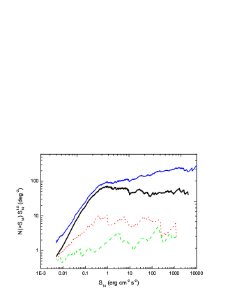
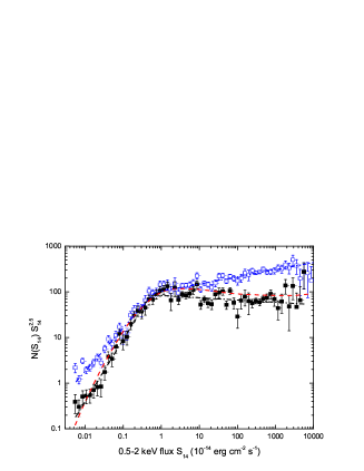
Figure 1: (a) Cumulative number counts N($>$S) for the total sample (upper blue thin line), the AGN–1 subsample (lower black thick line), the AGN–2 subsample (red dotted line) and the galaxy subsample (green dashed line). (b) Differential number counts of the total sample of X–ray sources (open squares) and the AGN–1 subsample (filled squares). The dot-dashed lines refer to broken powerlaw fits to the differential source counts (see text). The dashed red line shows the prediction for type–1 AGN (from has05 ).

3 Number Counts and Resolved Background Fraction

Based on deep surveys with Chandra and XMM-Newton, the X–ray log(N)–log(S) relation has now been determined down to fluxes of $2.4\times 10^{-17}$ erg cm^-2 s^-1, $2.1\times 10^{-16}$ erg cm^-2 s^-1, and $1.2\times 10^{-15}$ erg cm^-2 s^-1 in the 0.5–2, 2-10 and 5-10 keV band, respectively bra01b ; has01 ; ros02 ; mor03 ; bau04 . Figure 1a shows the normalized cumulative source counts $N(>S_{\rm X14})S_{\rm X14}^{1.5}$. The total differential source counts, normalized to a Euclidean behaviour (dN/d$S_{\rm X14}\times S_{\rm X14}^{2.5}$) is shown with open symbols in Figure 1b. Euclidean source counts would correspond to horizontal lines in these graphs. For the total source counts, the well-known broken powerlaw behaviour is confirmed with high precision. A broken power law fitted to the differential source counts yields power law indices of $\alpha_{b}=2.34\pm 0.01$ and $\alpha_{f}=1.55\pm 0.04$ for the bright and faint end, respectively, a break flux of $S_{\rm X14}=0.65\pm 0.10$ and a normalisation of dN/d$S_{\rm X14}=103.5\pm 5.3$ deg^-2 at $S_{\rm X14}=1.0$ with a reduced $\chi^{2}$=1.51. We see that the total source counts at bright fluxes, as determined by the ROSAT All-Sky Survey data, are significantly flatter than Euclidean, consistent with the discussion in has93 . Moretti et al. mor03 , on the other hand, have derived a significantly steeper bright flux slope ($\alpha_{b}\approx 2.8$) from ROSAT HRI pointed observations. This discrepancy can probably be attributed to the selection bias against bright sources, when using pointed observations where the target area has to be excised.

The ROSAT HRI Ultradeep Survey had already resolved 70-80% of the extragalactic 0.5–2 keV XRB into discrete sources, the major uncertainty being in the absolute flux level of the XRB. The deep Chandra and XMM-Newton surveys have now increased the resolved fraction to 85-100% mor03 ; wor04 . Above 2 keV the situation is complicated on one hand by the fact, that the HEAO-1 background spectrum mar80 , used as a reference over many years, has a $\sim 30\%$ lower normalization than several earlier and later background measurements (see e.g. mor03 ). Recent determinations of the background spectrum with XMM-Newton mol04 and RXTE rev03 strengthen the consensus for a 30% higher normalization, indicating that the resolved fractions above 2 keV have to be scaled down correspondingly. On the other hand, the 2-10 keV band has a large sensitivity gradient across the band. A more detailed investigation, dividing the recent 770 ksec XMM-Newton observation of the Lockman Hole into finer energy bins, comes to the conclusion, that the resolved fraction decreases substantially with energy, from over 90% below 2 keV to less than 50% above 5 keV wor04 .

Type–1 AGN are the most abundant population of soft X–ray sources. For the determination of the AGN–1 number counts we include those unidentified sources, which have hardness ratios consistent with AGN–1 (a contribution of $\sim 6\%$, see Table 1). Figure 1 shows, that the break in the total source counts at intermediate fluxes is produced by type–1 AGN, which are the dominant population there. Both at bright fluxes and at the faintest fluxes, type–1 AGN contribute about 30% of the X–ray source population. At bright fluxes, they have to share with clusters, stars and BL-Lac objects, at faint fluxes they compete with type–2 AGN and normal galaxies (see Fig. 1a and bau04 ). A broken power law fitted to the differential AGN–1 source counts yields power law indices of $\alpha_{b}=2.55\pm 0.02$ and $\alpha_{f}=1.15\pm 0.05$ for the bright and faint end, respectively, a break flux of $S_{\rm X14}=0.53\pm 0.05$, consistent with that of the total source counts within errors, and a normalisation of of dN/d$S_{\rm X14}=83.2\pm 5.5$ deg^-2 at $S_{\rm X14}=1.0$ with a reduced $\chi^{2}$=1.26. The AGN–1 differential source counts, normalized to a Euclidean behaviour (dN/d$S_{\rm X14}\times S_{\rm X14}^{2.5}$) is shown with filled symbols in Figure 1.

4 The Soft X–ray Luminosity Function and Space Density Evolution

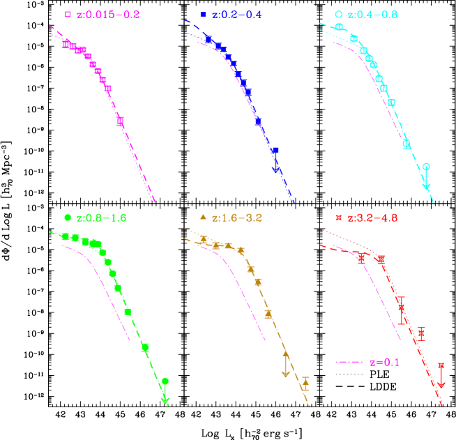
Figure 2: The soft X–ray luminosity function of the type–1 AGN sample in different redshift shells for the nominal case as labelled. The error bars correspond to 68% Poisson errors of the number of AGNs in the bin. The best–fit two power-law model for the $0.015<z<0.2$ shell are overplotted in the higher redshift panels for reference. The dotted and dashed lines give the best–fit PLE and LDDE models (from has05 ).

Hasinger, Miyaji and Schmidt has05 have employed two different methods to derive the AGN–1 X–ray luminosity function and its evolution. The first method uses a variant of the $1\over V_{a}$ method, which was developed in paper1 . The binned luminosity function in a given redshift bin $z_{i}$ is derived by dividing the observed number $N_{obs}(L_{x},z_{i})$ by the volume appropriate to the redshift range and the survey X–ray flux limits and solid angles. To evaluate the bias in this value caused by a gradient of the luminosity function across the bin, each of the luminosity functions is fitted by an analytical function. This function is then used to predict $N_{mdl}(L_{x},z_{i})$. Correcting the luminosity function by the ratio $N_{obs}/N_{mdl}$ takes care of the bias to first order.

The second method uses unbinned data. Individual $V_{\rm max}$ of the RBS sources are used to evaluate the zero-redshift luminosity function. This is free of the bias described above: using this luminosity function to derive the number of expected RBS sources matches the observed numbers precisely. In the subsequent derivation of the evolution, i.e., the space density as a function of redshift, binning in luminosity and redshift is introduced to allow evaluation of the results. Bias at this stage is avoided by iterating the parameters of an analytical representation of the space density function. Together with the zero-redshift luminsity function this is used to predict $N_{mod}(L_{x},z_{i})$ for the surveys. The observed densities in the bins are derived by multiplying the space density value by the ratio $N_{obs}(L_{x},z_{i})/N_{mod}(L_{x},z_{i})$. At this stage, none of the densities are derived by dividing a number by a volume.

The other difference between the two methods is in the treatment of missing redshifts for optically faint objects. In the binned method, all AGN without redshift with $R>24.0$ were assigned the central redshift of each redshift bin to derive an upper boundary to the luminosity function. In the unbinned method, the optical magnitudes of the RBS sources were used to derive the optical redshift limit corresponding to $R=24.0$. The $V_{\rm max}$ values for surveys (such as CDF–N) spectroscopically incomplete beyond $R=24.0$ were based on the smaller of the X–ray and optical redshift limits.

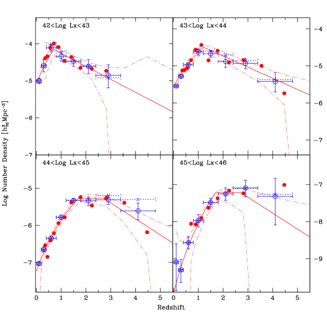
Figure 3: Comparison between the space densities derived with two different methods. The blue datapoints with error bars refer to the binned treatment using the N_obs/N_mdl method, the dashed horizontal lines corresponding to the maximum contribution of unidentified sources. The thin and thick red lines and dots refer to the unbinned method (from has05 ).

Figure 2 shows the luminosity function derived this way in different redshift shells. A change of shape of the luminosity function with redshift is clearly seen and can thus rule out simple density or luminosity evolution models. In a second step, instead of binning into redshift shells, the sample has been cut into different luminosity classes and the evolution of the space density with redshift was computed. Figure 3 shows a direct comparison between the binned and unbinned determinations of the space density, which agree very well within statistical errors.

The fundamental result is, that the space density of lower–luminosity AGN–1 peaks at significantly lower redshift than that of the higher–luminosity (QSO–type) AGN. Also, the amount of evolution from redshift zero to the peak is much less for lower–luminosity AGN. The result is consistent with previous determinations based on less sensitive and/or complete data, but for the first time our analysis shows a high-redshift decline for all luminosities $L_{X}<10^{45}$ erg s^-1 (at higher luminosities the statistics is still inconclusive). Albeit the different approaches and the still existing uncertainties, it is very reassuring that the general properties and absolute values of the space density are very similar in the two different derivations in.

A luminosity-dependent density evolution (LDDE) model has been fit to the data. Even though the sample is limited to soft X–ray-selected type–1 AGN, the parameter values of the overall LDDE model are surprisingly close to those obtained by Ueda et al. 2003 for the intrinsic (de-absorbed) luminosity function of hard X–ray selected obscured and unobscured AGN, except for the normalization, where Ueda et al. reported a value about five times higher.

These new results paint a dramatically different evolutionary picture for low–luminosity AGN compared to the high–luminosity QSOs. While the rare, high–luminosity objects can form and feed very efficiently rather early in the Universe, with their space density declining more than two orders of magnitude at redshifts below z=2, the bulk of the AGN has to wait much longer to grow with a decline of space density by less than a factor of 10 below a redshift of one. The late evolution of the low–luminosity Seyfert population is very similar to that which is required to fit the Mid–infrared source counts and background fra02 and also the bulk of the star formation in the Universe mad98 , while the rapid evolution of powerful QSOs traces more the merging history of spheroid formation fra99 .

This kind of anti–hierarchical Black Hole growth scenario is not predicted in most of the semi–analytic models based on Cold Dark Matter structure formation models (e.g. kau00 ; wyi03 ). This could indicate two modes of accretion and black hole growth with radically different accretion efficiency (see e.g. dus02 ). A self–consistent model of the black hole growth which can simultaneously explain the anti–hierarchical X–ray space density evolution and the local black hole mass function derived from the $M_{BH}-\sigma$ relation assuming two radically different modes of accretion has recently been presented in mer04 .

5 Optical versus X–ray selection of AGN–1

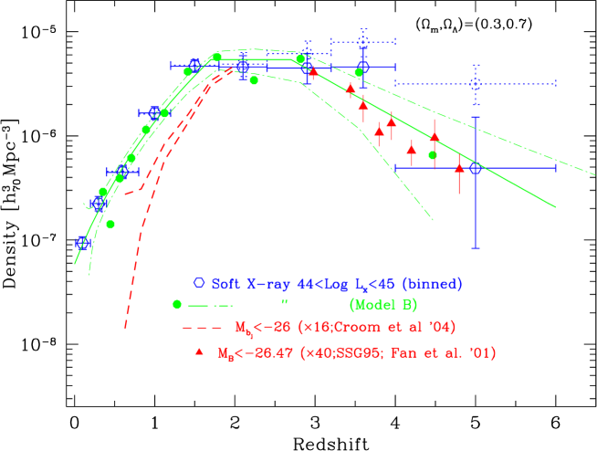
Figure 4: Comparison of the space density of luminous QSOs between optically selected and soft X–ray selected samples (from has05 ). The X–ray number densities are plotted for the luminosity class ${\rm log\,}L_{\rm x}=44-45$, both for the binned and unbinned analysis with the same symbols as in Fig. 3. The dashed lines represent the one sigma range for $M_{b_{r,j}}<-26.0$ from cro04 , multiplied by a factor of 16 to match the X–ray space density at z=2. The triangles at $z>2.7$ with 1$\sigma$ errors are from ssg95 (SSG95) and fan01 after a cosmology conversion (see text) and a scaling by a factor of 40 to match with the soft X–ray density at $z\sim 2.7$. As discussed in this paper, both the rise and the decline of the space density, behavior changes with $L_{x}$ and therefore that the comparison can only be illustrative.

The space density of soft X–ray selected QSOs from the Hasinger et al. sample is compared to the one of optically-selected QSOs at the most luminous end in Fig. 4. The $z<2$ number density curve for optically selected QSOs ($M_{b_{\rm J}}<-26.0$) is from the combination of the 2dF and 6dF QSO redshift surveys cro04 . The $z>2.7$ number densities from ssg95 and fan01 have been originally given for $H_{0}$=50 km s^-1 Mpc${}^{-1},\Omega_{m}=1,\Omega_{\Lambda}=0$. Their data points have been converted to $H_{0}$=70 km s^-1 Mpc${}^{-1},\Omega_{m}=0.3,\Omega_{\Lambda}=0.7$ and the $M_{\rm B}$ threshold has been re-calculated with an assumed spectral index of $\alpha_{o}=-0.79$ ($f_{\nu}\propto\nu^{\alpha_{o}}$), following e.g. vig03 . The plotted curve from ssg95 ; fan01 is for $M_{B}<-26.47$ under these assumptions. A small correction of densities due to the cosmology conversion causing redshift-dependent luminosity thresholds has also been made, assuming $d\Phi/dlogL_{B}\propto L_{B}^{-1.6}$ fan01 . The space density for the soft X–ray QSOs for the luminosity class $44<logL_{x}<45$ has been plotted both for the binned and unbinned determination. The Croom et al. cro04 space density had to be scaled up by a factor of 16 in order to match the X–ray density at $z\sim 2$. The Schmidt, Schneider & Gunn / Fan et al. data points have been scaled by a factor of 40 to match the soft X–ray data at $z=2.7$ in the plot. There is relatively little difference in the density functions between the X–ray and optical QSO samples, although we have to keep in mind, that both the rise and the decline of the space density is varying with X–ray luminosity, so that this comparison can only be illustrative until larger samples of high–redshift X–ray selected QSOs will be available.

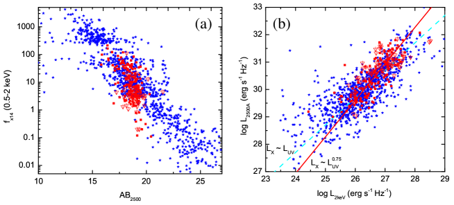
Figure 5: (a): comparison of X–ray fluxes and AB₂₅₀₀ UV magnitudes for the sample of $\sim 1000$ X–ray selected type-1 AGN from has05 (blue points) with the ROSAT-observed optically selected SDSS QSOs vig03 . Filled red squares give the standard SDSS QSO, while open red squares give the specifically selected high-redshift SDSS sample (see vig03 ). (b): Monochromatic 2 keV X–ray versus 2500 $\AA$  UV luminosity for the same samples. The blue (dark) solid line shows a linear relation between the two luminosities, while the yellow (light) solid line gives the non-linear relation $L_{X}\sim L_{UV}^{0.75}$ from the literature vig03 .

As a next step we directly study the X–ray and optical fluxes and luminosities of our sample objects and compare this with the optically selected QSO sample of Vignali et al. vig03 based on SDSS-selected AGN serendipitously observed in ROSAT PSPC pointings. Because of the inhomogeneous nature and different systematics of the different surveys entering our sample, the optical/UV magnitudes of our objects have unfortunately much larger random and systematic errors and are based on fewer colours than the excellent SDSS photometry. In our preliminary analysis we therefore calculated the AB₂₅₀₀ magnitudes simply extrapolating or interpolating the observed magnitudes in the optical filters closest to the redshifted 2500 $\AA$ band, assuming an optical continuum with a power law index of -0.7, i.e. not utilizing the more complicated QSO spectral templates including emission lines which have been used in vig03 . A spectroscopic correction for the host galaxy contamination, as done for the SDSS sample, was also not possible for our sample, however, for a flux and redshift-selected sample of 94 RBS Seyferts salvato we have morphological determinations of the nuclear versus host magnitudes (see below). In all other aspects of the analysis we follow the Vignali et al. treatment. Figure 5a shows 0.5–2 keV X–ray fluxes versus AB₂₅₀₀ magnitudes for our sample objects (blue stars) in comparison with the Vignali et al. SDSS sample (X–ray detections are shown as filled red squares, upper limits as down–pointing triangles). It is obvious, that our multi-cone survey sample covers a much wider range in X–ray and optical fluxes than the magnitude-limited SDSS sample. Unlike the SDSS sample, our sample shows a very clear correlation between X–ray and optical fluxes, but also a wider scatter in this correlation.

Figure 5b shows the monochromatic X–ray versus UV luminosity for the same data. Now the X–ray and optically selected samples cover a similar parameter range at the high luminosity end, but the X–ray selected data reach significantly lower X–ray and UV luminosities than the optically selected sample. Again, there is a larger scatter in the X–ray selected sample. The figure also shows two analytic relations between X–ray and UV luminosity: a linear relation L${}_{X}\propto$L_UV and the non–linear behaviour L${}_{X}\propto$L${}_{UV}^{0.75}$ found in the literature (e.g. vig03 ). While the Vignali et al. optically selected sample clearly prefers the non-linear dependence (see also bra04 ), this is not true for the X-ray selected sample, which is consistent with a linear relation, apart from the behaviour at low luminosities, where significant contamination from the host galaxy is expected.

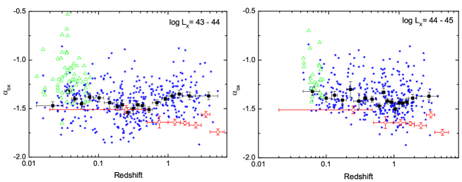
Figure 6: X–ray to optical spectral index $\alpha_{ox}$ as a function of redshift for different luminosity classes for the Hasinger et al. sample of $\sim 1000$ soft X–ray selected type-1 AGN. Blue (dark) stars give the values derived using the total integrated optical light, while the green triangles give the values using only the nuclear component from 93 RBS AGN, derived by Salvato salvato from detailed imaging decomposition. The solid black squares with error bars give the median and variance of the X-ray selected sample. Open red squares with error bars show the average $\alpha_{ox}$ values for the Vignali et al. optically selected QSOs.

To check on any evolution of the optical to X–ray spectral index with redshift we calculated $\alpha_{ox}$ values, following vig03 for all our sample objects. In order to see possible luminosity–dependent evolution effectssimilar to those observed in the space density evolution, we divided our sample into the same luminosity classes as in Section 4. Figure 6 shows the $\alpha_{ox}$ values determined for objects in the luminosity class 43–44 and 44–45, respectively, as a function of redshift. Apart from a few wiggles, which are likely due to the omission of the emission lines in the optical AGN continuum, there is no significant evolution with redshift. The optically selected sample, on the other hand, shows a significant trend with redshift and average values inconsistent with the X-ray selected sample for most of the redshift range. The diagram also shows, that this discrepancy is likely not caused by the missing host galaxy contamination correction in our analysis. From the relatively small number of nearby (z$<$0.1) of RBS sources, where a morphological fitting procedure has been used to subtract the host emission from the total magnitude salvato we can estimate the host dilution effect, which is clearly larger at lower X–ray luminosities and makes the discrepancy even larger. The immediate conclusion is, that the average optical to X-ray sample properties are dependent on systematic sample selection effects.

6 X–ray Constraints on the Growth of SMBH

The AGN luminosity function can be used to determine the masses of remnant black holes in galactic centers, using Sołtan’s continuity equation argument sol82 and assuming a mass-to-energy conversion efficiency $\epsilon$. For a non-rotating Schwarzschild BH, $\epsilon$ is expected to be 0.054, while for a maximally rotating Kerr BH, $\epsilon$ can be as high as 0.37 tho74 . The AGN demography predicted, that most normal galaxies contain supermassive black holes (BH) in their centers, which is now widely accepted (e.g. kor01 and references therein). Recent determinations of the accreted mass from the optical QSO luminosity function are around $2\epsilon_{0.1}^{-1}\cdot 10^{5}M_{\odot}Mpc^{-3}$ cho92 ; yut02 . Estimates from the X–ray background spectrum, including obscured accretion power obtain even larger values: 6-9 fab99 or 8-17 elv02 in the above units, and values derived from the infrared band hae01 or multiwavelength observations bar01b are similarly high (8-9). Probably the most reliable recent determination comes from an integration of the X–ray luminosity function. Using the Ueda et al. ued03 hard X–ray luminosity function including a correction for Compton–thick AGN normalized to the X–ray background, as well as an updated bolometric correction ignoring the IR dust emission, Marconi et al mar04 derived $\rho_{accr}\sim 3.5\epsilon_{0.1}^{-1}\cdot 10^{5}M_{\odot}Mpc^{-3}$.

The BH masses measured in local galaxies are tightly correlated to the galactic velocity dispersion fer00 ; geb00 , and less tightly to the mass and luminosity of the host galaxy bulge (however, see mar03 ). Using these correlations and galaxy luminosity (or velocity) functions, the total remnant black hole mass density in galactic bulges can be estimated. Scaled to the same assumption for the Hubble constant (H₀=70 km s^-1 Mpc^-1), recent papers arrive at different values, mainly depending on assumptions about the intrinsic scatter in the BH–galaxy correlations: $\rho_{BH}$ = ($2.4\pm 0.8$), ($2.9\pm 0.5$) and $(4.6^{+1.9}_{-1.4}h_{70}^{2}\cdot 10^{5}M_{\odot}Mpc^{-3}$, respectively all02 ; yut02 ; mar04 . The local dark remnant mass function is fully consistent with the above accreted mass function, if black holes accrete with an average energy conversion efficiency of $\epsilon=0.1$ mar04 , which is the classically assumed value and lies between the Schwarzschild and the extreme Kerr solution. However, taking also into account the widespread evidence for a significant kinetic AGN luminosity in the form of jets and winds, it is predicted, that the average supermassive black hole should be rapidly spinning fast (see also elv02 ; yut02 ). Recently, using XMM-Newton, a strong relativistic Fe K$\alpha$ line has been discovered in the average rest–frame spectra of AGN–1 and AGN–2 stre05 , which can be best fit by a rotating Kerr solution consistent with this conjecture.

Acknowledgements I thank my colleagues in the Chandra Deep Field South and XMM–Newton Lockman Hole projects, as well as Maarten Schmidt, Takamitsu Miyaji and Niel Brandt for the excellent cooperation on studies of the X–ray background.

References

- (1) Alexander D.M., Aussel, H., Bauer F.E., et al., ApJ, 568, L85 (2002)
- (2) Alexander D.M., Bauer F.E., Brandt W.N., et al., AJ, 126, 539 (2003)
- (3) Aller, M. C., Richstone, D., AJ 124, 3035 (2002)
- (4) Appenzeller, I., Thiering, I., Zickgraf, F.-J., et al., A&A (Suppl.) 364, 443 (1998)
- (5) Barger A. J., Cowie L. L., Mushotzky R. F., Richards, E. A., AJ 121, 662 (2001a)
- (6) Barger A J, Cowie L L, Bautz M W, Brandt W N, Garmire G P, et al., AJ, 122, 2177 (2001b)
- (7) Barger A.J., Cowie L.L., Capak P., et al., AJ, 126, 632 (2003)
- (8) Bauer F.E., Alexander D.M., Brandt W.N., et al., AJ in press, astro-ph/0408001 (2004)
- (9) Bower R. G., Hasinger, G., Castander, F. J. et al., MNRAS 281, 59 (1996)
- (10) Brandt W. N., Alexander, D. M., Hornschemeier, A. E., Garmire, G. P., Schneider, D. P., et al., AJ 122, 2810 (2001)
- (11) Brandt, W.N., Vignali C., Lehmer B.D., et al., this volume (2005)
- (12) Brandt, W. N., Hasinger, G., ARAA in press (2005)
- (13) Chokshi, A., Turner, E. L., MNRAS 259, 421 (1992)
- (14) Croom, S. M., Smith, R. J., Boyle, B. J., Shanks, T., Miller, L., et al., MNRAS 349, 1397 (2004)
- (15) De Luca, A., Molendi, S., A&A 419, 837
- (16) Duschl, W.J., Strittmatter, P.A., in Active Galactic Nuclei: from Central Engine to Host Galaxy Abstract Book, meeting held in Meudon, France, July 23-27, 2002, Eds.: S. Collin, F. Combes and I. Shlosman. To be published in ASP Conference Series, p. 76 (2002)
- (17) Elvis, M., Risaliti, G., & Zamorani, G., ApJ 565, L75 (2002)
- (18) Fabian, A. C., Iwasawa, K., MNRAS 303, 34 (1999)
- (19) Fadda, D., Flores, H., Hasinger, G., et al., A&A 383, 838 (2002)
- (20) Fan, X., Strauss, M. A., Schneider, D. P., Gunn, J. E., Lupton, R. H., et al., AJ 121, 54 (2001)
- (21) Ferrarese, L., Merritt, D., ApJ 539, L9 (2000)
- (22) Fiore F., Brusa M., Cocchia F., et al., A&A 409, 79 (2003)
- (23) Franceschini, A., Hasinger, G., Miyaji, T., Malquori, D., MNRAS 310, L15 (1999)
- (24) Franceschini A., Braito V. & Fadda D., MNRAS, 335, L51 (2002)
- (25) Gebhardt, K., Bender, R., Bower, G., Dressler, A., Faber S. M., et al., ApJ 539, L13 (2000)
- (26) Giacconi R., Rosati P., Tozzi P., et al., ApJ, 551, 624 (2001)
- (27) Giacconi, R., Zirm, A., Wang, J.X., et al., ApJS, 139, 369 (2002)
- (28) Gilli, R., Cimatti, A., Daddi, E., et al., ApJ 592, 721 (2003)
- (29) Gioia, I., Henry, J.P., Mullis, C.R., et al., ApJS 149, 29 (2003)
- (30) Haehnelt, M. G., Kauffmann, G., in Black Holes in Binaries and Galactic Nuclei, ed. L. Kaper, E. P. J. van den Heuvel, & P. A. Woudt, p.364 (Berlin: Springer) (2001)
- (31) Hasinger G., Burg R., Giacconi R., et al., A&A 275, 1 (1993)
- (32) Hasinger G., Burg R., Giacconi R., et al., A&A 329, 482 (1998)
- (33) Hasinger G., Altieri B., Arnaud M., et al., A&A 365, 45 (2001)
- (34) Hasinger, G., Miyaji, T., Schmidt, M., A&A submitted (2005)
- (35) Hornschemeier A.E., Brandt W.N., Garmire G.P., et al., ApJ 541, 49 (2000)
- (36) Hornschemeier A.E., Bauer F.E., Alexander D.M., et al., AJ 126, 575 (2003)
- (37) Kauffmann, G. & Haehnelt, M., MNRAS 311, 576 (2000)
- (38) Kormendy, J., Gebhardt, K., AIP conference proceedings 586, 363 (2001)
- (39) Lehmann I., Hasinger G., Schmidt M., et al., A&A 354, 35 (2000)
- (40) Lehmann I., Hasinger G., Schmidt M., et al., A&A 371, 833 (2001)
- (41) Madau, P., Pozzetti, L., Dickinson, M., ApJ 498, 106 (1998)
- (42) Mainieri V., Bergeron J., Rosati P., et al., A&A 393, 425 (2002)
- (43) Mainieri V., Rosati P., Tozzi, P., et al., A&A submitted (2004)
- (44) Marconi, A., Hunt, L. K. ApJ 589, L21 (2003)
- (45) Marconi, A., Risaliti, G., Gilli, R., Hunt, L. K., Maiolino, R., Salvati, M., MNRAS 351, 169 (2004)
- (46) Marshall, F. E., Boldt, E. A., Holt, S. S., et al., ApJ 235, 4 (1980)
- (47) Mason K. O., Carrera, F. J., Hasinger, G., et al., MNRAS 311, 456 (2000)
- (48) McHardy I.M., Jones, L. R., Merrifield, M. R., et al., MNRAS, 295, 641 (1998)
- (49) Merloni, A., MNRAS 353, 1035 (2004)
- (50) Miyaji, T., Hasinger G., Schmidt M., A&A 353, 25 (2000)
- (51) Miyaji, T., Hasinger, G., Schmidt, M., A&A 369, 49 (2001)
- (52) Moran, E. C., Filippenko, A. V. & Chornock, R., ApJ 579, L71 (2002)
- (53) Moretti, A., Campana, S., Lazzati, D., et al., ApJ 588, 696 (2003)
- (54) Mullis, C. R., Henry, J. P., Gioia, I. M., et al., ApJ submitted (astro-ph/0408304) (2004)
- (55) Mushotzky, R. F., Cowie, L. L., Barger, A. J., Arnaud, K. A., Nature 404, 459 (2000)
- (56) Norman, C., Ptak, A., Hornschemeier, A., et al., ApJ 607, 721 (2004)
- (57) Revnivtsev, M., Gilfanov, M., Sunyaev, R., et al., A&A 411, 329 (2003)
- (58) Rosati P., Tozzi P., Giacconi R., et al., ApJ 566, 667 (2002)
- (59) Salvato, M., Dissertation, Potsdam University (2002)
- (60) Schmidt, M., Schneider, D. P., Gunn, J. E., AJ 110, 68 (1995)
- (61) Schmidt, M., Hasinger, G., Gunn, J. E., et al., A&A 329, 495 (1998)
- (62) Schwope A., Hasinger, G., Lehmann, I., et al., AN, 321, 1 (2000)
- (63) Sołtan, A., MNRAS 200, 115 (1982)
- (64) Streblyanska, A., Hasinger, G., Finoguenov, A. et al., A&A in press (2005)
- (65) Szokoly G., Bergeron J., Hasinger G., et al., ApJS in press (astro-ph/0312324) (2004)
- (66) Thorne, K. S., ApJ 191, 507 (1974)
- (67) Tozzi, P., Rosati, P., Nonino, M., et al., ApJ 562, 42 (2001)
- (68) Ueda, Y., Akiyama, M., Ohta, K., Miyaji, T., ApJ 598, 886 (2003)
- (69) Vignali C., Brandt W.N., Schneider D.P., AJ 125, 433 (2003)
- (70) Worsley, M., Fabian, A.C., Mateos, S., et al., MNRAS 352, L28 (2004)
- (71) Wyithe, J.S.B., Loeb, A., ApJ 595, 614 (2003)
- (72) Yang, Y., Mushotzky, R. F., Barger, A. J., et al., ApJ 585, L85 (2003)
- (73) Yu, Q., Tremaine, S., MNRAS 335, 965 (2002)
- (74) Zamorani, G., et al. A&A, 346, 731 (1999)
- (75) Zheng W., Mikles, V. J., Mainieri, V., et al., ApJ in press, astro-ph/0406482 (2004)