CMB Anisotropy of the Poincaré Dodecahedron

Abstract

We analyse the anisotropy of the cosmic microwave background (CMB) for the Poincaré dodecahedron which is an example for a multi-connected spherical universe. We compare the temperature correlation function and the angular power spectrum for the Poincaré dodecahedral universe with the first-year WMAP data and find that this multi-connected universe can explain the surprisingly low CMB anisotropy on large scales found by WMAP provided that the total energy density parameter $\Omega_{\hbox{\scriptsize tot}}$ is in the range $1.016\dots 1.020$. The ensemble average over the primordial perturbations is assumed to be the scale-invariant Harrison-Zel’dovich spectrum. The circles-in-the-sky signature is studied and it is found that the signal of the six pairs of matched circles could be missed by current analyses of CMB sky maps.

astro-ph/0412569

1 Introduction

The question of the global geometry of the Universe, i. e. of its spatial curvature, topology and thus its shape, is a very fundamental one. While the problem of the spatial curvature is discussed in all textbooks on cosmology, mainly in connection with the total mass/energy densities in the Universe and the various inflationary scenarios, the possibility of a multi-connected Universe is only rarely mentioned. This is surprising in view of the fact that it was already realized before Einstein’s seminal first paper on cosmology [1] that the three-dimensional space of astronomy might be not only non-Euclidean, but also multi-connected according to a given Clifford-Klein space form (see e. g. [2]). If the Universe is assumed to be simply connected, the cosmological principle implies that it is not only locally, but also globally isotropic and homogeneous. This means that all spatial points are geometrically equivalent. In the case of a multi-connected Universe, however, the cosmological principle holds in general only on the universal covering space of constant curvature, i. e. on ${\cal E}^{3}$, ${\cal S}^{3}$ and ${\cal H}^{3}$ for a flat, positively and negatively curved Universe, respectively. While the Einstein gravitational field equations still hold in a multi-connected Universe, the global structure of the Universe at large scales will be more complicated.

The discovery of the temperature fluctuations $\delta T$ of the cosmic microwave background radiation (CMB) by COBE in 1992 [3] and the detailed measurements by WMAP [4] and by other groups have led to a renewed interest in the question of the global geometry of the Universe (see [5, 6] for reviews).

The most promising signatures to detect a possible multi-connected spatial structure of the Universe are the strange suppression of the CMB quadrupole and octopole, and of the temperature correlation function first observed by COBE [7] and nicely confirmed by WMAP [4], and the so-called circles-in-the-sky-signature proposed in [8].

Until about 1999, all observational data were consistent with the fact that the total energy density $\varepsilon_{\hbox{\scriptsize tot}}$ (at the present epoch) amounted only to ca. 30% of the critical energy density $\varepsilon_{\hbox{\scriptsize crit}}=\frac{3H_{0}c^{2}}{8\pi G}$, i. e. $\Omega_{\hbox{\scriptsize tot}}:=\varepsilon_{\hbox{\scriptsize tot}}/\varepsilon_{\hbox{\scriptsize crit}}\simeq 0.3<1$, and thus strongly indicated that the geometry of the Universe is hyperbolic. Consequently, several groups performed detailed studies of compact and non-compact models of the Universe possessing hyperbolic geometry. Although later observations on the magnitude redshift relation of the supernovae of type Ia [9, 10] provided evidence for a large dark energy component, and the determination of the first acoustic peak in the CMB anisotropy by TOCO [11, 12], BOOMERanG [13] and MAXIMA-1 [14, 15] indicated a nearly flat Universe, i. e. $\Omega_{\hbox{\scriptsize tot}}\simeq 1$, the available data are still compatible with the spatial geometry of the Universe being hyperbolic. (For a discussion of hyperbolic universes, see [16, 17, 18, 19, 20, 21, 22, 23, 24, 25, 26, 27].)

The concordance model of cosmology assumes an exactly (spatially) flat Universe with the topology of ${\cal E}^{3}$ and, furthermore, that the dark energy is given by a positive cosmological constant $\Lambda$, i. e. $\Omega_{\Lambda}:=\frac{\Lambda c^{2}}{3H_{0}^{2}}=1-\Omega_{\hbox{\scriptsize mat}}-\Omega_{\hbox{\scriptsize rad}}$ with $\Omega_{\hbox{\scriptsize mat}}=\Omega_{\hbox{\scriptsize bar}}+\Omega_{\hbox{\scriptsize cdm}}$, where the various parameters denote the present values of the baryonic (bar), cold dark matter (cdm), matter (mat) and radiation (rad) energy densities in units of $\varepsilon_{\hbox{\scriptsize crit}}$ ($\Lambda$CDM model). In the following, we shall refer to three variants of the concordance model presented by the WMAP team on the Legacy Archive for Microwave Background Data Analysis (LAMBDA) Web site http://lambda.gsfc.nasa.gov, see also [28]. These models give a good overall fit to the CMB anisotropy on small and medium scales, but there remains a strange discrepancy at large scales as first observed by COBE [7] and later substantiated by WMAP [4].

Let us expand the temperature fluctuations $\delta T(\hat{n})$ of the microwave sky, where the dipole contribution has been subtracted, into real spherical harmonics $\tilde{Y}_{lm}(\hat{n})$ on ${\cal S}^{2}$,

$$\delta T(\hat{n})\;:=\;\sum_{l=2}^{\infty}\sum_{m=-l}^{l}\,a_{lm}\,\tilde{Y}_{lm}(\hat{n})\hskip 10.0pt,$$ (1)

where $\hat{n}$ denotes the unit vector in the direction from which the photons arrive. (Note that the monopole and dipole terms, $l=0,1$, are not included in the sum (1).) From the real expansion coefficients $a_{lm}$ one forms the multipole moments

$$C_{l}\;:=\;\frac{1}{2l+1}\,\Big{<}\sum_{m=-l}^{l}\,\big{(}a_{lm}\big{)}^{2}\,\Big{>}$$ (2)

and the angular power spectrum

$$\delta T_{l}^{2}\;:=\;\frac{l(l+1)}{2\pi}\,C_{l}\hskip 10.0pt.$$ (3)

The average $\left<\dots\right>$ in (2) denotes an ensemble average over the primordial perturbations to be discussed in section 4, respectively an ensemble average over the universal observers. The temperature two-point correlation function $C(\vartheta)$ is defined as $C(\vartheta):=\left<\delta T(\hat{n})\delta T(\hat{n}^{\prime})\right>$ with $\hat{n}\cdot\hat{n}^{\prime}=\cos\vartheta$, which can be computed from the multipole moments (2) under the assumption of statistical isotropy as

$$C(\vartheta)\;\simeq\;\frac{1}{4\pi}\,\sum_{l=2}^{\infty}\,(2l+1)\,C_{l}\,P_{l}(\cos\vartheta)\hskip 10.0pt.$$ (4)

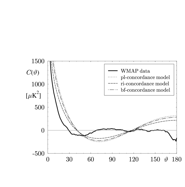
Figure 1: $C(\vartheta)$ from first year WMAP data (solid curve) in comparison to the three concordance models provided by the WMAP team at http://lambda.gsfc.nasa.gov: model pl assumes a power law fit to the WMAP, CBI and ACBAR data, model ri assumes a running index fit to the WMAP, CBI and ACBAR data, and finally, model bf assumes a running index fit to the WMAP, CBI and ACBAR data and additionally takes the large scale data from 2dF and Ly-alpha into account.

In figure 1 we show $C(\vartheta)$ as solid curve as measured by WMAP [4]. The important conclusion to be drawn from figure 1 is that the temperature correlation function displays very weak correlations at wide angles, $60^{\circ}\lesssim\vartheta\lesssim 160^{\circ}$. The data are compared with three different versions of the concordance model obtained by the WMAP team as best fits of their data combined with various other data. The model pl (dotted curve) assumes a power law fit, i. e. with no running index, to the WMAP [4], CBI [29, 30] and ACBAR [31] data, the model ri (dashed curve) assumes a running index fit to the WMAP, CBI and ACBAR data, and finally, the model bf (dashed-dotted curve) assumes again a running index fit to the WMAP, CBI and ACBAR data and additionally takes the large scale structure data from 2dF [32] and Lyman-$\alpha$ [33] into account. It is seen from figure 1 that the difference between the three concordance models is not considerable. One makes, however, the important observation that the three concordance models using the best-fit values for the cosmological parameters as obtained by WMAP do not reproduce the experimentally observed suppression of power at wide angles, leaving us with “the mystery of the missing fluctuations” [34]. In the case of the largest angles, $160^{\circ}\lesssim\vartheta\leq 180^{\circ}$, where the WMAP curve in figure 1 shows even negative temperature correlations, one might argue that the measurements in the nearly back-to-back configuration are very subtle due to the need to apply a Galactic cut to the data and, furthermore, due to geometrical reasons, since the expectation values of $C(\vartheta)$ are computed from a much smaller number of pixels, and thus the discrepancy at these angles should not be overemphasized. There is, however, also a discrepancy between the three concordance models and the WMAP data at small angles, $\vartheta\lesssim 40^{\circ}$, which is clearly visible in figure 1.

Depending on certain priors, the WMAP team reported [28] for the total energy density $\Omega_{\hbox{\scriptsize tot}}=1.02\pm 0.02$ together with $\Omega_{\hbox{\scriptsize bar}}=0.044\pm 0.004$, $\Omega_{\hbox{\scriptsize mat}}=0.27\pm 0.04$, and $h=0.71_{-0.03}^{+0.04}$ for the present day reduced Hubble constant (the errors give the $1\sigma$-deviation uncertainties). Taken at their face value, these parameters hint to a positively curved Universe. Recently Luminet et al. [35] studied the Poincaré dodecahedral space (for details, see section 2) which is one of the well-known space forms with constant positive curvature (see also [36, 37, 34]). The authors of ref. [35] computed the CMB multipoles for $l=2,3$ and 4, fitted the overall normalization factor to match the WMAP data at $l=4$, and then examined the prediction for $l=2$ and $l=3$ as a function of $\Omega_{\hbox{\scriptsize tot}}$. For $\Omega_{\hbox{\scriptsize tot}}=1.013$ they found a strong suppression of the power at $l=2$ and weak suppression at $l=3$ in agreement with the WMAP data. Since the eigenfunctions of the Poincaré dodecahedron are not known analytically, they must be computed numerically [38, 39]. In ref. [35], only the first three modes with wave number $\beta=13,21$ and 25 (comprising in total 59 eigenfunctions) have been used, which in turn restricted the discussion to the multipoles $l\leq 4$. There thus remains the question about how this extremely low wave number cut-off affects the prediction of the multipoles, since experience shows that increasing the cut-off usually enhances the integrated Sachs-Wolfe contribution.

In this paper, we present a thorough discussion of the CMB anisotropy for the dodecahedral space topology which is based on the computation of the first 10521 eigenfunctions corresponding to the large wave number cut-off $\beta=155$. Taking within the tight-coupling approximation not only the ordinary, but also the integrated Sachs-Wolfe and also the Doppler effect into account, we are able to predict sufficiently many multipole moments such that a detailed comparison of the dodecahedral model with the WMAP data can be performed. We find that the temperature correlation function for the dodecahedral universe possesses very weak correlations at large scales in nice agreement with the WMAP data for $\Omega_{\hbox{\scriptsize tot}}$ in the range $1.016\dots 1.020$. Besides the suppression of large-scale fluctuations, the dodecahedral model predicts 6 pairs of matching circles in the sky possessing an angular radius of $40^{\circ}\dots 50^{\circ}$ for the slight curvature of space corresponding to the cited range of $\Omega_{\hbox{\scriptsize tot}}$.

We begin in section 2 by describing the spherical space forms and, in particular, the Poincaré dodecahedron, and discuss the general properties of the vibrational modes. In section 3, we outline our numerical method to determine the eigenmodes numerically. In section 4, we calculate the angular power spectrum and the temperature correlation function for the dodecahedral space and compare the predictions with the WMAP data. As a quantitative test, we study the $S$ statistic introduced in [28]. For this statistic, it is found that nice agreement with the WMAP data is obtained for $\Omega_{\hbox{\scriptsize tot}}=1.016\dots 1.020$. In section 5, we study the circles-in-the-sky signature using a quantity $\Sigma$ introduced in [8] (called $S$ in [8]). In the last section, there is a discussion and summary.

2 The spherical space forms and their vibrational modes

The three-dimensional spaces ${\cal M}^{3}$ of constant positive curvature $K=+1$ (spherical spaces) were classified by 1932 [40, 41] and are given by the quotient ${\cal M}^{3}={\cal S}^{3}/\Gamma$ of the 3-sphere ${\cal S}^{3}$ under the action of a discrete fixed-point free subgroup $\Gamma\subset\hbox{SO(4)}$ of the isometries of ${\cal S}^{3}$. All these manifolds are compact and are, apart from their universal covering ${\cal S}^{3}$, multi-connected.

The unit 3-sphere ${\cal S}^{3}$ is defined as the three-dimensional hypersurface of the four-dimensional unit ball in flat four-dimensional space with Cartesian coordinates $(w,x,y,z)\in\mathbb{R}^{4}$, i. e. ${\cal S}^{3}$ is given by the set of points which satisfy the condition $w^{2}+x^{2}+y^{2}+z^{2}\;=\;1$. The spatial distance $|d\vec{x}\,|$ between neighbouring points is given by

$$d\vec{x}\,^{2}\;=\;dw^{2}+dx^{2}+dy^{2}+dz^{2}\hskip 10.0pt,$$ (5)

and the full four-dimensional space-time line element reads

$$ds^{2}\;=\;c^{2}dt^{2}-R^{2}(t)\,d\vec{x}\,^{2}\;=\;a(\eta)^{2}\left[d\eta^{2}-d\vec{x}\,^{2}\right]\hskip 10.0pt.$$ (6)

Here $R(t)=a(\eta)$ denotes the cosmic scale factor as a function of cosmic time $t$ respectively conformal time $\eta$ $(d\eta=c\,dt/R(t))$. The metric (6) has the most general form assuming that the Universe is homogeneous and isotropic (cosmological principle).

The condition $w^{2}+x^{2}+y^{2}+z^{2}\;=\;1$ can be used to eliminate one spatial coordinate, $w$ say, and one is left with the three space variables $(x,y,z)$. In the following, we shall also use the three angular variables $(\chi,\theta,\phi)$ defined by

$$w = \cos\chi\hskip 10.0pt,\hskip 10.0ptx\;=\;\sin\chi\sin\theta\cos\phi\hskip 10.0pt,$$

$$y = \sin\chi\sin\theta\sin\phi\hskip 10.0pt,\hskip 10.0ptz\;=\;\sin\chi\cos\theta\hskip 10.0pt,$$ (7)

with $0\leq\chi\leq\pi$, $0\leq\theta\leq\pi$, $0\leq\phi\leq 2\pi$. It is seen from (7) that $(x,y,z)$ describe for a fixed value of $\chi$ an ${\cal S}^{2}$-sphere with radius $\sin\chi$ and volume $V^{{\cal S}^{2}}(\chi)=\pi(2\chi-\sin 2\chi)$, where $\theta$ and $\phi$ play the familiar rôle of polar and azimuth angle. The ${\cal S}^{2}$-sphere with radius $\sin\chi$ can be considered as a cross section of the unit ${\cal S}^{3}$-sphere. Varying $\chi$ between 0 and $\pi$, one obtains an infinite sequence of cross sections (=2-spheres) of ${\cal S}^{3}$, whose radius grows from 0 to 1 (for $0\leq\chi\leq\frac{\pi}{2}$), and then shrinks again to zero (for $\frac{\pi}{2}\leq\chi\leq\pi$), which provides a useful way to visualize the 3-sphere.

With (5) and (7), the line element on ${\cal S}^{3}$ can be rewritten as

$$d\vec{x}\,^{2}\;=\;d\chi^{2}\,+\,\sin^{2}\chi\,(d\theta^{2}+\sin^{2}\theta\,d\phi^{2})$$ (8)

which has to be inserted into eq. (6).

For a study of the large-scale anisotropies in the CMB produced by scalar perturbations, we need the (regular) eigenmodes of the covariant Laplacian $\Delta$ on ${\cal S}^{3}$, i. e. the solutions of the Helmholtz equation $(\Delta+E^{{\cal S}^{3}})\Psi^{{\cal S}^{3}}=0$ describing the vibrations on ${\cal S}^{3}$. Using the coordinates $(\chi,\theta,\phi)$ and the metric (8) and separating the variables, the normalized solutions read [42, 43, 44, 45, 46, 47] $(\beta\in\mathbb{N};l=0,1,\dots,\beta-1;m=-l,-l+1,\dots,l)$

$$\Psi_{\beta lm}^{{\cal S}^{3}}(\vec{x}\,)\;=\;R_{\beta l}(\chi)\,\tilde{Y}_{lm}(\theta,\phi)\hskip 10.0pt.$$ (9)

Here $\tilde{Y}_{lm}(\theta,\phi)$ are real spherical harmonics on the unit sphere ${\cal S}^{2}$, and the “radial functions” $R_{\beta l}(\chi)$ are given by

$$R_{\beta l}(\chi)\;=\;A_{\beta l}\,(\sin\chi)^{l}\,C_{\beta-l-1}^{l+1}(\cos\chi)\hskip 10.0pt,$$ (10)

where $C_{\mu}^{\nu}(x)$ are the Gegenbauer polynomials (which can also be expressed in terms of the associated Legendre functions $P_{\mu}^{\nu}(x)$). The normalization factor in (10)

$$A_{\beta l}\;=\;2^{l+\frac{1}{2}}\,l!\,\sqrt{\frac{\beta}{\pi}\,\frac{(\beta-l-1)!}{(\beta+l)!}}$$ (11)

follows from the orthonormality relations

$$\int_{{\cal S}^{3}}d\mu(\vec{x}\,)\,{\Psi^{{\cal S}^{3}}_{\beta lm}}(\vec{x}\,)\,\Psi^{{\cal S}^{3}}_{\beta^{\prime}l^{\prime}m^{\prime}}(\vec{x}\,)\;=\;\delta_{\beta\beta^{\prime}}\,\delta_{ll^{\prime}}\,\delta_{mm^{\prime}}\hskip 10.0pt,$$ (12)

$$\int_{0}^{\pi}d\chi\,\sin^{2}\chi\,R_{\beta l}(\chi)\,R_{\beta^{\prime}l}(\chi)\;=\;\delta_{\beta\beta^{\prime}}\hskip 10.0pt.$$ (13)

The volume element on ${\cal S}^{3}$ reads (with the standard expression $d\Omega=\sin\theta d\theta d\phi$ on ${\cal S}^{2}$)

$$d\mu(\vec{x}\,)\;=\;\sin^{2}\chi\,d\chi\,d\Omega\hskip 10.0pt.$$ (14)

Notice that the radial functions $R_{\beta l}(\chi)$ are even or odd (depending on whether $\beta-l-1$ is an even or odd integer) about the equator $\chi=\frac{\pi}{2}$, since they satisfy the periodic boundary condition

$$R_{\beta l}(\pi-\chi)\;=\;(-1)^{\beta-l-1}\,R_{\beta l}(\chi)\hskip 10.0pt.$$ (15)

Since ${\cal S}^{3}$ is compact, the vibrational modes are discrete,

$$E_{\beta}^{{\cal S}^{3}}\;=\;\beta^{2}-1\hskip 10.0pt,$$ (16)

where $\beta\in\mathbb{N}$ plays the rôle of the wave number. The fundamental mode of ${\cal S}^{3}$ has an eigenvalue of $E_{1}^{{\cal S}^{3}}=0$ corresponding to the constant wave function $\Psi^{{\cal S}^{3}}_{100}=1/\sqrt{V^{{\cal S}^{3}}}$, where $V^{{\cal S}^{3}}=\int_{{\cal S}^{3}}d\mu(\vec{x}\,)=2\pi^{2}$ is the volume of the unit sphere ${\cal S}^{3}$. Since the eigenvalues of ${\cal S}^{3}$ do not depend on $l$ and $m$, the modes are degenerate, and the multiplicity of the mode $\beta$ is given by

$$r^{{\cal S}^{3}}(\beta)\;=\;\sum_{l=0}^{\beta-1}(2l+1)\;=\;\beta^{2}\hskip 10.0pt.$$ (17)

If $N^{{\cal S}^{3}}(k)$ denotes the number of the vibrational modes on ${\cal S}^{3}$ with wave number smaller than or equal to $k\in\mathbb{N}$, we obtain

$$N^{{\cal S}^{3}}(k)\;=\;\sum_{\beta=1}^{k}r^{{\cal S}^{3}}(\beta)\;=\;\frac{1}{3}\,k^{3}\,+\,\frac{1}{2}\,k^{2}\,+\,\frac{1}{6}\,k\;=\;\frac{V^{{\cal S}^{3}}}{6\pi^{2}}\,k^{3}\,+\,O(k^{2})$$

in agreement with Weyl’s asymptotic law for $k\to\infty$.

We now turn to the multi-connected spherical spaces ${\cal S}^{3}/\Gamma$, $\Gamma\subset\hbox{SO(4)}$, possessing the volume $V({\cal S}^{3}/\Gamma)=V^{{\cal S}^{3}}/N$, where $N$ denotes the order of the group $\Gamma$. (For reviews, see [40, 41, 48, 49, 50]). To define the discrete fixed-point free subgroups $\Gamma\subset\hbox{SO(4)}$ of the isometries of ${\cal S}^{3}$, it is advantageous to work with Hamilton quaternions $q:=w+x\hbox{\rm i}+y\hbox{\rm j}+z\hbox{\rm i}\hbox{\rm j}$, $(w,x,y,z)\in\mathbb{R}^{4}$, which are spanned by the 4 basis quaternions $\{1,\hbox{\rm i},\hbox{\rm j},\hbox{\rm i}\hbox{\rm j}\}$, with the multiplication defined by $\hbox{\rm i}^{2}=\hbox{\rm j}^{2}=-1$, $\hbox{\rm i}\hbox{\rm j}=-\hbox{\rm j}\hbox{\rm i}$ plus the property that i and j commute with every real number. The multiplication of quaternions is associative, but not commutative. If $q^{\star}:=w-x\hbox{\rm i}-y\hbox{\rm j}-z\hbox{\rm i}\hbox{\rm j}$ denotes the quaternion conjugate to $q$, the norm of $q$ is defined by $|q|^{2}:=qq^{\star}=w^{2}+x^{2}+y^{2}+z^{2}$. Quaternions with norm $1$ are called unit quaternions. For a unit quaternion $q$, there exists an inverse $q^{-1}$ which is simply given by $q^{-1}=q^{\star}$. It is obvious that the unit 3-sphere ${\cal S}^{3}$ can be identified with the multiplicative group of unit quaternions. The distance $d(q_{1},q_{2})$ between any two points $q_{1}$ and $q_{2}$ on ${\cal S}^{3}$ is given by $\cos d(q_{1},q_{2})=w_{1}w_{2}+x_{1}x_{2}+y_{1}y_{2}+z_{1}z_{2}$ and is a point-pair invariant, i. e. $d(\gamma q_{1},\gamma q_{2})=d(q_{1},q_{2})$ $\forall\gamma\in\hbox{SO(4)}$.

The group SO(4) is isomorphic to ${\cal S}^{3}\times{\cal S}^{3}/\{\pm(1,1)\}$, the two factors corresponding to the left and right group actions. In the following, we are only interested in subgroups $\Gamma\in\hbox{SO(4)}$ which lead to homogeneous manifolds ${\cal S}^{3}/\Gamma$. Such groups possess only so-called right-handed Clifford translations. A quaternion $\gamma\in\Gamma$ corresponds to a Clifford translation, if it translates all points $q_{1},q_{2}\in{\cal S}^{3}$ by the same distance $\chi$, i. e. $d(q_{1},\gamma q_{1})=d(q_{2},\gamma q_{2})=\chi$. The right-handed Clifford transformations $\gamma_{k}\in\Gamma$ in ${\cal S}^{3}$ are defined by left-multiplication of an arbitrary unit quaternion $q\in{\cal S}^{3}$ by $\gamma_{k}:=a_{k}+b_{k}\hbox{\rm i}+c_{k}\hbox{\rm j}+d_{k}\hbox{\rm i}\hbox{\rm j}$, i. e.

$$q\;\mapsto\gamma_{k}\,q = \left(a_{k}+b_{k}\hbox{\rm i}+c_{k}\hbox{\rm j}+d_{k}\hbox{\rm i}\hbox{\rm j}\right)\,\cdot\,\left(w+x\hbox{\rm i}+y\hbox{\rm j}+z\hbox{\rm i}\hbox{\rm j}\right)$$

$$= \left(a_{k}w-b_{k}x-c_{k}y-d_{k}z\right)$$

$$\,+ \left(b_{k}w+a_{k}x-d_{k}y+c_{k}z\right)\,\hbox{\rm i}$$

$$\,+ \left(c_{k}w+d_{k}x+a_{k}y-b_{k}z\right)\,\hbox{\rm j}$$

$$\,+ \left(d_{k}w-c_{k}x+b_{k}y+a_{k}z\right)\,\hbox{\rm i}\hbox{\rm j}\hskip 10.0pt.$$

The right-handed Clifford translation (2) acts as a right-handed corkscrew fixed-point free rotation of ${\cal S}^{3}$.

For our numerical computations of the eigenfunctions, it is convenient to represent the action (2) of a group element $\gamma_{k}\in\Gamma$ by the following orthogonal $4\times 4$ matrix $M_{k}$

$$M_{k}\;=\;\left(\begin{tabular}[]{rrrr}$a_{k}$&$-b_{k}$&$-c_{k}$&$-d_{k}$\\ $b_{k}$&$a_{k}$&$-d_{k}$&$c_{k}$\\ $c_{k}$&$d_{k}$&$a_{k}$&$-b_{k}$\\ $d_{k}$&$-c_{k}$&$b_{k}$&$a_{k}$\end{tabular}\right)\hskip 10.0pt,$$ (19)

which acts from the left in an obvious way on the basis quaternions $(1,\hbox{\rm i},\hbox{\rm j},\hbox{\rm i}\hbox{\rm j})$.

The following groups lead to homogeneous manifolds ${\cal S}^{3}/\Gamma$ [40, 41, 48, 49]:

• The cyclic groups $Z_{n}$ of order $n$ $(n\geq 1)$.

• The binary dihedral groups $D_{m}^{\star}$ of order $4m$ $(m\geq 2)$.

• The binary tetrahedral group $T^{\star}$ of order $24$.

• The binary octahedral group $O^{\star}$ of order $48$.

• The binary icosahedral group $I^{\star}$ of order $120$.

Let us consider the binary icosahedral group $I^{\star}$ in more detail consisting of $N=120$ group elements. They are generated by the two right-handed Clifford translations [50]

$$\gamma_{1} : q\;\mapsto\;\gamma_{1}\,q\;:=\;\hbox{\rm j}q\;=\;-y+z\hbox{\rm i}+w\hbox{\rm j}-x\hbox{\rm i}\hbox{\rm j}$$

$$\gamma_{2} : q\;\mapsto\;\gamma_{2}\,q$$

with the unit quaternion $\gamma_{2}:=\frac{\sigma}{2}+\frac{1}{2\sigma}\hbox{\rm i}+\frac{1}{2}\hbox{\rm j}$ corresponding to the angles $(\chi_{2},\theta_{2},\phi_{2})=\big{(}\frac{\pi}{5},\frac{\pi}{2},\arctan\sigma\big{)}$, where $\sigma=\frac{\sqrt{5}+1}{2}$ is the golden ratio. The fundamental cell (Dirichlet domain) of the binary polyhedral space ${\cal D}:={\cal S}^{3}/I^{\star}$ is a regular dodecahedron and is known as the Poincaré dodecahedral space, which is made of 12 pentagons, 30 edges and 20 corners. 120 dodecahedra tessellate the unit 3-sphere ${\cal S}^{3}$. The shortest translation distance in ${\cal D}$ is given by $d(q,\gamma_{2}q)=\chi_{2}=\frac{\pi}{5}$, while $\gamma_{1}$ translates all points already to the much larger distance $\chi_{1}=\frac{\pi}{2}$.

The vibrations on the general homogeneous spherical 3-spaces ${\cal M}^{3}={\cal S}^{3}/\Gamma$ are determined again by the Helmholtz equation on ${\cal S}^{3}$, but now with the periodic boundary conditions corresponding to the defining fundamental cells (polyhedra). Thus the eigenfunctions $\Psi^{{\cal M}^{3}}(\vec{x}\,)$ on ${\cal M}^{3}$ can be expanded into the eigenfunctions $\Psi^{{\cal S}^{3}}(\vec{x}\,)$:

$$\Psi^{{\cal M}^{3},i}_{\beta}(\vec{x}\,)\;=\;\sum_{l=0}^{\beta-1}\sum_{m=-l}^{l}\xi_{\beta lm}^{i}({\cal M}^{3})\,\Psi^{{\cal S}^{3}}_{\beta lm}(\vec{x}\,)\hskip 10.0pt,$$ (20)

with $E^{{\cal M}^{3}}=\beta^{2}-1$, $\beta\in\mathbb{N}$, $i=1,\dots,r^{{\cal M}^{3}}(\beta)$. It is important to notice that for a given manifold ${\cal M}^{3}$ the wave numbers $\beta$ do not take all values in $\mathbb{N}$. The allowed $\beta$ values together with their multiplicities $r^{{\cal M}^{3}}(\beta)$ are, however, explicitly known [51]. The full information of the non-trivial topology of ${\cal M}^{3}$ is contained in the real expansion coefficients $\{\xi_{\beta lm}^{i}({\cal M}^{3})\}$ which by virtue of (12) are given by

$$\xi_{\beta lm}^{i}({\cal M}^{3})\;=\;\int_{{\cal S}^{3}}d\mu(\vec{x}\,)\,\Psi^{{\cal S}^{3}}_{\beta lm}(\vec{x}\,)\,\Psi^{{\cal M}^{3},i}_{\beta}(\vec{x}\,)\hskip 10.0pt.$$ (21)

They satisfy the normalization condition

$$\sum_{l=0}^{\beta-1}\sum_{m=-l}^{l}\left(\xi_{\beta lm}^{i}({\cal M}^{3})\right)^{2}\;=\;N$$ (22)

due to the orthonormality relation

$$\int_{{\cal M}^{3}}d\mu(\vec{x}\,)\,\Psi^{{\cal M}^{3},i}_{\beta}(\vec{x}\,)\,\Psi^{{\cal M}^{3},i^{\prime}}_{\beta^{\prime}}(\vec{x}\,)$$

$$= \frac{1}{N}\int_{{\cal S}^{3}}d\mu(\vec{x}\,)\,\Psi^{{\cal M}^{3},i}_{\beta}(\vec{x}\,)\,\Psi^{{\cal M}^{3},i^{\prime}}_{\beta^{\prime}}(\vec{x}\,)\;=\;\delta_{\beta\beta^{\prime}}\,\delta_{ii^{\prime}}\hskip 10.0pt.$$ (23)

Summation of the relation (22) over the degeneracy index $i$ yields

$$\sum_{l=0}^{\beta-1}\sum_{m=-l}^{l}\sum_{i=1}^{r^{{\cal M}^{3}}(\beta)}\left(\xi_{\beta lm}^{i}({\cal M}^{3})\right)^{2}\;=\;N\,r^{{\cal M}^{3}}(\beta)\hskip 10.0pt.$$ (24)

In section 3 we shall determine the coefficients $\xi_{\beta lm}^{i}({\cal M}^{3})$ numerically up to some wave number cut-off $\beta_{\hbox{\scriptsize max}}$. Here we state only the following Conjecture for homogeneous space forms $(0\leq l\leq\beta-1)$

$$\frac{1}{2l+1}\sum_{m=-l}^{l}\sum_{i=1}^{r^{{\cal M}^{3}}(\beta)}\left(\xi_{\beta lm}^{i}({\cal M}^{3})\right)^{2}\;=\;N\,\frac{r^{{\cal M}^{3}}(\beta)}{\beta^{2}}\hskip 10.0pt,$$ (25)

for which a numerical check will be discussed below. Let us also note that in our application to the CMB anisotropy, we only need the modes with $\beta\geq 3$ (if they exist), since the values $\beta=1,2$ correspond to modes which are pure gauge terms [52].

3 Numerical determination of the eigenmodes

For the homogeneous 3-manifolds ${\cal M}^{3}={\cal S}^{3}/\Gamma$, which we are considering here, the eigenvalues of the Helmholtz equation are given by $E^{{\cal M}^{3}}_{\beta}=\beta^{2}-1$, $\beta\in\mathbb{N}$, and even their multiplicities $r^{{\cal M}^{3}}(\beta)$ are explicitly known [51]. As already mentioned in section 2, the wave number $\beta$ does not assume all values in $\mathbb{N}$, and thus the multiplicity $r^{{\cal M}^{3}}(\beta)$ refers only to the $\beta$ values which appear in the spectrum. E. g. in the case of the Poincaré dodecahedral space ${\cal D}$, there exist no eigenmodes for even $\beta$-values, and, furthermore, also among the odd values $\beta\in 2\mathbb{N}+1$ there are finitely many gaps, i. e. $\beta$ values for which no eigenmode exists. Explicitly, one has [51]

$$E_{\beta}^{\cal D}\;=\;\beta^{2}\,-\,1$$ (26)

with $\beta\in\{1,13,21,25,31,33,37,41,43,45,49,51,53,55,57\}\cup\{2n+1,n\geq 30\}$ and

$$r^{\cal D}(\beta)\;=\;\beta\left(\left[\frac{\beta-1}{10}\right]\,+\,\left[\frac{\beta-1}{6}\right]\,+\,\left[\frac{\beta-1}{4}\right]\,-\,\frac{\beta-3}{2}\right)\hskip 10.0pt.$$ (27)

The fact that the eigenvalues respectively the wave numbers $\beta$ for a given manifold ${\cal M}^{3}$ are explicitly known, facilitates greatly the numerical computation of the eigenfunctions $\Psi_{\beta}^{{\cal M}^{3},i}(\vec{x}\,)$, since it saves us from the time-consuming numerical search for the allowed $\beta$-values as it has to be carried out, e. g. for hyperbolic manifolds in the case of a negatively curved universe [53, 54]. Furthermore, since the expansion (20) in terms of the eigenfunctions ${\cal S}^{3}$ involves for a given wave number only a finite basis of dimension $\beta^{2}$ (see eq. (17)), the number of the real coefficients $\{\xi_{\beta lm}^{i}({\cal M}^{3})\}$ is also restricted to $\beta^{2}$ for a given eigenfunction with wave number $\beta$ and degeneracy index $i$.

The eigenfunctions have to satisfy the fundamental periodicity condition

$$\Psi_{\beta}^{{\cal M}^{3},i}(\gamma_{k}q)\;=\;\Psi_{\beta}^{{\cal M}^{3},i}(q)\hskip 10.0pt,\hskip 10.0pt\forall\;q\in{\cal S}^{3}\hskip 10.0pt,\hskip 10.0pt\forall\;\gamma_{k}\in\Gamma\hskip 10.0pt,$$ (28)

where $\gamma_{k}$ denotes a group element of the group $\Gamma\subset\hbox{SO(4)}$ which defines the manifold ${\cal M}^{3}={\cal S}^{3}/\Gamma$. We will use the condition (28) in a collocation algorithm. Thus, the condition (28) will be imposed on $L>\beta^{2}$ randomly distributed points $q$ on ${\cal S}^{3}$. To generate such random points, we use instead of the coordinates $(w,x,y,z)$ the coordinates $(v,\alpha,\gamma)$ defined by

$$w$$

(29)

with $v\in[0,\frac{1}{2}]$ and $\alpha,\gamma\in[0,2\pi]$. The line element (5) takes then the form

$$d\vec{x}\,^{2}\;=\;\frac{dv^{2}}{2v(1-2v)}\,+\,(1-2v)\,d\alpha^{2}\,+\,2vd\gamma^{2}\hskip 10.0pt,$$

which gives the volume element $d\mu=dv\,d\alpha\,d\gamma$. The random points $q$ on ${\cal S}^{3}$ are now generated by randomly choosing the coordinates $(v,\alpha,\gamma)$ and then calculating from (29) the coordinates $(w,x,y,z)$ of the corresponding unit quaternion $q$. In this way, we generate $L$ random points $\{q_{1},q_{2},\dots,q_{L}\}$. An arbitrary group element $\gamma_{k}\in\Gamma$ maps the point $q_{r}$ to the point $\tilde{q}_{r}:=\gamma_{k}q_{r}$ on ${\cal S}^{3}$, where in the following computation the group elements $\gamma_{k}$ run over $\Gamma\backslash\{1\}$. The action of $\gamma_{k}$ will be represented by the matrix $M_{k}$, see eqs. (2, 19). After having generated in this manner $L$ mirror points $\{\tilde{q}_{1},\tilde{q}_{2},\dots,\tilde{q}_{L}\}$, one imposes the condition (28) at all those $L$ points. Inserting the expansion (20), one finally obtains the following over-determined system of equations $(r=1,\dots,L>\beta^{2})$ for the $\beta^{2}$ coefficients $\{\xi_{\beta lm}^{i}({\cal M}^{3})\}\,$:

$$\sum_{l=0}^{\beta-1}\sum_{m=-l}^{l}\,\left[\Psi_{\beta lm}^{{\cal S}^{3}}(q_{r})\,-\,\Psi_{\beta lm}^{{\cal S}^{3}}(\tilde{q}_{r})\right]\,\xi_{\beta lm}^{i}({\cal M}^{3})\;=\;0\hskip 10.0pt.$$ (30)

The system (30) is for a given $\beta$-value of the form $\sum_{s=1}^{\beta^{2}}B_{rs}\xi_{s}=0$, $r=1,\dots,L$, where the $(L\times\beta^{2})$-matrix $B=B(\beta)$ is given by the square bracket in eq. (30) and is thus completely determined in terms of the eigenfunctions on the covering space ${\cal S}^{3}$. The vector $\xi=\xi(\beta)$ has the $\beta^{2}$ components $\xi_{s}\equiv\xi_{\beta lm}({\cal M}^{3})$, i. e. $s$ denotes the multi-index $\{00,1-1,10,11,\dots,\beta-1\,\beta-1\}$. The system (30) is numerically solved by using the singular value decomposition. One then obtains $r^{{\cal M}^{3}}(\beta)$ linearly independent solutions for the expansion coefficients $\{\xi_{\beta lm}^{i}({\cal M}^{3})\}$ which are distinguished by the index $i$. In a final step, the coefficients are normalized according to the condition (22).

Using this method, we have computed the expansion coefficients for $\Gamma=I^{\star}$, i. e. for the Poincaré dodecahedral space ${\cal D}={\cal S}^{3}/I^{\star}$, for $\beta\leq 155$ comprising the first 10 521 eigenfunctions. The normalized coefficients have been used to check the conjecture (25) which has been found to hold within a numerical accuracy of 13 digits. In addition, we have computed the coefficients $\{\xi_{\beta lm}^{i}({\cal M}^{3})\}$ and checked the conjecture (25) for $\beta\leq 33$ for some cyclic groups, some dihedral groups, the binary tetrahedral and binary octahedral group and have found again excellent numerical agreement. However, for the inhomogeneous lens spaces [50] $L(12,5)$ and $L(72,17)$, we have found that the conjecture (25) does not hold. We thus conclude that the conjecture (25) is only valid for the homogeneous 3-spaces.

4 The angular power spectrum $\delta T_{l}^{2}$ and the correlation function $C(\vartheta)$

In order to determine the angular power spectrum $\delta T_{l}^{2}$ and the temperature correlation function $C(\vartheta)$, one has to compute the temperature fluctuation $\frac{\delta T}{T}(\hat{n})$. This is done using the Sachs-Wolfe formula which is given within the tight-coupling approximation by $(c=1)$

$$\frac{\delta T}{T}(\hat{n}) = \int d^{3}k\;\left[\left(\Phi_{\vec{k}}(\eta)+\frac{\delta_{\vec{k},\gamma}(\eta)}{4}+\frac{a(\eta)V_{\vec{k},\gamma}(\eta)}{E_{\vec{k}}}\frac{\partial}{\partial\tau}\right)\Psi_{\vec{k}}^{{\cal M}^{3}}(\tau(\eta),\theta,\phi)\right]_{\eta=\eta_{\hbox{\scriptsize{SLS}}}}$$ (31)

$$\hskip 10.0pt\,+\,2\int d^{3}k\;\int_{\eta_{\hbox{\scriptsize{SLS}}}}^{\eta_{0}}d\eta\,\frac{\partial\Phi_{\vec{k}}(\eta)}{\partial\eta}\,\Psi_{\vec{k}}(\tau(\eta),\theta,\phi)\hskip 10.0pt,$$

where the $\vec{k}$-integration has to be replaced by a summation over $\beta$ in the case of a discrete spectrum. (Here $\eta_{\hbox{\scriptsize SLS}}$ denotes the conformal time at recombination corresponding to a redshift $z_{\hbox{\scriptsize SLS}}=1089$.) $\Psi_{\vec{k}}^{{\cal M}^{3}}$ are the eigenfunctions on ${\cal M}^{3}$, and $\Phi_{\vec{k}}(\eta)$ are the expansion coefficients of the metric perturbation $\Phi$, see eq. (32) below. $(\tau(\eta),\theta,\phi)$ denote the spherical coordinates of the photon path in the direction $\hat{n}$, where we now assume that the observer is at the origin of the coordinate system, i. e. at $(\chi_{\hbox{\scriptsize obs}},\theta_{\hbox{\scriptsize obs}},\phi_{\hbox{\scriptsize obs}})=(0,0,0)$. Here, $\delta_{\vec{k},\gamma}(\eta)$ is the expansion coefficient of the relative perturbation in the radiation component, and $V_{\vec{k},\gamma}(\eta)$ is the expansion coefficient of the spatial covariant divergence of the velocity field of the tightly coupled radiation-baryon components. The method by which the quantities occurring in (31) are numerically computed, is described in detail in Section 2 of [26].

The ordinary Sachs-Wolfe (SW) contribution to the temperature fluctuation $\delta T(\hat{n})$ is a combination of the gravitational redshift due to the gravitational potential $\Phi(\eta,\tau,\theta,\phi)$ at the surface of last scattering (SLS) and the intrinsic temperature fluctuation $\frac{1}{4}\delta_{\gamma}$ due to the imposed entropic initial conditions. Since the SW contribution, i. e. the first two terms in the brackets in (31) (see also eq. (33) below), gives a dominant contribution to the CMB anisotropies at large scales, we first present an exact analytic expression for the expansion coefficients $\{a_{lm}\}$, the multipole moments $\{C_{l}\}$ and the temperature correlation function $C(\vartheta)$ for the Poincaré dodecahedral universe taking only the scalar perturbations into account due to the SW effect.

For an energy-momentum tensor $T_{\mu\nu}$ with $T_{ij}=0$ for $i\neq j$ and $i,j=1,2,3$, the line element can in conformal Newtonian gauge be written as [52]

$$ds^{2}\;=\;a^{2}(\eta)\,\left[(1+2\Phi)d\eta^{2}-(1-2\Phi)|d\vec{x}\,|^{2}\,\right]\hskip 10.0pt.$$ (32)

Denoting by $\hat{n}=\hat{n}(\theta,\phi)$ the unit vector in the direction in which the photons are observed, the SW formula reads

$$\frac{\delta T^{\hbox{\scriptsize SW}}(\hat{n})}{T} = \Phi(\eta_{\hbox{\scriptsize SLS}},\tau_{\hbox{\scriptsize SLS}},\theta,\phi)\,+\,\frac{1}{4}\delta_{\gamma}(\eta_{\hbox{\scriptsize SLS}},\tau_{\hbox{\scriptsize SLS}},\theta,\phi)$$ (33)

$$\simeq \frac{1}{3}\Phi(\eta_{\hbox{\scriptsize SLS}},\tau_{\hbox{\scriptsize SLS}},\theta,\phi)$$ (34)

with $\tau_{\hbox{\scriptsize SLS}}:=\eta_{0}-\eta_{\hbox{\scriptsize SLS}}$. (Here $\eta_{0}$ denotes the conformal time at the present epoch.) The SW contribution (33) can be approximated as in (34) for modes well outside the horizon at the time $\eta_{\hbox{\scriptsize SLS}}$ of last scattering, i. e. for modes with $\beta\ll\frac{2\pi}{\eta_{\hbox{\scriptsize SLS}}}$. The approximation (34) is used in the following derivation of the analytic expressions for $C_{l}^{\hbox{\scriptsize SW}}$, eq. (41), and $C^{\hbox{\scriptsize SW}}(\vartheta)$, eq. (44). In the actual numerical computation, we use (31) as discussed above. For the dodecahedron ${\cal D}$, the metric perturbation can be written as an expansion in the eigenfunctions of ${\cal D}$

$$\Phi(\eta,\tau,\theta,\phi)\;=\;{\sum_{\beta\geq 13}}^{\prime}\;\sum_{i=1}^{r^{\cal D}(\beta)}\Phi_{\beta}^{i}(\eta)\,\Psi_{\beta}^{{\cal D},i}(\tau,\theta,\phi)\hskip 10.0pt.$$ (35)

Here the prime in the summation over the modes $\beta$ indicates that $\beta\in 2\mathbb{N}+1$ does not assume all values. The functions $\Phi_{\beta}^{i}(\eta)$ determine the time-evolution and will be factorized

$$\Phi_{\beta}^{i}(\eta)\;=\;\Phi_{\beta}^{i}(0)\,g_{\beta}(\eta)$$ (36)

with $g_{\beta}(0)=1$. The functions $g_{\beta}(\eta)$ do not depend on $i$, since the associated differential equation depends only on the eigenvalue $E_{\beta}^{\cal D}$ which is independent of $i$. The initial values $\Phi_{\beta}^{i}(0)$ play the rôle of the primordial fluctuation amplitudes and are Gaussian random variables with zero expectation value and covariance

$$\left<\Phi_{\beta}^{i}(0)\,\Phi_{\beta^{\prime}}^{i^{\prime}}(0)\right>\;=\;\delta_{\beta\beta^{\prime}}\,\delta_{ii^{\prime}}\,P_{\Phi}(\beta)\hskip 10.0pt.$$ (37)

Here $P_{\Phi}(\beta)$ denotes the primordial power spectrum which determines the weight by which the primordial modes $\beta$ are excited, on average. The average $\left<\dots\right>$ in (37) denotes an ensemble average over the primordial perturbations. In the following, we shall assume the scale-invariant Harrison-Zel’dovich spectrum

$$P_{\Phi}(\beta)\;=\;\frac{\alpha}{\beta(\beta^{2}-1)}\hskip 10.0pt.$$ (38)

The only free parameter in (38) is the normalization constant $\alpha$ which will be determined from the CMB data.

Inserting the expansion (35) into the Sachs-Wolfe formula (34) and using the eigenfunctions of the dodecahedron (see eqs. (20), (9) and (1)), we obtain for the expansion coefficients of the SW contribution $(l\geq 2)$

$$a_{lm}^{\hbox{\scriptsize SW}}({\cal D})\;=\;\frac{1}{3}{\sum_{\beta>l}}^{\prime}\;\sum_{i=1}^{r^{\cal D}(\beta)}\Phi_{\beta}^{i}(\eta_{\hbox{\scriptsize SLS}})\,\xi_{\beta lm}^{i}({\cal D})\,R_{\beta l}(\tau_{\hbox{\scriptsize SLS}})\hskip 10.0pt,$$ (39)

which in turn yields with the definition (2) and the Gaussian hypothesis (37) the mean values of the multipole moments $(l\geq 2)$

$$C_{l}^{\hbox{\scriptsize SW}}({\cal D})\;=\;\frac{1}{9}{\sum_{\beta>l}}^{\prime}\;P_{\Phi}(\beta)\,g_{\beta}^{2}(\eta_{\hbox{\scriptsize SLS}})\,\left[\frac{1}{2l+1}\sum_{m=-l}^{l}\sum_{i=1}^{r^{\cal D}(\beta)}\left(\xi_{\beta lm}^{i}({\cal D})\right)^{2}\right]\,R_{\beta l}^{2}(\tau_{\hbox{\scriptsize SLS}})\hskip 5.0pt.$$ (40)

At this point we can use our Conjecture (25) with $N=120$ and arrive at the final form

$$C_{l}^{\hbox{\scriptsize SW}}({\cal D})\;=\;\frac{40}{3}{\sum_{\beta>l}}^{\prime}\;\frac{r^{\cal D}(\beta)P_{\Phi}(\beta)}{\beta^{2}}\,g_{\beta}^{2}(\eta_{\hbox{\scriptsize SLS}})\,R_{\beta l}^{2}(\tau_{\hbox{\scriptsize SLS}})\hskip 10.0pt.$$ (41)

The last expression shows that the lowest multipoles are suppressed due to the discrete spectrum of the vibrational modes of ${\cal D}$. Since the lowest modes are at $\beta=13$, 21, 25 and 31, the mode sum starts at $\beta=13$ for the multipoles $l=2,\dots,12$, while for the multipoles $l=13,\dots,20$ it starts only at $\beta=21$, for the multipoles $l=21,\dots,24$ only at $\beta=25$, and for the multipoles $l=25,\dots,30$ only at $\beta=31$.

From (41) we can compute the SW contribution to the correlation function (4) for the Poincaré dodecahedron ${\cal D}$

$$C^{\hbox{\scriptsize SW}}(\vartheta)\;=\;\frac{10}{3\pi}{\sum_{\beta\geq 13}}^{\prime}\;\frac{r^{\cal D}(\beta)P_{\Phi}(\beta)}{\beta^{2}}\,g_{\beta}^{2}(\eta_{\hbox{\scriptsize SLS}})\,\overline{C}(\beta,\vartheta)\hskip 10.0pt,$$ (42)

where the angular dependence is completely given by $(P_{l}(\cos\vartheta)=C_{l}^{1/2}(\cos\vartheta))$

$$\overline{C}(\beta,\vartheta) := \sum_{l=2}^{\beta-1}(2l+1)\,R_{\beta l}^{2}(\tau_{\hbox{\scriptsize SLS}})\,P_{l}(\cos\vartheta)$$ (43)

$$= \sum_{l=2}^{\beta-1}(2l+1)\,A_{\beta l}^{2}(\sin\tau_{\hbox{\scriptsize SLS}})^{2l}\,\left[C_{\beta-l-1}^{l+1}(\cos\tau_{\hbox{\scriptsize SLS}})\right]^{2}\,C_{l}^{1/2}(\cos\vartheta)$$

after having inserted the radial function (10). With the help of the addition theorem for the Gegenbauer polynomials (see p. 223 in [55]), one obtains for the mean value of the SW contribution to the correlation function for the Poincaré dodecahedron universe

$$C^{\hbox{\scriptsize SW}}(\vartheta) = \frac{20}{3\pi^{2}}{\sum_{\beta\geq 13}}^{\prime}\;\frac{r^{\cal D}(\beta)P_{\Phi}(\beta)}{\beta}\,g_{\beta}^{2}(\eta_{\hbox{\scriptsize SLS}})\,\frac{\sin(\beta\gamma(\vartheta))}{\sin\gamma(\vartheta)}$$ (44)

$$\hskip 85.0pt-\,\frac{1}{4\pi}\,\hat{C}_{0}^{\hbox{\scriptsize SW}}\,-\,\frac{3}{4\pi}\,C_{1}^{\hbox{\scriptsize SW}}\,\cos\vartheta\hskip 10.0pt,$$

where the relation $C_{\beta-1}^{1}(\cos\gamma)=\frac{\sin(\beta\gamma)}{\sin\gamma}$ has been used. The angle $\gamma=\gamma(\vartheta)\in[0,2\tau_{\hbox{\scriptsize SLS}}]$ is given by

$$\gamma(\vartheta)\;=\;\arccos\big{(}\cos^{2}\tau_{\hbox{\scriptsize SLS}}+\sin^{2}\tau_{\hbox{\scriptsize SLS}}\cos\vartheta\big{)}\hskip 10.0pt,$$ (45)

and the monopole and the dipole moment read

$$\hat{C}_{0}^{\hbox{\scriptsize SW}} = \frac{80}{3\pi}{\sum_{\beta\geq 13}}^{\prime}\;\frac{r^{\cal D}(\beta)P_{\Phi}(\beta)}{\beta^{2}}\,g_{\beta}^{2}(\eta_{\hbox{\scriptsize SLS}})\,\left[\frac{\sin(\beta\tau_{\hbox{\scriptsize SLS}})}{\sin\tau_{\hbox{\scriptsize SLS}}}\right]^{2}$$ (46)

$$C_{1}^{\hbox{\scriptsize SW}} = \frac{320}{3\pi}\,\sin^{2}(\tau_{\hbox{\scriptsize SLS}}){\sum_{\beta\geq 13}}^{\prime}\,\frac{r^{\cal D}(\beta)P_{\Phi}(\beta)}{\beta^{2}(\beta^{2}-1)}\,g_{\beta}^{2}(\eta_{\hbox{\scriptsize SLS}})\,\left[C_{\beta-2}^{2}(\cos\tau_{\hbox{\scriptsize SLS}})\right]^{2}\,.$$ (47)

In figure 2 we show as a dashed curve the evaluation of eq. (44) for $\Omega_{\hbox{\scriptsize tot}}=1.020$. The solid curve shows the full result including the integrated Sachs-Wolfe and Doppler contribution. The grey band corresponds to the $1\sigma$ deviation computed from 500 simulations. Although the curve corresponding to the ordinary Sachs-Wolfe contribution lies within the $1\sigma$ band of the full result, the other two contributions cannot be neglected as discussed in more detail below.

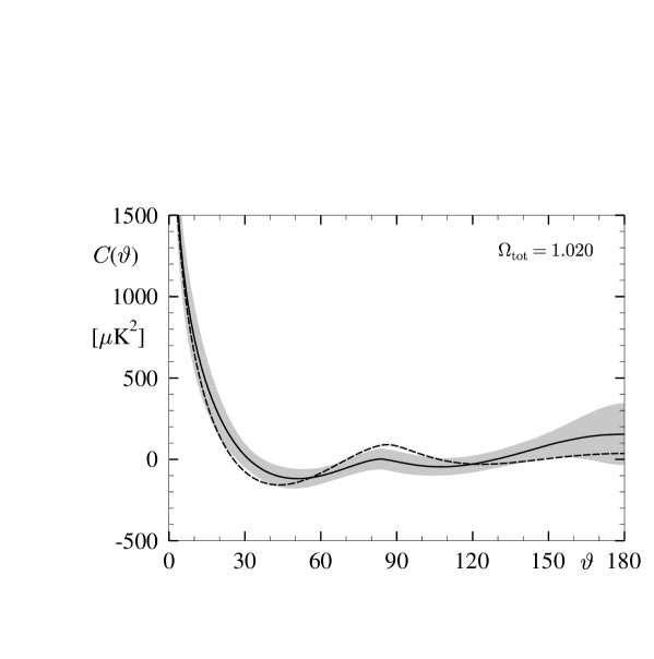
Figure 2: The SW contribution (44) of the temperature correlation function $C(\vartheta)$ is shown as a dashed curve for the dodecahedral space ${\cal D}$ for $\Omega_{\hbox{\scriptsize tot}}=1.020$. The solid curve shows the full result including the integrated Sachs-Wolfe and Doppler contribution. The $1\sigma$ deviation is shown as a grey band.

In our computations of the multipole moments $C_{l}$ for a given primordial realization, we use all eigenmodes with $\beta\leq 155$. Above this cut-off, we use in the mode summation up to $\beta=1501$ the conjecture (25) which describes the mean asymptotic behaviour. If only the modes below $\beta=155$ are used, the multipoles can only be calculated up to $l\simeq 15$. It is thus important for the calculation of $C(\vartheta)$ that the conjecture allows us to include higher multipoles.

Let us now come to the discussion of the CMB anisotropy in the Poincaré dodecahedral space, where, for simplicity, we assume that the dark energy is given by a cosmological constant with $\Omega_{\Lambda}:=\Omega_{\hbox{\scriptsize tot}}-\Omega_{\hbox{\scriptsize rad}}-\Omega_{\hbox{\scriptsize mat}}$. We have calculated the CMB anisotropy for different values of the cosmological parameters. Here we present only the results for $\Omega_{\hbox{\scriptsize bar}}=0.046$, $\Omega_{\hbox{\scriptsize mat}}=0.28$ and $h=0.70$.

Figure 3: The values of the $S(\rho)$ statistic (48) for the median values of $C(\vartheta)$ for the dodecahedral space for $\rho=60^{\circ}$ (full curve) and $\rho=20^{\circ}$ (dotted curve) in dependence on $\Omega_{\hbox{\scriptsize tot}}$ ($h=0.70$, $\Omega_{\hbox{\scriptsize mat}}=0.28$ and $\Omega_{\hbox{\scriptsize bar}}=0.046$).

To quantify the observed surprisingly low CMB anisotropy [4] on large scales, the $S$ statistic

$$S(\rho)\;=\;\int_{-1}^{\cos\rho}\big{|}C(\vartheta)\big{|}^{2}\;d\cos\vartheta$$ (48)

is discussed for the first year WMAP data in [28] for $\rho=60^{\circ}$, and it is found that only $0.3\%$ of the simulations based on the concordance model ri have lower values of $S(60^{\circ})$ than the observed value $S(60^{\circ})=1644$. Somewhat higher values of $S(60^{\circ})$ are obtained using other statistical methods and other sky masks in [56], but they are nevertheless surprisingly low. In figure 3 we show the values of $S(60^{\circ})$ (full curve) and $S(20^{\circ})$ (dotted curve) using the median values of $C(\vartheta)$ for the dodecahedral space ${\cal D}$ in dependence on $\Omega_{\hbox{\scriptsize tot}}$. One observes that the models with $\Omega_{\hbox{\scriptsize tot}}=1.017\dots 1.020$ give the lowest values for the large scale anisotropy.

Here and in the following calculations, the overall amplitude of the CMB anisotropy, i. e. the normalization constant $\alpha$ in (38), is fitted to the $C_{l}$ values of the first year WMAP data in the range $l\in[20,45]$. (Thus, the values cannot be directly compared to the ones in [35], where the amplitudes are scaled such that they match the $C_{4}$ value of WMAP exactly.)

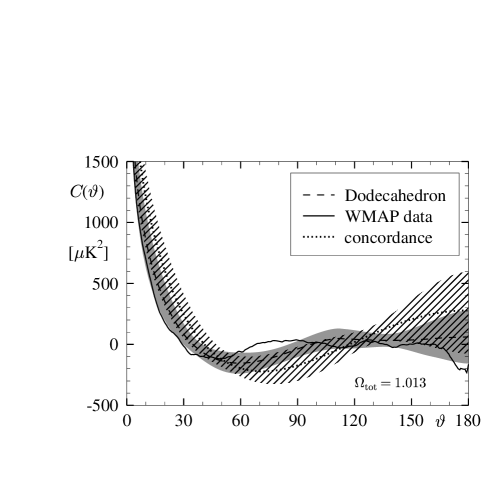
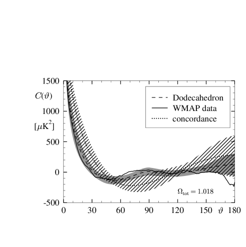
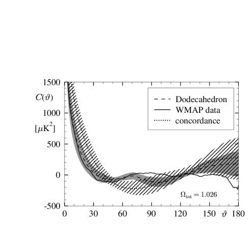
Figure 4: The temperature correlation function $C(\vartheta)$ for the dodecahedral topology for four values of $\Omega_{\hbox{\scriptsize tot}}$ for $h=0.70$, $\Omega_{\hbox{\scriptsize mat}}=0.28$ and $\Omega_{\hbox{\scriptsize bar}}=0.046$, the WMAP first year observation and the pl-concordance model (see description in the text).

In figure 4 the temperature correlation function $C(\vartheta)$ is shown for four values of $\Omega_{\hbox{\scriptsize tot}}$. The WMAP curve obtained from the LAMBDA home page http://lambda.gsfc.nasa.gov is shown as a full curve. The mean value of $C(\vartheta)$ for the pl-concordance model from the same home page is displayed as dotted curve. The $1\sigma$ deviation computed from 3000 HEALPix [57] simulations is shown as a shaded region. Finally, the mean value of $C(\vartheta)$ for the dodecahedral topology is shown as a dashed curved and the corresponding $1\sigma$ deviation is the grey region obtained from 500 simulations. In figure 4a), the value preferred in [35], i. e. $\Omega_{\hbox{\scriptsize tot}}=1.013$, is presented. One observes a general low anisotropy on large scales, however, a more than $1\sigma$ deviation from the WMAP values occurs in the range $\vartheta\in[60^{\circ},90^{\circ}]$. The WMAP data are much better described by models with $\Omega_{\hbox{\scriptsize tot}}=1.018$ and $\Omega_{\hbox{\scriptsize tot}}=1.019$ (figures 4b) and 4c)) as is also revealed by the better values for the $S$ statistic (compare figure 3). Only on the largest scales $\vartheta>170^{\circ}$, the models in figures 4b) and 4c) do not reproduce the large negative correlation obtained from the WMAP data. But without this blemish, the dodecahedral space describes in the considered $\Omega_{\hbox{\scriptsize tot}}$ range the observations down to the smallest scales, since the WMAP curve lies completely within the grey $1\sigma$ region. Finally, figure 4d) shows a model with $\Omega_{\hbox{\scriptsize tot}}=1.026$, where the $S$ statistic already deteriorates and consequently the agreement with the WMAP curve is also worse.

Figure 5: The angular power spectrum $\delta T_{l}^{2}$ for the dodecahedral topology (circles) for four values of $\Omega_{\hbox{\scriptsize tot}}$ for $h=0.70$, $\Omega_{\hbox{\scriptsize mat}}=0.28$ and $\Omega_{\hbox{\scriptsize bar}}=0.046$. The WMAP data are shown as diamonds with error bars, and the pl-concordance model is represented by the full curve.

In figures 5a) to 5d), the angular power spectrum $\delta T_{l}^{2}=l(l+1)C_{l}/(2\pi)$ is shown for the same values of $\Omega_{\hbox{\scriptsize tot}}$ as in figure 4. The WMAP data are represented by diamonds together with the $1\sigma$ error bars which do not include the cosmic variance. The mean values of $\delta T_{l}^{2}$ of the pl-concordance model (full curve) do not show the suppression of power at low values of $l$, but in contrast, increase there. The mean values of $\delta T_{l}^{2}$ for the dodecahedral space exhibit the suppression of power as observed by WMAP. A good agreement is observed exactly for those values of $\Omega_{\hbox{\scriptsize tot}}$ favored by the $S$ statistic and the correlation function $C(\vartheta)$. This behaviour is also revealed by figure 6 which shows the dependence on $\Omega_{\hbox{\scriptsize tot}}$ of the mean values of $\delta T_{2}^{2}$, $\delta T_{3}^{2}$ and $\delta T_{4}^{2}$ for the dodecahedral space ${\cal D}$. The lowest values of the quadrupole $\delta T_{2}^{2}$ are obtained near $\Omega_{\hbox{\scriptsize tot}}=1.017$. Furthermore, at $\Omega_{\hbox{\scriptsize tot}}=1.017$ the next multipole $\delta T_{3}^{2}$ matches the value obtained by WMAP almost perfectly.

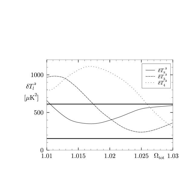
Figure 6: The mean values of $\delta T_{2}^{2}$ (solid curve), $\delta T_{3}^{2}$ (dashed curve) and $\delta T_{4}^{2}$ (dotted curve) are shown for the dodecahedral space ${\cal D}$ as a function of $\Omega_{\hbox{\scriptsize tot}}$. The lower horizontal line indicates the $\delta T_{2}^{2}$ value of WMAP and the upper one the corresponding value of $\delta T_{3}^{2}$.

The probability distribution of $\delta T_{2}^{2}$ and $\delta T_{3}^{2}$ obtained from sky simulations is for the pl-concordance model much broader than for the dodecahedral space. To emphasize this fact, figure 7 displays the distribution of $\delta T_{2}^{2}$ and $\delta T_{3}^{2}$ for $\Omega_{\hbox{\scriptsize tot}}=1.018$. The corresponding WMAP values are indicated by the vertical lines together with the $1\sigma$ error (vertical dark grey band). The shaded histogram shows the wide distribution of 3000 HEALPix simulations for the pl-concordance model. In contrast, a much more pronounced peak is revealed by the corresponding distribution of the dodecahedral space (light grey histogram). Furthermore, the peaks for $\delta T_{2}^{2}$ and $\delta T_{3}^{2}$ lie both within the $1\sigma$ error of the WMAP observation.

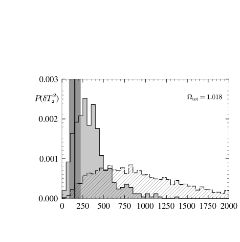
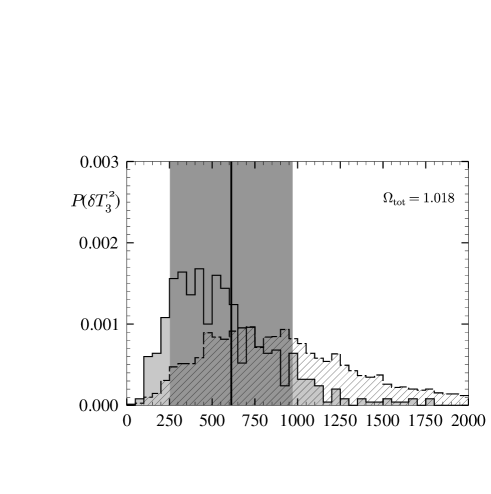
Figure 7: The probability distribution of $\delta T_{2}^{2}$ and $\delta T_{3}^{2}$ in $[\mu\hbox{K}^{2}]$ for $\Omega_{\hbox{\scriptsize tot}}=1.018$, $h=0.70$, $\Omega_{\hbox{\scriptsize mat}}=0.28$ and $\Omega_{\hbox{\scriptsize bar}}=0.046$ for the dodecahedral space (light grey histogram). The wide distribution of the pl-concordance model is shown as the shaded histogram. The WMAP values together with their $1\sigma$ error are indicated by the vertical line and the vertical grey band, respectively.

5 The circles-in-the-sky signature

A multi-connected space can reveal itself by the so-called circles-in-the-sky signature [8]. Consider an observer located at a given point $\vec{x}$ who measures the fluctuations of the CMB. The contribution to the CMB fluctuations due to the ordinary Sachs-Wolfe (SW) effect arises on a sphere around this observer having the radius $\tau_{\hbox{\scriptsize SLS}}$, i. e. at the so-called surface of last scattering (SLS) w. r. t. this observer. In the universal cover there are copies of this observer which have their own SLS’s which are centered at the copies of the observer. Those copies whose distance to the observer at $\vec{x}$ are smaller than $2\tau_{\hbox{\scriptsize SLS}}$ possess SLS’s which intersect the SLS of the observer sitting at $\vec{x}$. Since the intersection of two spheres is a circle, both the observer and its copy observe along this circle the same temperature fluctuations due to the ordinary Sachs-Wolfe effect. Since the observer and its copy have to be identified, there are two matching circles having the same radius on the sky and having an identical ordinary Sachs-Wolfe contribution. The integrated Sachs-Wolfe (ISW) contribution arises on the photon path from the SLS to the observer, see eq. (31). Since the two paths are not identified, their contribution is different on the matched circles. The two Doppler contributions are also different, since their velocity projections are different.

In the case of a flat toroidal universe, these different contributions to the temperature anisotropy are investigated in [58] with respect to the circles-in-the-sky signature, and it is found that the Doppler and the integrated Sachs-Wolfe contributions degrade the signature. That these two contributions play an important rôle also in the case of the dodecahedral topology, is demonstrated in figure 8. It shows the three competing contributions as computed from eq. (31) for the simply connected ${\cal S}^{3}$ (figure 8a)) and for the dodecahedral space ${\cal D}$ (figure 8b)). Here we use the conjecture (25) up to $\beta=4001$. For the SW contribution, see eq. (41). The most obvious difference between ${\cal D}$ and ${\cal S}^{3}$ is the suppression of power for small multipoles $\delta T_{l}$ in the case of ${\cal D}$ in comparison with ${\cal S}^{3}$. In the case of the dodecahedral space ${\cal D}$, the loss of power is so severe that for the quadrupole, the ISW dominates over the ordinary Sachs-Wolfe contribution. A further distinction between ${\cal S}^{3}$ and ${\cal D}$ is that $\delta T_{l}$ oscillates as a function of $l$ in the case of the multi-connected space even for the mean values of $\delta T_{l}$ which are considered here. With the exception of the smallest multipoles, the ordinary Sachs-Wolfe contribution dominates up to $l\lesssim 30$. However, even in this range the Doppler and the ISW contribution provide a significant fraction of the total temperature fluctuation. The ISW is most important for $l\lesssim 10$, whereas the Doppler contribution increases for $l\gtrsim 10$ to even larger values than the ISW, such that both contributions give together a large perturbation to the pure circles-in-the-sky signature.

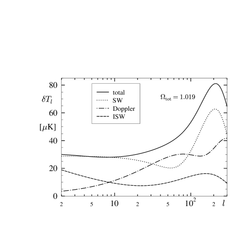
Figure 8: The three contributions to $\delta T_{l}$ are shown for the simply connected ${\cal S}^{3}$ (left) and the dodecahedral space ${\cal D}$ (right) calculated in the tight-coupling approximation for $\Omega_{\hbox{\scriptsize tot}}=1.019$, $h=0.70$, $\Omega_{\hbox{\scriptsize mat}}=0.28$ and $\Omega_{\hbox{\scriptsize bar}}=0.046$.

To emphasize this point, figure 9 shows the temperature fluctuation along two matched circles parameterized by the angle $\phi$ defined in (49) below. One observes in figure 9a) that the total temperature fluctuation $\delta T$ is not matched perfectly well. However, some rough similarities between both $\delta T$ curves are nevertheless visible. Whether such similarities occur sufficiently frequently by chance in the simply connected ${\cal S}^{3}$ model, such that the circles-in-the-sky signature is swamped, is discussed below. The different contributions to $\delta T$ are separately shown in figures 9b), 9c) and 9d). Even the ordinary Sachs-Wolfe contribution (figure 9b)) does not provide a perfect match which is due to the fact that the dipole contribution has been subtracted from the sky map analogously as it is done on the observational side. This destroys the perfect agreement due to the SW contribution. Conversely, if one would know the topological structure of the Universe, this would offer an opportunity to determine the dipole contribution due to the primordial fluctuations which is usually superseded by the Doppler shift due to our local motion. The Doppler and the ISW contributions are completely different for the two circles as seen in figures 9c) and 9d), respectively, for reasons described above.

Figure 9: The temperature fluctuation $\delta T$ is shown along two matched circles for $\Omega_{\hbox{\scriptsize tot}}=1.019$, $h=0.70$, $\Omega_{\hbox{\scriptsize mat}}=0.28$ and $\Omega_{\hbox{\scriptsize bar}}=0.046$. Panel a) displays $\delta T$ of the total temperature fluctuation along the two circles, obtained from the ordinary Sachs-Wolfe (SW), Doppler (Dop) and integrated Sachs-Wolfe (ISW) contribution, which are shown separately in panels b), c) and d), respectively.

As just discussed, for cosmological models near $\Omega_{\hbox{\scriptsize tot}}\simeq 1.02$, the ordinary Sachs-Wolfe contribution dominates for $l\lesssim 30$. The value $l=30$ corresponds to a scale $\theta\simeq\frac{180^{\circ}}{l}=6^{\circ}$. Thus the circles are blurred on scales below $\sim 6^{\circ}$. On larger scales, the integrated Sachs-Wolfe and the Doppler contribution lead to a modulation of matched circle structure.

For a quantitative search of matched circles in microwave sky maps, the quantity

$$\Sigma(\rho)\;:=\;\frac{\left<2\,\delta T_{a}(\pm\phi)\,\delta T_{b}(\phi+\rho)\right>}{\left<\delta T_{a}^{2}(\phi)+\delta T_{b}^{2}(\phi)\right>}$$ (49)

is introduced in [8]. (In [8], $\Sigma$ is called $S$, a name we avoid in the following in order to not confuse the reader with the previously discussed $S$ statistic.) Here $\delta T_{a}(\phi)$ and $\delta T_{b}(\phi)$ are the temperature fluctuations along two circles on the SLS with the same radius, and $\left<\right>:=\frac{1}{2\pi}\int_{0}^{2\pi}d\phi$. The angle $\rho$ describes the relative phase between the temperature fluctuations on the two circles and the plus/minus sign in the nominator allows for orientable as well as for non-orientable manifolds. The $\Sigma$ variable takes the value $\Sigma=+1$ in the case of a perfect correlation and $\Sigma=-1$ for anticorrelated temperature fluctuations.

Figure 10: The radius of the six matched circles is plotted as a function of $\Omega_{\hbox{\scriptsize tot}}$.

In [59] the $\Sigma$ test is applied to the first year data from WMAP and it is found that $\Sigma_{\hbox{\scriptsize max}}=\max_{\rho}\{\Sigma(\rho)\}$ does not show any spikes which would reveal a matched circle pair. The search is carried out for nearly back to back circles having a separation larger than $170^{\circ}$ and a radius larger than $25^{\circ}$. For $1.0091<\Omega_{\hbox{\scriptsize tot}}<1.0252$ (for $h=0.70$ and $\Omega_{\hbox{\scriptsize mat}}=0.28$) the Poincaré dodecahedron has in total 6 pairs of circles which are back to back, i. e. are separated by $180^{\circ}$. The radius of these circles increases with increasing $\Omega_{\hbox{\scriptsize tot}}$ as shown in figure 10. Above $\Omega_{\hbox{\scriptsize tot}}=1.0252$ there are at first 16 pairs, a number which increases further with increasing $\Omega_{\hbox{\scriptsize tot}}$, and below $\Omega_{\hbox{\scriptsize tot}}=1.0091$ there are none. The conclusion in [59] is thus that the topology of the Poincaré dodecahedron is excluded. However, in [60] a hint towards six pairs of circles having a radius of $11\pm 1^{\circ}$ is found which would correspond to $\Omega_{\hbox{\scriptsize tot}}=1.0094$ for our choice of $h$ and $\Omega_{\hbox{\scriptsize mat}}$.

Now we would like to discuss whether the Doppler and ISW contributions are significantly large enough in order to contaminate the SW contribution such that the circles-in-the-sky signature is hidden. We generate 500 sky maps for the dodecahedral space ${\cal D}$ using all modes up to $\beta\leq 155$ and compute for each of the six pairs of matched circles the value of $\Sigma_{\hbox{\scriptsize max}}$. In this way we get 3000 values for $\Sigma_{\hbox{\scriptsize max}}$ belonging to circle pairs including the SW, Doppler and ISW contribution. In addition, we obtain 3000 values for $\Sigma(\rho)$ where $\rho$ is not varied but instead is fixed to the value $\rho=36^{\circ}$ determined by the topology of ${\cal D}$. Due to the Doppler and the ISW contribution, the values of $\Sigma_{\hbox{\scriptsize max}}$ are usually larger than the correct values $\Sigma(\rho)$ for the matched pair of circles having $\rho=36^{\circ}$. This emphasizes that the contamination by the Doppler and the ISW contribution is so large that the $\Sigma_{\hbox{\scriptsize max}}$ statistic does in general not find the correct value of $\rho$. Furthermore, we compute also the corresponding values of $\Sigma_{\hbox{\scriptsize max}}$ for 500 simulations for the simply connected ${\cal S}^{3}$ universe with the same cut-off in $\beta$ and with the ring positions found in the dodecahedral space ${\cal D}$. Of course, the $\Sigma_{\hbox{\scriptsize max}}$ values of ${\cal S}^{3}$ do not correspond to a matched circle pair since ${\cal S}^{3}$ has none.

In figure 11, we compare the probability distribution of $\Sigma_{\hbox{\scriptsize max}}$ for ${\cal S}^{3}$ and ${\cal D}$ for the two values $\Omega_{\hbox{\scriptsize tot}}=1.011$ and $\Omega_{\hbox{\scriptsize tot}}=1.020$. These values are chosen in order to demonstrate the effect due to the size of the radii of the circles which are $25.4^{\circ}$ and $49.8^{\circ}$ for $\Omega_{\hbox{\scriptsize tot}}=1.011$ and $\Omega_{\hbox{\scriptsize tot}}=1.020$, respectively. The probability distributions shift to smaller values of $\Sigma_{\hbox{\scriptsize max}}$ with increasing radii. In figure 12, we again show the probability distribution of $\Sigma_{\hbox{\scriptsize max}}$ for ${\cal S}^{3}$ as in figure 11, but display for ${\cal D}$ the probability distribution of $\Sigma(\rho)$ with $\rho=36^{\circ}$. It is seen that the distribution for ${\cal D}$ has been shifted to smaller values of $\Sigma$, and thus the overlap of the distributions for ${\cal D}$ and ${\cal S}^{3}$ has increased.

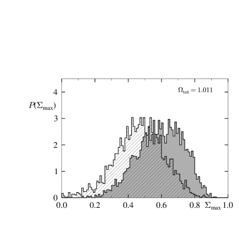
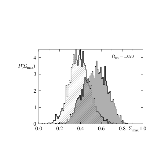
Figure 11: The probability distribution of $\Sigma_{\hbox{\scriptsize max}}$ for ${\cal S}^{3}$ (shaded histogram) and ${\cal D}$ (grey histogram) for $\Omega_{\hbox{\scriptsize tot}}=1.011$ in panel a) having a radius of $25.4^{\circ}$ and for $\Omega_{\hbox{\scriptsize tot}}=1.020$ in panel b) having a radius of $49.8^{\circ}$. The other cosmological parameters are $h=0.70$, $\Omega_{\hbox{\scriptsize mat}}=0.28$ and $\Omega_{\hbox{\scriptsize bar}}=0.046$ as usual.

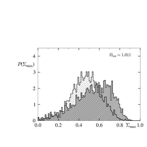
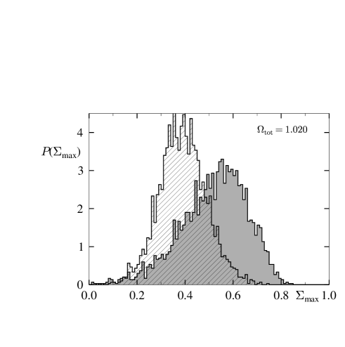
Figure 12: The probability distribution of $\Sigma_{\hbox{\scriptsize max}}$ for ${\cal S}^{3}$ (shaded histogram) as in figure 11 and of $\Sigma(\rho)$ for ${\cal D}$ with $\rho=36^{\circ}$ as determined by the topology of ${\cal D}$ (grey histogram) for $\Omega_{\hbox{\scriptsize tot}}=1.011$ in panel a) having a radius of $25.4^{\circ}$ and for $\Omega_{\hbox{\scriptsize tot}}=1.020$ in panel b) having a radius of $49.8^{\circ}$. The other cosmological parameters are as in figure 11.

Analysing a sky map which possesses no pairs of circles, one would obtain for randomly chosen circle pairs a distribution corresponding to the shaded histograms in figures 11 and 12. Now the aim is to find the six pairs of circles due to the dodecahedral topology. If there would be only the pure ordinary SW contribution, a value of $\Sigma_{\hbox{\scriptsize max}}=1$ would clearly stand out of the distribution due to ${\cal S}^{3}$. However, the Doppler and ISW contributions degrade this signal to the grey histograms in figures 11 and 12. Thus the six pairs would probably yield values of $\Sigma_{\hbox{\scriptsize max}}$ between 0.4 and 0.8 for $\Omega_{\hbox{\scriptsize tot}}=1.011$ and between 0.4 and 0.7 for $\Omega_{\hbox{\scriptsize tot}}=1.020$, and values of $\Sigma(\rho)$ between 0.3 and 0.75 for both values of $\Omega_{\hbox{\scriptsize tot}}$, respectively. In the case of an analysis of a real sky map, one would obtain many thousands of $\Sigma_{\hbox{\scriptsize max}}$ values which would not correspond to matched circles, i. e. having a probability distribution looking like that of ${\cal S}^{3}$. Embedded in this distribution, one would for the dodecahedron obtain six $\Sigma_{\hbox{\scriptsize max}}$ values corresponding to real matched circles. Because of the large overlap of both distributions, the signal of the six pairs of circles could easily be swamped. Thus there is a non-vanishing probability that the six pairs of matched circles can be overlooked in the sky maps. The search for matched circles is in addition made more difficult by the finite thickness of the SLS and the Sunyaev-Zeldovich effect, a possible systematic in the removal of foregrounds and further secondary effects which are not included in our analysis.

6 Discussion and Summary

Taking the WMAP value $\Omega_{\hbox{\scriptsize tot}}=1.02\pm 0.02$ as its face value, we conclude that the Universe is slightly positively curved and therefore necessarily spatially finite, since all spherical space forms possess this property. At present, the only way to decide on the particular topology realized in our Universe consists in studying a concrete space form and then compare its predictions with the observational data.

In this paper, we produce evidence in support of the hypothesis that the spatial structure of the Universe could be given by the Poincaré dodecahedral space ${\cal D}$, provided that the total energy density parameter $\Omega_{\hbox{\scriptsize tot}}$ is in the range $1.016\dots 1.020$. For the detailed comparison with the WMAP data, it was crucial that we could base our predictions for the CMB anisotropy upon a large number of vibrational modes of the Poincaré dodecahedron. Since the eigenfunctions of the Poincaré dodecahedron are not known analytically, they have to be computed numerically. Using the very efficient algorithm described in section 3, we could take in our calculations the first 10 521 eigenfunctions into account. In addition, we put forward the Conjecture (25) for the homogeneous spherical space forms. Combining the numerically computed eigenfunctions with the Conjecture, we were able to calculate the CMB multipoles in a broad range, see figures 5 and 8, covering the region of the large scale fluctuations. Fixing the cosmological parameters as $\Omega_{\hbox{\scriptsize bar}}=0.046$ and $\Omega_{\hbox{\scriptsize mat}}=0.28$, $h=70$, in agreement with the WMAP data, there are only two parameters left: the amplitude $\alpha$ of the scale-invariant Harrison-Zeld’ovich spectrum (38), and the density parameter $\Omega_{\hbox{\scriptsize tot}}>1$ or, equivalently, the curvature radius $R_{0}=\frac{c}{H_{0}}(\Omega_{\hbox{\scriptsize tot}}-1)^{-1/2}$. (The dark energy is identified with a cosmological constant with magnitude $\Omega_{\Lambda}:=\Omega_{\hbox{\scriptsize tot}}-\Omega_{\hbox{\scriptsize rad}}-\Omega_{\hbox{\scriptsize mat}}$.) The parameter $\alpha$ was obtained from a fit to the $C_{l}$ values as determined by WMAP in the range $l\in[20,45]$. (This differs from the normalization in [35], where $\alpha$ has been set to match the WMAP multipole with $l=4$ exactly, since higher multipoles could not be calculated in [35] due to the very limited number of available eigenfunctions.) Having fixed in this way all parameters except $\Omega_{\hbox{\scriptsize tot}}$, we studied the CMB multipoles and the temperature correlation function $C(\vartheta)$ for the dodecahedron as a function of $\Omega_{\hbox{\scriptsize tot}}$. One should keep in mind that we restricted the parameter space to the above values. Thus we cannot exclude that other choices could lead to different values for $\Omega_{\hbox{\scriptsize tot}}$ due to geometrical degeneracies.

As a quantitative measure of the quality of our theoretical predictions, we calculated the $S$ statistic (48) for the angles $\rho=60^{\circ}$ and $\rho=20^{\circ}$. The result is given as a function of $\Omega_{\hbox{\scriptsize tot}}$ in figure 3 and shows for this statistic the remarkable feature of pronounced minima at almost the same $\Omega_{\hbox{\scriptsize tot}}$ values, $\Omega_{\hbox{\scriptsize tot}}\in[1.016,1.020]$. In particular, figure 3 shows that the Poincaré dodecahedral universe leads for $\Omega_{\hbox{\scriptsize tot}}$ in the above range to a suppression of the CMB anisotropy at large scales in agreement with the WMAP data. This is also demonstrated in figure 4c), which shows the temperature correlation function $C(\vartheta)$, and in figures 5c) and 8b) showing the CMB power spectrum ($\Omega_{\hbox{\scriptsize tot}}=1.019$ is used in these figures). Figure 4c) demonstrates clearly that the dodecahedron model describes the WMAP data much better than the concordance model. At this point it is important to notice that the suppression of the CMB anisotropy at large scales occurring in the dodecahedron is neither obtained by fitting the theoretical curves to one of the first (suppressed) multipoles nor to the correlation function $C(\vartheta)$. Rather the suppression is due to the finiteness of the Universe in combination with a small volume of the dodecahedron, $V({\cal D})=\frac{\pi^{2}}{60}=0.16449\dots$, which is nicely illustrated in figure 8, where we compare the power spectra of the dodecahedron ${\cal D}$ and the simply connected ${\cal S}^{3}$, respectively. The structures seen in figures 5 and 8b) in the CMB power spectrum at multipoles $l\lesssim 20$, are mainly caused by the ordinary Sachs-Wolfe (SW) contribution (dotted curve in 8b)) whose analytic expression is given in eq. (41). The observed structures are a direct consequence of the discrete mode spectrum of ${\cal D}$ possessing large gaps at small wave numbers $\beta$, see eqs.(26) and (27).

The particularly striking suppression of the quadrupole and octopole is also exemplified by figure 7 which displays the probability distribution $P(\delta T_{l}^{2})$ ($l=2,3$) obtained from sky simulations. The probability distributions for the dodecahedron show pronounced peaks which overlap nicely with the $1\sigma$ band of the WMAP data. In contrast, the concordance model predicts much broader distributions producing large values for $\delta T_{2}^{2}$ and $\delta T_{3}^{2}$, seen also in figure 5.

Summarising the results discussed so far, it is fair to say that the Poincaré dodecahedral universe provides a natural explanation for the strange suppression of power at large scales as observed by COBE and WMAP, if $\Omega_{\hbox{\scriptsize tot}}$ is in the range $1.016\dots 1.020$, which solves “the mystery of missing fluctuations”. At this point we would like to emphasise that the good agreement of the Poincaré dodecahedral universe with the WMAP data does by no means exclude that there are other manifolds which lead to similar conclusions. Rather, it may well be that there exists a “topological degeneracy” in addition to the well-known “geometrical degeneracy” (see e. g. [24, 25]). Since the value $\Omega_{\hbox{\scriptsize tot}}=1.02\pm 0.02$ reported by the WMAP team depends on several priors and includes the $1\sigma$ deviation uncertainty only, there still exists the possibility of the Universe having negative curvature. In fact, e. g. the hyperbolic Picard space [26, 27] leads also to a suppression of the CMB fluctuations at large scales in agreement with the WMAP data.

There remains to detect a more direct signature of the dodecahedral topology. For this purpose, we have studied the circles-in-the-sky signature in section 5. The dodecahedral universe possesses exactly 6 matched circles with radii $42.7^{\circ}$ and $49.8^{\circ}$ for $\Omega_{\hbox{\scriptsize tot}}=1.016$ and $\Omega_{\hbox{\scriptsize tot}}=1.020$, respectively. If there would be only the ordinary Sachs-Wolfe contribution, one would predict an almost perfect matching of the circles. However, as it is seen in figure 8, there are important contributions from the integrated Sachs-Wolfe and the Doppler effect. The three contributions together destroy a perfect matching as is illustrated for a given circle pair in figure 9a). While the ordinary Sachs-Wolfe contribution displayed in figure 9b) shows the expected matching, the Doppler and the integrated Sachs-Wolfe contributions shown in figures 9c) and 9d), respectively, differ appreciably over the full angular range, and thus lead to the poor matching demonstrated in figure 9a).

The quantity $\Sigma(\rho)$, eq. (49), has been introduced for a search of matched circles in the microwave sky. Figures 11 and 12 display the probability distributions of $\Sigma_{\hbox{\scriptsize max}}$ and $\Sigma(36^{\circ})$, respectively. One observes broad distributions for both the dodecahedron ${\cal D}$ and the covering space ${\cal S}^{3}$. While the distribution for ${\cal D}$ is peaked at higher values of $\Sigma_{\hbox{\scriptsize max}}$ than the distribution for ${\cal S}^{3}$, the two distributions have a large overlap. Due to the contamination by the Doppler and integrated Sachs-Wolfe effect, the distribution for ${\cal D}$ has no peak at $\Sigma_{\hbox{\scriptsize max}}\simeq 1$, but rather gives for the most probable $\Sigma_{\hbox{\scriptsize max}}$ values at which the 6 matching circles are expected to be observed the interval $0.4\dots 0.8$.

In view of these complications, it seems that a search for matching circles in the first-year WMAP data is quite difficult, and thus the negative result reported in [8] does not yet allow to conclude that the dodecahedral model is excluded. We hope that the second-year WMAP data and the CMB measurements from the Planck satellite will improve the situation considerably such that we shall be able to decide about the topology of the Universe in the near future.

Let us close with a quotation from Einstein, who wrote in 1919 in describing the Universe of beings in a “finite and yet unbounded Universe” [61, 62]: “The great charm resulting from this consideration lies in recognition of the fact that the universe of these beings is finite and yet has no limits.”

References

References

- [1] A. Einstein, Sitzungsber. Preuß. Akad. Wiss. , 142 (1917).
- [2] K. Schwarzschild, Vierteljahrsschrift der Astron. Gesellschaft 35, 337 (1900).
- [3] G. F. Smoot et al., Astrophys. J. Lett. 396, L1 (1992).
- [4] C. L. Bennett et al., Astrophys. J. Supp. 148, 1 (2003), astro-ph/0302207.
- [5] M. Lachièze-Rey and J. Luminet, Physics Report 254, 135 (1995).
- [6] J. Levin, Physics Report 365, 251 (2002).
- [7] G. Hinshaw et al., Astrophys. J. Lett. 464, L25 (1996).
- [8] N. J. Cornish, D. N. Spergel, and G. D. Starkman, Class. Quantum Grav. 15, 2657 (1998).
- [9] A. G. Riess et al., Astron. J. 116, 1009 (1998).
- [10] S. Perlmutter et al., Astrophys. J. 517, 565 (1999).
- [11] E. Torbet et al., Astrophys. J. Lett. 521, L79 (1999).
- [12] A. D. Miller et al., Astrophys. J. Lett. 524, L1 (1999).
- [13] P. de Bernardis et al., Nature 404, 955 (2000).
- [14] S. Hanany et al., Astrophys. J. Lett. 545, L5 (2000), astro-ph/0005123.
- [15] A. Balbi et al., Astrophys. J. Lett. 545, L1 (2000), astro-ph/0005124.
- [16] J. R. Bond, D. Pogosyan, and T. Souradeep, Class. Quantum Grav. 15, 2671 (1998).
- [17] J. R. Bond, D. Pogosyan, and T. Souradeep, Phys. Rev. D 62, 043005 (2000), astro-ph/9912124.
- [18] J. R. Bond, D. Pogosyan, and T. Souradeep, Phys. Rev. D 62, 043006 (2000), astro-ph/9912144.
- [19] N. J. Cornish, D. Spergel, and G. Starkman, Phys. Rev. D 57, 5982 (1998).
- [20] R. Aurich, Astrophys. J. 524, 497 (1999).
- [21] N. J. Cornish and D. Spergel, Phys. Rev. D 62, 087304 (2000), astro-ph/9906401.
- [22] K. T. Inoue, K. Tomita, and N. Sugiyama, Mon. Not. R. Astron. Soc. 314, L21 (2000), astro-ph/9906304.
- [23] R. Aurich and F. Steiner, Mon. Not. R. Astron. Soc. 323, 1016 (2001), astro-ph/0007264.
- [24] R. Aurich and F. Steiner, Phys. Rev. D 67, 123511 (2003), astro-ph/0212471.
- [25] R. Aurich and F. Steiner, International Journal of Modern Physics D 13, 123 (2004), astro-ph/0302264.
- [26] R. Aurich, S. Lustig, F. Steiner, and H. Then, Class. Quantum Grav. 21, 4901 (2004), astro-ph/0403597.
- [27] R. Aurich, S. Lustig, F. Steiner, and H. Then, Phys. Rev. Lett. 94, 021301 (2005), astro-ph/0412407.
- [28] D. N. Spergel et al., Astrophys. J. Supp. 148, 175 (2003), astro-ph/0302209.
- [29] B. S. Mason et al., Astrophys. J. 591, 540 (2003).
- [30] T. J. Pearson et al., Astrophys. J. 591, 556 (2003).
- [31] C. L. Kuo et al., Astrophys. J. 600, 32 (2004).
- [32] M. Colless et al., Mon. Not. R. Astron. Soc. 328, 1039 (2001).
- [33] R. A. C. Croft et al., Astrophys. J. 581, 20 (2002).
- [34] J. Weeks, Notices of the American Mathematical Society 51, 610 (2004).
- [35] J. Luminet, J. R. Weeks, A. Riazuelo, R. Lehoucq, and J. Uzan, Nature 425, 593 (2003).
- [36] J. Uzan, A. Riazuelo, R. Lehoucq, and J. Weeks, Phys. Rev. D 69, 043003 (2004), astro-ph/0303580.
- [37] G. F. R. Ellis, Nature 425, 566 (2003).
- [38] R. Lehoucq, J. Weeks, J. Uzan, E. Gausmann, and J. Luminet, Class. Quantum Grav. 19, 4683 (2002), astro-ph/0205009.
- [39] M. Lachièze-Rey, Class. Quantum Grav. 21, 2455 (2004).
- [40] W. Threlfall and H. Seifert, Math. Annalen 104, 1 (1930).
- [41] W. Threlfall and H. Seifert, Math. Annalen 107, 543 (1932).
- [42] E. Schrödinger, Commentationes Pontificiae Academiae Scientiarium 2, 321 (1938).
- [43] E. Schrödinger, Physica 6, 899 (1939).
- [44] E. Schrödinger, Proc. Roy. Irish Academy 46A, 9 (1940).
- [45] E. Schrödinger, Proc. Roy. Irish Academy 46A, 25 (1940).
- [46] E. R. Harrison, Reviews of Modern Physics 39, 862 (1967).
- [47] L. F. Abbott and R. K. Schaefer, Astrophys. J. 308, 546 (1986).
- [48] J. A. Wolf, Spaces of constant curvature (Publish or Perish Boston, Mass., 1974), (Third edition).
- [49] W. P. Thurston, Three-dimensional geometry and topology (Princeton Univ. Press, Princeton, NJ, 1997).
- [50] E. Gausmann, R. Lehoucq, J. Luminet, J.-P. Uzan, and J. Weeks, Class. Quantum Grav. 18, 5155 (2001).
- [51] A. Ikeda, Kodai Math. J. 18, 57 (1995).
- [52] J. M. Bardeen, Phys. Rev. D 22, 1882 (1980).
- [53] R. Aurich and F. Steiner, Physica D 48, 445 (1991).
- [54] R. Aurich and J. Marklof, Physica D 118, 101 (1996).
- [55] W. Magnus, F. Oberhettinger, and R. P. Soni, Formulas and Theorems for the Special Functions of Mathematical Physics (Springer, Berlin, Heidelberg, New York, 1966), (Third enlarged edition).
- [56] G. Efstathiou, Mon. Not. R. Astron. Soc. 348, 885 (2004).
- [57] K. M. Górski, E. Hivon, and E. B. Wandelt, Analysis issues for large CMB data sets, in Proceedings of the MPA/ESO Cosmology Conference ”Evolution of Large-Scale Structure”, pp. 37–42, 1999, astro-ph/9812350, eds. A.J. Banday, R.S. Sheth and L. Da Costa, PrintPartners Ipskamp, NL (HEALPix web-site: http://www.eso.org/science/healpix).
- [58] A. Riazuelo, J. Uzan, R. Lehoucq, and J. Weeks, Phys. Rev. D 69, 103514 (2004), astro-ph/0212223.
- [59] N. J. Cornish, D. N. Spergel, G. D. Starkman, and E. Komatsu, Phys. Rev. Lett. 92, 201302 (2004), astro-ph/0310233.
- [60] B. F. Roukema, B. Lew, M. Cechowska, A. Marecki, and S. Bajtlik, Astron. & Astrophy. 423, 821 (2004), astro-ph/0402608.
- [61] A. Einstein, Über die spezielle und die allgemeine Relativitätstheorie. Gemeinverständlich (Friedr. Vieweg & Sohn, Braunschweig, 1919), (Vierte Auflage).
- [62] A. Einstein, Relativity. The Special and the General Theory (The Folio Society, London, 2004), authorized translation by R. W. Lawson.