Density Diagnostics of the Hot Plasma in AE Aquarii with XMM-Newton

Abstract

High resolution spectroscopy of AE Aquarii with the XMM-Newton RGS has enabled us to measure the electron number density of the X-ray-emitting hot plasma to be $\sim 10^{11}$ cm^-3 by means of intensity ratios of the He-like triplet of Nitrogen and Oxygen. Incorporating with the emission measure evaluated by the EPIC cameras, we have also found a linear scale of the plasma to be $\simeq 5\times 10^{10}$ cm. Both these values, obtained model-independently, are incompatible with a standard post-shock accretion column of a magnetized white dwarf, but are naturally interpreted as the plasma being formed through interaction between an accretion flow and the magnetosphere of the white dwarf. Our results provide another piece of evidence of the magnetic propeller effect being at work in AE Aqr.

1 Introduction

AE Aqr is a close binary system composed of a magnetized white dwarf rotating at a period of $33.08$ s (Patterson, 1979) and a Roche-lobe filling K3IV secondary star orbiting at a period of 9.88 h (Welsh, Horne, & Gomer, 1993). The masses of the primary and the secondary are reported to be $M_{1}=0.79\pm 0.16M_{\odot}$ and $M_{2}=0.50\pm 0.10M_{\odot}$ (Casares, Mouchet, Martinez-Pais, & Harlaftis, 1996), and the orbital semi-major axis length is $a=1.8\times 10^{11}$ cm.

AE Aqr has been known as one of the most enigmatic magnetic Cataclysmic Variables (mCVs) on various aspects, including large optical flares and flickering (Patterson, 1979), large radio flares (Bastian, Beasley, & Bookbinder, 1996), TeV $\gamma$-ray emissions (Meintjes et al., 1994) and so on. Although the orbital period of this long predicts existence of an accretion disk, an optical spectrum of AE Aqr does not seem as such, but only shows a broad single-peaked H$\alpha$ emission whose centroid velocity was found to lag behind the white dwarf orbit by some 70^∘ (Welsh, Horne, & Gomer, 1993). Hard X-ray emissions from magnetic CVs (mCVs) originate from the post-shock plasma that takes place close to the white dwarf surface in the accretion column. Although the plasma temperature is a few tens of keV in general (Ezuka & Ishida, 1999; Ishida & Fujimoto, 1995), that of AE Aqr is measured to be as low as $\sim 3$ keV (Eracleous, 1999; Choi, Dotani, & Agrawal, 1999). All these results, together with discovery of a steady spin-down of the white dwarf at a rate $\dot{P}=5.64\times 10^{-14}$ s s^-1 (de Jager, Meintjes, O’Donoghue, & Robinson, 1994), lead Wynn, King, & Horne (1997) to draw a picture that the accreting matter from the secondary trapped at the magnetosphere does not accrete onto the white dwarf but is expelled from the binary owing to magnetic torque (Welsh, Horne, & Gomer, 1998; Ikhsanov, 2001). This is so-called the magnetic propeller effect.

In this paper, we present new observational results that strongly indicate the magnetic propeller being at work in AE Aqr, by means of a model-independent density diagnostics with the He-like triplet of Nitrogen and Oxygen fully resolved by the XMM-Newton RGS for the first time.

2 Observations

AE Aqr was observed with XMM-Newton (Jansen et al., 2001) on 2001 November 7–8. The observation log is given in Table 1. The entire observation consists of two parts. During the former $\sim$10 ks, both the EPIC pn (Strüder et al., 2001) and MOS (Turner et al., 2001) had been switched off. The RGS (den Herder et al., 2001), on the other hand, had been normally operated throughout the observation. As a result, 27 ks data are available for the RGS and 17 ks for the EPIC pn/MOS. In Fig. 1 shown are the light curves of pn, MOS1, and RGS1.

For the data reduction, we use the SAS version 6.0.0. We adopt circular apertures of $54.\!\!^{\prime\prime}7$ and $50.\!\!^{\prime\prime}6$ in radius as the source photon integration region for pn and MOS, respectively. The background photons are accumulated from concentric annuli, being set out of the source regions, with three times larger outer radii. Source photons are somewhat piled up in the pn data especially during the flare. We thus have excluded the central circular region with a diameter of 16^′′ from the analysis of pn data.

3 Data Analysis

3.1 The EPIC Spectra

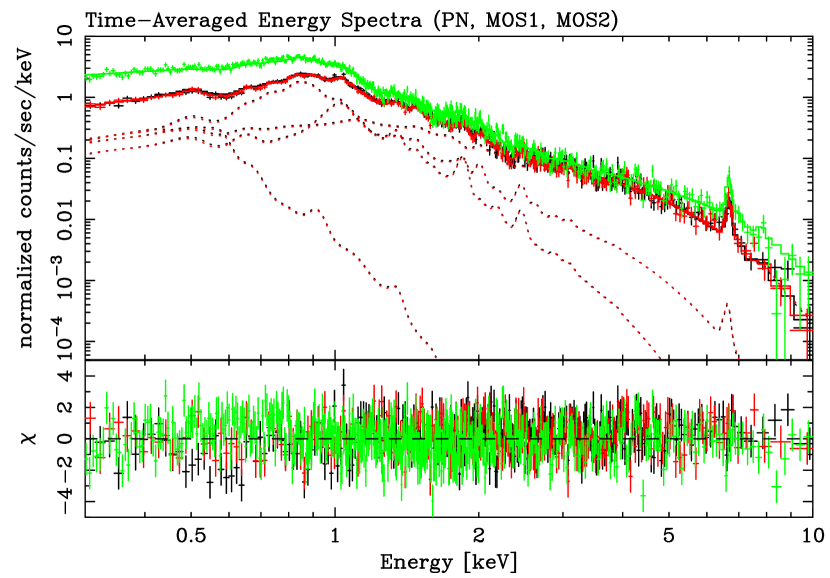
Figure 2: The averaged spectra of EPIC pn (green), MOS1 (black) and MOS2 (red) overlaid with the best-fit four temperature vmekal model as the histograms. The model components are drawn with the dotted lines for MOS1 and MOS2. See table 2 for the best-fit parameters.

The time-averaged energy spectra extracted separately from the MOS and pn data are shown in Fig. 2. A number of K$\alpha$ emission lines of H-like and/or He-like Ne, Mg, Si, S, and Fe can be recognized. Coexistence of these lines indicate that the X-ray emission originates from a multi-temperature optically thin thermal plasma (Choi, Dotani, & Agrawal, 1999; Eracleous, 1999). We thus have adopted a multi-temperature vmekal model (Mewe, Kaastra, & Liedahl, 1995) to fit these spectra. We have added a new temperature component one by one until the addition of a new component does not improve the fit significantly on the basis of F-test. To this end, we have arrived at a four temperature vmekal model with common elemental abundances undergoing photoelectric absorption with a common hydrogen column density. The best-fit parameters are listed in Table 2. Emission measures of the four continuum components with the temperatures of 0.14, 0.59, 1.4, and 4.6 keV are $1.3$, $3.6$, $2.7$, and $5.3\times 10^{53}\mathrm{cm}^{-3}$, and $1.29\times 10^{54}\mathrm{cm}^{-3}$ in total, for the assumed distance of 100 pc (Welsh, Horne, & Oke, 1993). The highest temperature $kT=4.6$ keV is considerably lower than any other mCVs. Also, the fluorescent neutral iron K$\alpha$ emission line at 6.40 keV ubiquitous among mCVs (Ezuka & Ishida, 1999) is absent. The upper limit of its equivalent width is obtained to be $<88$ eV. Thanks to a large effective area of XMM-Newton, the abundances of the elements from N to Ni are obtained. They are generally sub-solar (Anders & Grevesse, 1989), except for N which is more than three times the solar value.

3.2 Line Intensities from RGS Spectra

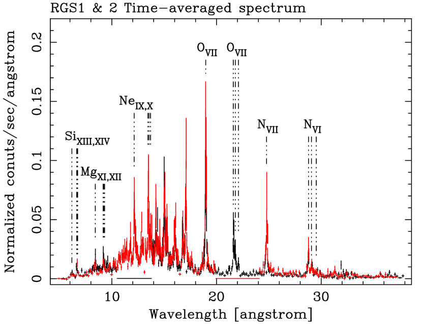
Figure 3: The RGS spectra averaged over the entire 27 ks exposure. The black and red points represent the data from RGS1 and RGS2, respectively. Identifications of the H-line and He-like K$\alpha$ lines of N through Si are shown with dotted-dashed line. The other unidentified lines are mainly those associated with Fe-L transitions.

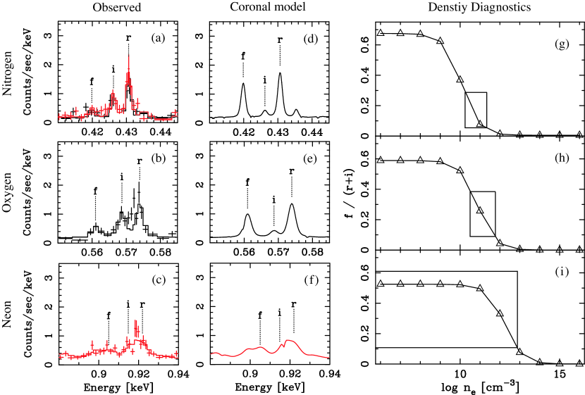
Figure 4: Density diagnostics by means of the He-like triplet. Panels of observed and coronal limit spectra around the He-like triplet, and the density diagnostics are arranged from left to right columns. The cases of Nitrogen, Oxygen, and Neon are arranged from upper to lower raws. Black and red data points and histograms are from RGS1 and RGS2. The relative intensities of the intercombination (marked with ‘i’) and forbidden (marked with ‘f’) lines are undoubtedly inverted for N and O. In the panels (g)-(i), comparisons of theoretical curves of the intensity ratio $f/(r+i)$ versus the electron density $n_{\rm e}$ with the observed intensity ratio. In drawing the theoretical curves we have used the plasma code spec (Kaastra, Mewe, & Nieuwenhuijzen, 1996) at the ionization temperatures $kT_{i}$ of 0.15, 0.30, and 0.34 keV for N, O, and Ne obtained from the intensity ratio between Ly$\alpha$ and $r$.

In Fig. 3 we have shown the RGS spectra. The K$\alpha$ emission lines from Nitrogen through Silicon in the H-like and/or He-like ionization states can easily be recognized. Figure 4 (a)-(c) are blow-up of energy bands of the He-like triplets of N, O, and Ne. In the next column shown are the spectra predicted by the best-fit four temperature vmekal model (table 2), being convolved by the RGS1 1st order response function. Note that the vmekal model represents emission spectrum from a thermal plasma in the low density coronal limit. One can easily see, for N and O, that the intensity of the intercombination increases from the coronal limit by consumption of the forbidden. This behavior is interpreted as a high density effect; if the electron density exceeds a certain critical value inherent in each element, one of the two electrons excited to the upper level of the forbidden line (${}^{3}\mathrm{S}_{1}$) is further pumped by another impact of a free electron up to the higher level ${}^{3}\mathrm{P}_{2,\,1}$, and is then relaxed by radiating the intercombination line. The relative intensities of the intercombination and forbidden lines can therefore be utilized as a density diagnostics (Gabriel & Jordan, 1969; Pradhan & Shull, 1981).

In order to evaluate the electron number density $n_{\mathrm{e}}$, we begin with evaluating intensities of the He-like triplets. For this, we utilize the four temperature vmekal model that provides the best-fit to the EPIC pn and MOS spectra. We have fixed the hydrogen column density and the four temperature at the values in table 2 and the relative normalizations of the four continuum components. The abundances are also fixed at the best-fit values, except for an element to be used as a density diagnostic, for which the abundance is set equal to zero, and instead, four Gaussians are added, representing the He-like triplet and the Ly$\alpha$ line. The line intensities thus obtained for N, O, and Ne are summarized in table 3, and the best-fit results are displayed in Fig. 4 (a)-(c) as the histograms. The ionization temperature $kT_{i}$ calculated from the intensity ratio between the Ly$\alpha$ and $r$ are obtained to be 0.16, 0.30, and 0.34 keV for N, O, and Ne, respectively.

Given the line intensities of the triplets, we have carried out density diagnostics by means of the intensity ratio $f/(r+i)$. In Fig. 4 (g)-(i) shown are theoretical curves of the ratio $f/(r+i)$ versus the electron density, which is calculated by means of the plasma code spex (Kaastra, Mewe, & Nieuwenhuijzen, 1996) at the ionization temperature $kT_{i}$ of each element. In each panel we have also drawn a range of the intensity ratio allowed from the data and the resultant density range as a box. The electron densities are obtained to be $1.4\times 10^{10}-1.3\times 10^{11}\mathrm{cm}^{-2}$, $4.0\times 10^{10}-6.8\times 10^{11}\mathrm{cm}^{-2}$, and $<9.3\times 10^{12}\mathrm{cm}^{-2}$ for N, O, and Ne, respectively. As a crude approximation, the electron number density of the plasma is $n_{\rm e}\simeq 10^{11}{\rm cm}^{3}$.

4 Discussion and Conclusion

It is of great importance to note that the resultant density $n_{\rm e}\simeq 10^{11}{\rm cm}^{3}$ is smaller by several orders of magnitude than the conventional estimate in the post-shock accretion column of mCVs: $n_{\rm e}\simeq 10^{16}{\rm cm}^{-3}$ (Frank, King, & Raine, 2002). Moreover, combined with the emission measure $EM=1.3\times 10^{54}{\rm cm}^{-3}$ obtained with the EPIC pn/MOS (§ 3.1), the linear scale of the plasma is evaluated to be $\ell_{\mathrm{p}}=(EM/n_{\rm e}^{2})^{1/3}\simeq 5\times 10^{10}$ cm, which is much larger than a radius of a typical white dwarf and rather close to the orbital scale. We thus conclude that the optically thin hot plasma in AE Aqr does not accrete onto the white dwarf but rather spreads over the orbit of the binary. Note that this conclusion is derived simply on the basis of widely approved atomic physics, and hence, is free from any specific model.

It is known, however, that photo-excitation due to UV radiation can also pump ${}^{3}\mathrm{S}_{1}$ electron up to ${}^{3}{\rm P}_{2,\,1}$, thereby affecting the density diagnostics. Although there is no evidence of accretion disk in AE Aqr (Welsh, Horne, & Gomer, 1993) and the secondary star is a late type K3 subgiant, the white dwarf can be a source of the photo-excitation, the emission spectrum of which is reported to be a blackbody with a temperature of $T_{\rm r}=26,000$ K (Welsh, 1999). The photo-excitation rate of such a white dwarf from the initial state $i=\;^{3}\mathrm{S}_{1}$ to the final state $j=\;^{3}{\rm P}_{2,\,1}$ is

$$\Gamma_{ij}(T_{\rm r})\;=\;\frac{\pi e^{2}}{m_{\rm e}c}\,f_{ij}\cdot W\cdot\frac{\pi B_{\nu}(T_{\rm r})}{h\nu}$$ (1)

(Porquet et al., 2001; Mauche, 2002) where $f_{ij}$ is the effective oscillator strength of photo-excitation which is 0.03574 (Nahar & Pradhan, 1999), and $W$ is a geometrical dilution factor to be taken here as $(R_{wd}/\ell_{\rm p})^{2}$ where $R_{wd}$ is the radius of the white dwarf. On the other hand, the collisional excitation rate to be compared with $\Gamma_{ij}$ is $n_{\rm e}q_{ij}$, where,

$$q_{ij}(T_{\rm e})\;=\;\frac{8.63\times 10^{-6}}{\omega_{i}\,T_{\rm e}^{1/2}}\,e^{-E_{ij}/kT_{\rm e}}\gamma_{ij}(T_{\rm e})\;\;\;{\rm[\,cm^{3}\;s^{-1}\,]}$$ (2)

is the rate coefficient of the electron impact excitation (Mewe & Schrijver, 1978). In this equation, $\omega_{i}(=3)$ is the statistical weight of the lower level, $E_{ij}$ is the energy difference between the two levels, and $\gamma_{ij}$ is the Maxwellian-averaged collision strength which is tabulated as a function of $T_{\rm e}$ in Pradhan, Norcross, & Hummer (1981). Adopting $T_{i}$ listed in table 3 as $T_{\rm e}$, we compared eqs. (1) and (2) and obtained $\Gamma_{ij}\simeq 0.07\,n_{\rm e}q_{ij}$ for both N and O. Hence, the photo-excitation effect can be neglected in the first order approximation.

We remark that the density obtained in § 3.2 should be treated as an upper limit, in the case that the UV radiation is stronger than the estimation above. Even if so, the conclusion above need not to be changed because a lower density, and hence, a larger geometrical scale are required for the plasma.

The low density and the large scale of the plasma naturally lead us to invoke the magnetic propeller model, in which blobby accreting matter originally following a ballistic trajectory from the inner Lagrangian point is gradually penetrated by the magnetic field of the white dwarf, and is finally blown out of the binary due to interaction with the rapid rotating white dwarf magnetosphere (Wynn, King, & Horne, 1997). The magnetic propeller model is advantageous in explaining various characteristics of AE Aqr, such as the spin down of the white dwarf, the velocity modulation of H$\alpha$ line. The low plasma temperature compared with other mCVs can be attributed to a halfway release of the gravitational potential energy of accreting matter down to the magnetosphere. We believe that the density diagnostics presented here add another piece of evidence to support the magnetic propeller effect being at work in AE Aqr.

Welsh, Horne, & Gomer (1998) estimated that the velocity of the out-flowing plasma can be as high as several hundred km at most. If so, a Doppler shift of the N and O lines may be detected through phase-resolved spectral analysis. We thus have made RGS spectra of the first and second flares separately, during the time interval of 3,000-8,500 s and 19,000-26,000 s in Fig. 1, respectively, and evaluated the central energy of Oxygen Ly$\alpha$. The result is negative with the line central energies of $653.4\pm 0.5$ eV and $653.4\pm 0.4$ eV, respectively, which are fully consistent with the laboratory value. We have further split the data of the second flare into evenly segregated three pieces, but the central energy distributes in the range 653.2-653.4 eV. Note, however, that we have obtained a finite value for a 1-$\sigma$ line width of $2.4\pm 0.6$ eV and $1.7\pm 0.6$ eV for the first and second flares, respectively, which are larger than the natural width ($\sim 0.001$ eV) or the thermal velocity of Oxygen ion ($\sim 70$ km s^-1 or $\sim 0.2$ eV estimated from $kT_{i}=0.3$ keV). Since the ionization temperature of Oxygen is lower than the highest temperature of the plasma (table 2) by an order of magnitude, and also from the fact $\ell_{\rm p}\simeq 5\times 10^{10}$ cm, the Oxygen Ly$\alpha$ line emanates from a region far out of the magnetosphere where the velocity collimation is already dissolved.

In order to finally confirm the magnetic propeller effect being at work in AE Aqr, it is important to detect a bulk velocity shift of an emission line expected from the plasma flow in the vicinity of the magnetosphere. Since the highest temperature of $\sim 5$ keV, we expect this can be done by the iron K$\alpha$ line with the Astro-E2 XRS.

Table 1: Observation Log

Obs. ID	Instrument	Data Mode	Obs. Start (UT)	Obs. End (UT)	Exp.(s)
0111180601	RGS1	Spectroscopy	2001-11-07 20:06:35	2001-11-07 22:53:33	10018
	RGS2	Spectroscopy	2001-11-07 20:06:35	2001-11-07 22:53:28	10013
0111180201	MOS1	Large Window	2001-11-07 23:06:36	2001-11-08 03:42:09	16533
	MOS2	Large Window	2001-11-07 23:06:35	2001-11-08 03:42:08	16533
	pn	Full Frame	2001-11-07 23:45:53	2001-11-08 03:38:17	13910
	RGS1	Spectroscopy	2001-11-07 23:00:19	2001-11-08 03:45:39	17120
	RGS2	Spectroscopy	2001-11-07 23:00:19	2001-11-08 03:45:36	17117

Table 2: The best-fit parameters of the 4 temperature vmekal model being fit to EPIC pn and MOS spectra

Parameter	Value	Element	Abundance
$N_{\rm H}$ $(10^{20}\mathrm{cm^{-2}})$	$3.59^{+1.47}_{-1.20}$	N	$3.51^{+0.92}_{-0.81}$
$kT_{1}~{}(\mathrm{keV})$	$4.60^{+0.60}_{-0.47}$	O	$0.74^{+0.17}_{-0.23}$
$kT_{2}~{}(\mathrm{keV})$	$1.21^{+0.13}_{-0.08}$	Ne	$0.43^{+0.28}_{-0.25}$
$kT_{3}~{}(\mathrm{keV})$	$0.59^{+0.02}_{-0.02}$	Mg	$0.70^{+0.15}_{-0.14}$
$kT_{4}~{}(\mathrm{keV})$	$0.14^{+0.05}_{-0.02}$	Si	$0.81^{+0.15}_{-0.12}$
$N_{1}$ $(10^{-3})$	$4.45^{+0.41}_{-0.44}$	S	$0.73^{+0.20}_{-0.18}$
$N_{2}$ $(10^{-3})$	$2.25^{+0.52}_{-0.51}$	Ar	$0.21~{}(<0.89)$
$N_{3}$ $(10^{-3})$	$3.04^{+0.47}_{-0.41}$	Ca	$0.19~{}(<1.11)$
$N_{4}$ $(10^{-3})$	$1.07^{+0.64}_{-0.37}$	Fe	$0.47^{+0.07}_{-0.06}$
$N_{\rm pn}/N_{\rm MOS}$	$1.08^{+0.01}_{-0.01}$	Ni	$1.27^{+0.57}_{-0.50}$
$\chi^{2}_{\nu}$ (d.o.f.)	1.22 (992)

Note. — All the errors are at the 90 % confidence level.

Table 3: Intensities of Ly$\alpha$ and He-like triplet of Nitrogen, Oxygen and Neon with RGS

	Nitrogen		Oxygen		Neon
	Energy	Norm	Energy	Norm	Energy	Norm
Ly$\alpha$	0.50032	$1.85^{+0.21}_{-0.21}$	0.65348	$3.63^{+0.34}_{-0.35}$	1.0215	$0.90^{+0.23}_{-0.23}$
$r$	0.43065	$0.97^{+0.17}_{-0.17}$	0.57395	$1.06^{+0.22}_{-0.23}$	0.92195	$0.65^{+0.22}_{-0.22}$
$i$	0.42621	$0.57^{+0.17}_{-0.17}$	0.56874	$0.85^{+0.22}_{-0.22}$	0.91481	$0.24^{+0.21}_{-0.21}$
$f$	0.41986	$0.26^{+0.14}_{-0.13}$	0.56101	$0.37^{+0.17}_{-0.18}$	0.90499	$0.32^{+0.18}_{-0.18}$
$kT_{i}$	$0.16\pm 0.02$		$0.30^{+0.04}_{-0.03}$		$0.34^{+0.09}_{-0.07}$
$\chi^{2}_{\nu}$ (d.o.f.)	1.36 (115)		1.14 (69)		1.21 (63)

Note. — All the errors are at the 90 % confidence level.

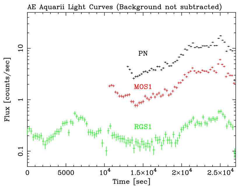
Figure 1: The light curves of EPIC pn and MOS1 in the band 0.2–15 keV, and RGS1 in the band 5–35 Åwith a bin size of 256 sec. The source integration region is a circle with a radius of $57.\!\!^{\prime\prime}4$ and $50.\!\!^{\prime\prime}6$ for pn and MOS1, respectively. The RGS1 light curve is created with the 1st order photons.

References

- Anders & Grevesse (1989) Anders, E. & Grevesse, N. 1989, Geochim. Cosmochim. Acta, 53, 197
- Bastian, Beasley, & Bookbinder (1996) Bastian, T. S., Beasley, A. J., & Bookbinder, J. A. 1996, ApJ, 461, 1016
- Casares, Mouchet, Martinez-Pais, & Harlaftis (1996) Casares, J., Mouchet, M., Martinez-Pais, I. G., & Harlaftis, E. T. 1996, MNRAS, 282, 182
- Choi, Dotani, & Agrawal (1999) Choi, C., Dotani, T., & Agrawal, P. C. 1999, ApJ, 525, 399
- de Jager, Meintjes, O’Donoghue, & Robinson (1994) de Jager, O. C., Meintjes, P. J., O’Donoghue, D., & Robinson, E. L. 1994, MNRAS, 267, 577
- den Herder et al. (2001) den Herder, J. W., et al. 2001, A&A, 365, L7
- Eracleous (1999) Eracleous, M. 1999, ASP Conf. Ser. 157: Annapolis Workshop on Magnetic Cataclysmic Variables, 343
- Ezuka & Ishida (1999) Ezuka, H. & Ishida, M. 1999, ApJS, 120, 277
- Frank, King, & Raine (2002) Frank, J., King, A., & Raine, D. J. 2002, Accretion Power in Astrophysics: Third Edition, by Juhan Frank, Andrew King, and Derek J. Raine. Cambridge University Press, 2002, 398 pp., Chapter 6
- Gabriel & Jordan (1969) Gabriel, A. H. & Jordan, C. 1969, MNRAS, 145, 241
- Ikhsanov (2001) Ikhsanov, N. R. 2001, A&A, 374, 1030
- Ishida & Fujimoto (1995) Ishida, M. & Fujimoto, R. 1995, ASSL Vol. 205: Cataclysmic Variables, 93
- Jansen et al. (2001) Jansen, F., et al. 2001, A&A, 365, L1
- Kaastra, Mewe, & Nieuwenhuijzen (1996) Kaastra, J. S., Mewe, R., & Nieuwenhuijzen, H. 1996, UV and X-ray Spectroscopy of Astrophysical and Laboratory Plasmas : Proceedings of the Eleventh Colloquium on UV and X-ray … held on May 29-June 2, 1995, Nagoya, Japan. Edited by K. Yamashita and T. Watanabe. Tokyo : Universal Academy Press, 1996. (Frontiers science series ; no. 15)., p.411, 411
- Mauche (2002) Mauche, C. W. 2002, ASP Conf. Ser. 261: The Physics of Cataclysmic Variables and Related Objects, 113
- Meintjes et al. (1994) Meintjes, P. J., de Jager, O. C., Raubenheimer, B. C., Nel, H. I., North, A. R., Buckley, D. A. H., & Koen, C. 1994, ApJ, 434, 292
- Mewe, Kaastra, & Liedahl (1995) Mewe, R., Kaastra, J. S., & Liedahl, D. A. 1995, Legacy, 6, 16
- Mewe & Schrijver (1978) Mewe, R. & Schrijver, J. 1978, A&A, 65, 99
- Nahar & Pradhan (1999) Nahar, S. N. & Pradhan, A. K. 1999, A&AS, 135, 347
- Patterson (1979) Patterson, J. 1979, ApJ, 234, 978
- Porquet et al. (2001) Porquet, D., Mewe, R., Dubau, J., Raassen, A. J. J., & Kaastra, J. S. 2001, A&A, 376, 1113
- Pradhan, Norcross, & Hummer (1981) Pradhan, A. K., Norcross, D. W., & Hummer, D. G. 1981, ApJ, 246, 1031
- Pradhan & Shull (1981) Pradhan, A. K. & Shull, J. M. 1981, ApJ, 249, 821
- Strüder et al. (2001) Strüder, L., et al. 2001, A&A, 365, L18
- Turner et al. (2001) Turner, M. J. L., et al. 2001, A&A, 365, L27
- Welsh (1999) Welsh, W. F. 1999, ASP Conf. Ser. 157: Annapolis Workshop on Magnetic Cataclysmic Variables, 357
- Welsh, Horne, & Gomer (1998) Welsh, W. F., Horne, K., & Gomer, R. 1998, MNRAS, 298, 285
- Welsh, Horne, & Gomer (1993) Welsh, W. F., Horne, K., & Gomer, R. 1993, ApJ, 410, L39
- Welsh, Horne, & Oke (1993) Welsh, W. F., Horne, K., & Oke, J. B. 1993, ApJ, 406, 229
- Wynn, King, & Horne (1997) Wynn, G. A., King, A. R., & Horne, K. 1997, MNRAS, 286, 436