A Simultaneous RXTE and XMM-Newton Observation of the Broad-Line Radio Galaxy 3C 111

Abstract

We present the results of simultaneous XMM-Newton and RXTE observations of the Broad-Line Radio Galaxy 3C 111. We find that the Compton reflection bump is extremely weak, however, broad residuals are clearly present in the spectrum near the Fe K${\rm\alpha}\,$emission line region. When fitted with a Gaussian emission line, the feature has an equivalent width of 40–100 eV and full-width at half maximum of greater than 20,000$\;{\rm km\;s^{-1}}$, however the exact properties of this weak line are highly dependent upon the chosen continuum model. The width of the line suggests an origin in the inner accretion disk, which is, however, inconsistent with the lack of Compton reflection. We find that much of the broad residual emission can be attributed to continuum curvature. The data are consistent with a model in which the primary powerlaw continuum is reprocessed by an accretion disk which is truncated as small radii. Alternatively, the primary source could be partially covered by a dense absorber. The latter model is less attractive than the former because of the small inclination angle of the jet of 3C 111 to the line of sight. We consider it likely that the curved continuum of the partial covering model is fortuitously similar to the continuum shape of the reprocessing model. In both models, the fit is greatly improved by the addition of an unresolved Fe K${\rm\alpha}\,$emission line, which could arise either in a Compton-thin obscuring torus or dense clouds lying along the line of sight. We also find that there are unacceptable residuals at low energies in the MOS data in particular, which were modeled as a Gaussian with an energy of $\sim 1.5$  keV; we attribute these residuals to calibration uncertainties of the MOS detectors.

1. INTRODUCTION

In the early 1990s, observations with the Ginga satellite revealed that the spectra of many Seyfert 1 galaxies contain an Fe K${\rm\alpha}\,$emission line, with an equivalent width ($EW$) of 100–300 eV, as well as a hard excess above 10 keV, relative to the simple powerlaw spectrum fitted over the interval from 2–8 keV (Pounds et al, 1990; Piro, Yamauchi, & Matsuoka, 1990; Matsuoka et al., 1990; Nandra & Pounds, 1994). These features were readily interpreted as signatures of the reprocessing of the primary X-ray continuum emission by nearby Compton-thick material, such as the accretion disk or the obscuring torus (see, e.g. Lightman & White, 1988; George & Fabian, 1991; Matt, Perola, & Piro, 1991, 1992). These features are important diagnostics of the geometry, dynamics, and physical conditions of the reprocessing medium.

In some Seyfert 1s, most notably MCG –6-30-15 (Tanaka et al., 1995; Iwasawa et al., 1996), ASCA observations showed that the Fe K${\rm\alpha}\,$line profile had a narrow core at 6.4 keV and a very broad red wing; Fabian et al. (1995) found that the line profile was best modeled as emission from the inner regions of the accretion disk. In a sample of 18 Seyfert 1s observed with ASCA, Nandra et al. (1997) found that many had a broad Fe K${\rm\alpha}\,$emission line with an average Gaussian energy dispersion of $\langle\sigma\rangle=0.43\pm 0.12$ keV. The averaged profile of the Fe K${\rm\alpha}\,$emission lines, as well as some individual profiles, were not symmetric however, indicating that multiple line components (i.e. broad and narrow) were present. In some objects the line profile had a broad red wing and, like MCG –6-30-15, were well modeled as emission from an accretion disk.

However, recent observations with XMM-Newton and have shown that the picture is much more complex. Broad lines, typically with equivalent widths of $\sim 100$ eV, were detected in several Seyfert 1s, for example: MCG –6-30-15 (Wilms et al., 2001); MCG –5-23-16 (Dewangan, Griffiths, & Schurch, 2003); NGC 3516 (Turner et al., 2002); Mrk 766 (Pounds et al., 2003); and Ark 120 (Vaughan et al., 2004). On the other hand, XMM has shown narrow Fe K${\rm\alpha}\,$lines (typically unresolved by EPIC) to be a ubiquitous feature of Seyfert 1 spectra and in fact some Seyfert 1s showed only a narrow, neutral Fe K${\rm\alpha}\,$line, with $EW\sim 75$ eV (e.g., Reeves, 2003). It must be noted, however, that the upper limits for the equivalent width of a broad line were sometimes quite generous ($EW\sim 100$ eV), so a broad component, although not required, was not always ruled out by the data.

The hard excess from 10–18 keV observed by $Ginga$ is only the low-energy tail of the Compton reflection bump, a high energy component which peaks at $\sim 30$ keV and continues up to energies of 100 keV. The strength of the Compton reflection bump is parameterized by $\Omega/2\pi$, where $\Omega$ is interpreted as the solid angle subtended by the reprocessing material to the primary X-ray source. (In the case of a standard accretion disk, $\Omega/2\pi=1$.) Nandra & Pounds (1994) measured $\Omega/2\pi$ = 0.5–0.7 using $Ginga$ data, but constraining the properties of the Compton bump well requires very broad spectral coverage. Gondek et al. (1996) combined data from Exosat, Ginga, HEAO-1 and GRO/OSSE to obtain an average 1–500 keV spectrum of 7 Seyfert 1s and found that $\Omega/2\pi=0.76\pm 0.15$. More recent observations with BeppoSAX (Perola et al., 2002; Bianchi et al., 2004) and the Rossi X-ray Timing Explorer (Lee et al., 1999; Weaver et al., 1998) also indicated that $\Omega/2\pi\sim 0.7$, on average.

Observations with numerous X-ray satellites have shown that these reprocessing features are stronger in Seyfert 1s than in their radio-loud counterparts, the Broad-Line Radio Galaxies (BLRGs). The Compton reflection bump is typically much weaker, with $\Omega/2\pi\lesssim 0.5$ (see, e.g., Zdziarski et al., 1995; Woźniak et al., 1998; Eracleous, Sambruna, & Mushotzky, 2000; Zdziarski & Grandi, 2001; Grandi et al., 2001a; Grandi, 2001b). The Fe K${\rm\alpha}\,$line is also weaker, with $EW\lesssim 100$ eV (see, e.g., Eracleous, Halpern, & Livio, 1996; Woźniak et al., 1998; Eracleous & Halpern, 1998; Eracleous, Sambruna, & Mushotzky, 2000; Grandi et al., 2001a; Grandi, 2001b; Zdziarski & Grandi, 2001).

Recently, Ballantyne, Fabian, & Iwasawa (2004) analyzed simultaneous $XMM$ and $RXTE$ observations of the BLRG 3C 120 and found that $\Omega/2\pi\sim 0.5$ and the Fe K${\rm\alpha}\,$line had an $EW\sim$ 50 eV. The line, when fitted with a Gaussian, had a width $\sigma\sim 0.1$ keV, which is much narrower than those found in Seyfert 1s (Nandra et al., 1997). However, a contribution from a broad, distorted emission line from the inner accretion disk could not be ruled out completely. Similar results were obtained by Ogle et al. (2004), using the XMM data only.

There are several viable scenarios which could explain the weakness of the reprocessing features in BLRGs:

1. The inner accretion disk in BLRGs might have the form of an ion torus (Rees et al., 1982), or other similar radiatively inefficient accretion flow. As a result, the primary X-ray continuum can only be reprocessed by either the outer accretion disk or the obscuring torus, leading to $\Omega/2\pi<0.5$ (see, e.g. Eracleous et al., 2000). In this case, the Fe K${\rm\alpha}\,$emission line should be narrow (FWHM $\lesssim 15,000\;{\rm km\;s^{-1}}$) and produced by Fe atoms which are not highly ionized (E$\sim 6.4$ keV).

2. Ballantyne, Ross, & Fabian (2002) suggest that the reprocessing features are weaker in BLRGs because the accretion disk is highly ionized, rather than because the geometry of the accretion disk is changed. Reprocessing of the X-ray emission by ionized media has been studied extensively (see, e.g., Ross & Fabian, 1993; Zycki et al., 1994; Nayakshin & Kallman, 2001). These authors find that reprocessing by a moderately ionized accretion disk results in numerous low-energy emission and absorption features, due to ionized species of O, C, and N. However, as the ionization increases further, the disk becomes a nearly perfect reflector, making the reprocessing features very weak. In this case, the Fe K${\rm\alpha}\,$line should be emitted in the inner accretion disk and it should be broad, but with $E\gtrsim 6.7$ keV.

3. The weak reprocessing features could be the result of a mildly relativistic outflow, as suggested by Woźniak et al. (1998). This hypothesis is supported by detailed modeling of the effects of bulk motion on the Fe K${\rm\alpha}\,$emission line (Reynolds & Fabian, 1997) and the Compton reflection bump (Beloborodov, 1999).

In this paper, we present the results of a simultaneous observation of the BLRG 3C 111 with XMM and RXTE, with the aim of testing the first two of these hypotheses, which make very clear predictions for the properties of the Fe K${\rm\alpha}\,$emission line. The general properties of 3C 111, including the results of previous X-ray studies, and the specific goals of this analysis, with respect to 3C 111, are given in §2. In §3, we describe the data reductions. The results of the timing and spectral analysis are presented in §4 and §5 respectively. We discuss the implications of these results in §6 and summarize our findings in §7. Throughout this paper, we use a WMAP cosmology ($H_{\rm 0}=70{\rm km\;s^{-1}\;Mpc^{-1}},\Omega_{M}=0.27,\Omega_{\Lambda}=0.73$; Spergel et al., 2003).

2. Properties of 3C 111

3C 111 is a nearby ($z$ = 0.0485, d = 210 Mpc) BLRG. The host galaxy is marginally resolved in the R-band with the Hubble Space Telescope and although the morphology of the host is somewhat uncertain, it is likely to be a small elliptical-type galaxy (Martel et al., 1999). The radio source has an FR II radio morphology (Fanaroff & Riley, 1974) with a single-sided jet (Linfield & Perley, 1984). The jet exhibits superluminal motion (Vermeulen & Cohen, 1994), which along with the apparent size of the radio lobes (Nilsson et al., 1993), allows us to place constraints upon the jet inclination. As described fully in Appendix A, the jet is inclined at an angle of 21^∘–26^∘. If 3C 111 happens to be a rare Giant Radio Galaxy, the inclination angle could be as small as 10^∘ though.

A giant molecular cloud lies along the line of sight to 3C 111 and some care must be taken to estimate the total Galactic Hydrogen column density; not only is there a significant contribution from molecular Hydrogen, but the molecular Hydrogen column density is expected to vary due to the presence of AU-scale structures in the molecular cloud. Using the H I map of Elvis, Lockman, & Wilkes (1989) and detailed ${\rm H_{2}CO}$ studies of the foreground molecular cloud by Marscher, Moore, & Bania (1993) and Moore & Marscher (1995), the total Galactic column density towards 3C 111 is estimated to be 1.2$\times 10^{22}\;{\rm cm}^{-2}$. This value, is expected to vary by several 10${}^{21}\;{\rm cm}^{-2}$, however.

Numerous X-ray satellites have been used to observe 3C 111, most importantly Ginga (Nandra & Pounds, 1994; Woźniak et al., 1998), ASCA (Woźniak et al., 1998; Reynolds et al., 1998; Sambruna, Eracleous, & Mushotzky, 1999), and RXTE (Eracleous et al., 2000), which have the high energy coverage necessary to study the reprocessing features. There are many unanswered questions regarding the X-ray spectral properties of 3C 111 though, that underscore the difficulties encountered when analyzing and interpreting the weak reprocessing features in many BLRGs.

First, it is uncertain whether a reflection component is even necessary to fit the spectrum of 3C 111. Using RXTE and Ginga data respectively, Eracleous et al. (2000) and Woźniak et al. (1998) found that $\Omega/2\pi$ is consistent with 0, at the 90% confidence level. It is important to place tight constraints upon the continuum emission since it has important implications for the geometry of the reprocessing medium. Equally important is the need to robustly fit the continuum to ensure that the residual Fe K${\rm\alpha}\,$emission line can be properly fitted. For example, when X-ray spectra of 3C 120 were fitted with absorbed powerlaw models (Reynolds, 1997; Grandi et al., 1997; Sambruna et al., 1999), the Fe K${\rm\alpha}\,$line was found to be very strong and broad ($EW\sim 0.5$ – 1 keV and $\sigma\sim 1$ keV). However, when Compton reflection or a broken powerlaw models were used (Woźniak et al., 1998; Eracleous et al., 2000; Zdziarski & Grandi, 2001), the line width and the equivalent were significantly reduced ($EW\sim 100$ eV and $\sigma\sim 0.3$ keV.)

Secondly, while the equivalent width of the Fe K${\rm\alpha}\,$emission line in 3C 111 was found to be weak ($EW\sim 60^{\;+20}_{\;-10}$ eV) by both Eracleous et al. (2000) and Woźniak et al. (1998), the energy and width of the line were uncertain. Eracleous et al. (2000) fitted the line with a Gaussian with a fixed energy of 6.4 keV and constrained the full-width half-max (FWHM) of the line to be less than 44,000 ${\rm km\;s^{-1}}$, while Woźniak et al. (1998) fitted the line with a narrow Gaussian ($\sigma=0.1$ keV) and found that $E$ = $6.7^{\;+0.4}_{\;-0.3}$ keV. Furthermore, if the Fe K${\rm\alpha}\,$line originates in the accretion disk, a Gaussian model is a poor approximation to the true disk line profile and yields misleading estimates of the line energy and width. The line was marginally detected in an ASCA observation (Reynolds et al., 1998) and the line properties were not well constrained. Thus, neither the origin of the line (i.e. inner disk vs. outer disk, or an even more distant reprocessor, such as the torus) nor the ionization state of the reprocessor are known. In order to evaluate the competing scenarios to explain the weakness of the reprocessing features of BLRGs presented in §1, these parameters must be better constrained.

A simultaneous XMM-Newton and RXTE observation of 3C 111 can help address these and other issues. It is important to obtain simultaneous observations, since the X-ray flux and spectral parameters of AGNs in general, and BLRGs in particular, are known to vary on timescales of several days (e.g., Gliozzi, Sambruna & Eracleous, 2003). The high energy sensitivity of RXTE is critical for accurately fitting the continuum and detecting the Compton reflection bump, which peaks at 30 keV. On the other hand, the good spectral resolution and large collecting area of XMM-Newton in the 0.4-10 keV range make it ideal for use in a detailed study of the Fe K${\rm\alpha}\,$emission line properties. Additionally, the spectrum at low energies will be useful for constraining the ionization of the disk because reprocessing by a moderately ionized disk leads to numerous emission and absorption features at low energies (Ross & Fabian, 1993; Zycki et al., 1994; Nayakshin & Kallman, 2001) which should be detectable in the XMM-Newton spectrum, despite the large absorbing column.

3. OBSERVATIONS AND DATA REDUCTION

3.1. XMM-Newton

3C 111 was observed on 14 March 2001 with the European Photon Imaging Camera (EPIC) and the Reflection Grating Spectrometer (RGS) on-board the XMM-Netwon satellite for a duration $\sim 40$ ks. The p-n data were obtained in Large Window mode and the MOS data were taken in the Partial Window mode, using the thin filter. The exact exposure times and count rates for each instrument are given in Table 1. The data were processed using the XMM-Netwon Science Analysis Software (SAS v5.4.1) using the calibration files released on 29 January 2003. The EPIC data sets (p-n, MOS 1 and MOS 2) were filtered to remove all flagged events (e.g. events suspected to be cosmic rays, bad pixels, etc.). There were intense particle flares during most of the second half of the observation in which the count rate increased by a factor of 20–100. The flares were successfully removed using the Good Time Interval tables provided, which also removed several smaller flares that were present. As a result, the exposure times were reduced by $\sim 40\%$ (see Table 1). 3C 111 is quite bright and normally the effect of the flares might have been adequately corrected for with background subtraction. However, we noticed that the source count rate actually decreased dramatically during the flaring intervals, leading us to believe that the flares must have been intense enough to saturate the telemetry, despite the fact that the count rates were well below the expected threshold for telemetry saturation (the saturation thresholds are 1150 and 300 ${\rm counts\;s^{-1}}$ for the p-n and MOS detectors respectively.) Therefore, the data collected during the flaring intervals could not be used in any way. Finally, the EPIC p-n data were filtered to include only single and double pixel events (i.e. PATTERN $\leq 4$) whereas the MOS data were filtered to also include triple pixel events (i.e. PATTERN $\leq 12$).

The source counts were extracted from a circle with a radius of 44^′′ for the p-n data, for which the fractional encircled energy is greater than 90%. The background was extracted from an annulus centered on the source with an outer radius of 110^′′ and inner radius of 45^′′; we experimented with several background regions and found little difference in the results. Since the MOS data were obtained in Small Window mode, the largest circular region which could be used to extract the source spectrum had a radius of 39^′′, which encompasses 88% of the encircled energy. The background could not be extracted from the same chip, because it was not read out. Instead a circle of radius 125^′′ was extracted from a neighboring chip. As with the p-n data, several measurements of the background were found to be similar. The response matrices (RMFs) and ancillary response functions (ARFs) were generated with the calibration files released on 29 Jan 2003. When making the ARFs, the source was treated as a point source, but the encircled energy was modeled as a function of photon energy.

The RGS data were reduced using the SAS routine rgsproc, which automatically filtered the data, traced the 1st and 2nd order dispersed image of the source, and selected regions to exclude in the determination of the background spectrum. The RGS data suffered from the same flares as the EPIC data, however we found that it was unnecessary to remove the flares; the background subtracted spectra with and without the flares removed were similar. When the spectra were extracted, a separate background file was created for each order.

In the preliminary spectral analysis, it became clear that the p-n data suffered from X-ray loading, which occurred because the frames used to calculate the offset map (i.e. the zero-energy level) had a count rate which was too large. The offset map, and thus the gain, were therefore incorrect on a pixel-by-pixel basis. Additionally, because the zero-energy level was too high, double-pixel events were interpreted as single-pixel events of a higher energy. In many cases X-ray loading is an extreme effect of photon pile-up. However, we note that based on the count rate of the filtered p-n data, the chance of photon pile-up is $<1\%$ both from the estimates from the XMM-Newton handbook and our own estimates based on Poisson statistics. The X-ray loading in this instance likely was the result of a flare in one or more of the frames used to calculate the offset map. At this time, there is no method to reliably correct for X-ray loading. Thus we were forced to exclude the p-n data from the spectral analysis. With the total loss of the p-n data and the 40% loss of MOS data, due to flaring, the total count rate was reduced by 70% from that anticipated.

The X-ray loading manifested itself in several ways, but was difficult to diagnose. There were two revealing symptoms of X-ray loading that we noticed, which distinguished the phenomenon from pile-up. First, when the p-n and MOS spectra were fitted with simple absorbed power-law models, there was an absorption feature between 1.8 – 2.1 keV in the p-n data residuals which was absent in the MOS data. We initially suspected a calibration error in the effective area near the Si edge, however this feature was absent in other p-n data with similarly high signal-to-noise ratio (S/N). Secondly, the results of the SAS epatplot routine indicated that the fraction of single pixel events was slightly higher than expected from theory whereas the fraction of double pixel events was slightly lower, the opposite of what was expected for photon pile-up. However, this effect was not dramatic and might have been easily overlooked had there not been suspicious residuals in the p-n data near 2 keV.

3.2. Rossi X-ray Timing Explorer

3C 111 was observed with the Proportional Counter Array (PCA) and the High Energy X-ray Timing Experiment (HEXTE) onboard the Rossi X-ray Timing Explorer (RXTE) satellite from 14–17 March 2001. The exposure time for each instrument is given in Table 1. The reduction procedure is described in detail in Gliozzi et al. (2003). Briefly, the PCA and HEXTE data were screened to exclude events taken when the Earth elevation angle was $\leq 10^{\rm\circ}$ and the pointing offset from the optical position was $\geq 0.02^{\rm\circ}$. The PCA data were also filtered to include only events obtained when the satellite was out of the South Atlantic Anomaly for more than 30 minutes and also those events whose ELECTON-0 parameter was $\leq 0.1$. The PCA background and light curve were determined with the L7-240 background developed at the RXTE Guest Observer Facility (GOF), using the FTOOLS task pcabackset, v2.1b. The appropriate response matrices and effective area curves for the observation epoch were produced using the FTOOLS v.5.1 software package and with the help of the REX script provided by the RXTE GOF. Only PCUs 0 and 2 were combined, since PCUs 1,3, 4 were not always turned on. The background applicable to the HEXTE clusters was obtained during the observation by dithering the instrument slowly on and off the source.

4. Timing Analysis

To perform the timing analysis of the XMM data, the MOS 1 and MOS 2 data are combined and the p-n data are used, as a slight offset in the gain should not affect the timing results. The data from 0.2–10 keV are binned in 2000 s intervals. The mean count rate of the p-n data is $8.89\;{\rm s^{-1}}$ and that of MOS 1+2 is $6.98\;{\rm s^{-1}}$. The count rate is moderately variable, with an amplitude of 2.7%, where the amplitude is defined as the difference between the maximum and minimum count rate, divided by the mean count rate. However, the variability is significant and the probability that the count rate is constant is only 2.1%. The data are consistent with a monotonic increase in flux during the course of the observation, but the hardness ratio (defined as the ratio of the flux in the 2–10 keV band to that in the 0.2–2 keV band) is not significantly variable, and the probability that it is constant is 43%. The 2–20 keV data from the PCA are also binned in 2000 s intervals and the mean count rate is $17.29\,{\rm s^{-1}}$ for 2 PCUs. The variability is consistent with the XMM data in the overlapping interval with an amplitude of 2.5%. As can be seen in Fig. 1, over the entire observation period, the lightcurve is more variable and the probability that the count rate is constant is $<10^{-38}$. The largest excursion has an amplitude of 11% and takes place over a 29 ks time interval. As with the XMM data, the hardness ratio (defined as the ratio of the flux in the 10–20 keV band to that in the 2–10 keV band) is not highly variable and the probability that the hardness ratio is constant is 82%.

5. Spectral Analysis

In total we have nine separate data sets, obtained simultaneously, covering the spectral range from 0.4–100 keV: RGS 1 and 2 (0.4–1.65 keV in first order and 0.65–1.65 keV in 2nd order); MOS 1 and 2 (0.4–10.0 keV); PCA (4.0–30.0 keV); and HEXTE clusters 0 and 1 (20.0–100.0 keV). The RGS data are binned such that each bin has a minimum of 25 counts. The MOS data have an excellent S/N, therefore they are binned such that there are 2–3 bins per resolution element, and at least 25 counts per bin. In particular, the region around the expected Fe K${\rm\alpha}\,$line is well sampled. At low energies ($E<0.7$ keV), the MOS resolution element was slightly undersampled, because the count rate is not large. However, this region overlaps with the high resolution RGS data. The RXTE data were binned such that there were at least 20 counts per spectral bin to ensure that the $\chi^{2}$ test was valid. The spectral analysis is carried out with the XSPEC vs 11.3 software package (Arnaud, 1996).

The data were obtained simultaneously, so the fit parameters for the nine data sets are forced to be the same in all models, with the exception of the overall normalization constants which are allowed to vary freely to account for cross calibration uncertainties. In general, there is only a 1% difference between the normalization constants for the two MOS data sets, but the PCA normalization constant is 30% higher than the MOS value. Since the RXTE observations span a longer time period than the XMM observations, it is possible that spectral variability will lead to a systematic difference in model parameters between the XMM and RXTE data, a possibility which we explore below.

All errors and upper limits listed in the Tables and the text correspond to the 90% confidence interval for 1 interesting degree of freedom (d.o.f., i.e. $\Delta\chi^{2}=2.7$), unless otherwise stated. In comparing different models, we refer to the chance probability P_c, by which we mean the probability that the improvement in the fit statistic would occur by chance, as determined by the F-test. In §5.1, we describe fits to the continuum using various models, excluding the energy interval where the Fe K${\rm\alpha}\,$line is expected. The residual Fe K${\rm\alpha}\,$line from several continuum fits is modeled in §5.2. Then in §5.3, we attempt to fit the combined continuum and Fe K${\rm\alpha}\,$emission simultaneously and self-consistently.

5.1. Continuum Models

We fit the continuum using several different models, excluding the interval from 4.5–7.5 keV, where an Fe K${\rm\alpha}\,$line is expected to be located. The fit parameters for all models are listed in Table 2 and discussed below. In all models, we include Galactic photoelectic absorption using the cross-sections of Morrison & McCammon (1983), allowing the column density to be a free parameter because the total Galactic Hydrogen column density along the line of sight is uncertain. Throughout, we use the solar abundance pattern of Anders & Ebihara (1982) and in all instances the fitted column density is $\sim 8\times 10^{21}\;{\rm cm}^{-2}$, which is consistent with the Galactic Hydrogen column density towards 3C 111. Therefore an additional absorber at the redshift of 3C 111 is not warranted, although absorption within the host galaxy or the AGN itself cannot be ruled out.

Powerlaw (Model #1): – The data are first fitted with an absorbed powerlaw model, whose free parameters are the column density ($N_{H}\,$), the photon index ($\Gamma$), and the overall normalization constant. The spectral model and residuals are shown in Fig. 2 and the 90% confidence contour in $N_{H}\,$and $\Gamma$ is shown in Fig. 3.

We use this simple model to test the assumption that there are no systematic differences between the XMM and RXTE data sets. Because $\Gamma$ and $N_{H}\,$are only loosely constrained by the RGS and HEXTE data, we do not include those data sets in this test. We allow $N_{H}\,$and $\Gamma$ for MOS 1 and MOS 2 and $\Gamma$ for the PCA data to vary independently, but we set $N_{H}\,$for the PCA data equal to that of MOS 1 because $N_{H}\,$is unconstrained by the PCA data alone. The MOS 1 and 2 data sets yield consistent values of $N_{H}\,$, but there are discrepancies in $\Gamma$, with $\Gamma_{\rm MOS1}=1.74\pm 0.02$, $\Gamma_{\rm MOS2}=1.78^{+0.03}_{\;-0.02}$ and $\Gamma_{\rm PCA}=1.69^{+0.02}_{\;-0.01}$. We find that this discrepancy is not the result of the spectrum, as whole, becoming harder during the longer RXTE observation; fits to several temporal subsets of the PCA data are best-fit with the same value of $\Gamma$. When the MOS 1, MOS 2, and PCA data are fitted above 3 keV (excluding the interval between 4.5–7.5 keV), we find that $\Gamma_{\rm MOS1}=1.57^{\;+0.09}_{\;-0.07}$, $\Gamma_{\rm MOS2}=1.68\pm 0.08$ and $\Gamma_{\rm PCA}=1.70^{\;+0.02}_{\;-0.03}$. Thus it appears that the discrepancy in the powerlaw index is an indication that the spectrum hardens at high energies. However, it is clear that the photon indices inferred from the MOS 1 and PCA data are inconsistent, although the MOS 2 and PCA data are in excellent agreement. This can be seen in Fig. 2: the MOS 1 data show clear positive residuals above the Fe K$\alpha$ line region that are not present in the MOS 2 data. Throughout the rest of this paper, we will assume that the XMM and RXTE data can be fitted with the same set of parameter values and allow only the normalization constants to vary independently, however the effects of allowing the MOS 1 data to have an independent photon index will also be considered.

Broken Powerlaw (Model #2): – The next simplest model is an absorbed broken powerlaw, whose free parameters are the column density, two powerlaw indices ($\Gamma_{1}$ and $\Gamma_{2}$), the breaking energy ($E_{\rm b}$), and the normalization constant. The fit is greatly improved, with a chance probability of $\sim 10^{-16}$. The small breaking energy, $E_{\rm b}=2.9\pm 0.2$, suggests that the addition of a low energy component might improve the fit greatly. However, this extra component also increases the complexity of the model; before including it, we first investigate the effects of including Compton reflection from neutral and ionized media.

Powerlaw + Compton Reflection from a neutral medium (Model #3): – We next fit the data with a model which includes powerlaw emission from the primary X-ray source as well as the continuum from X-rays reprocessed by a cold, dense slab of material. This model, implemented with the pexrav routine in XSPEC (Magdziarz & Zdziarski, 1995), does not include Fe K${\rm\alpha}\,$line emission nor does it include the gravitational effects which would arise if the reprocessing material is near the black hole. The free parameters are: $N_{H}\,$, $\Gamma$, the folding energy of the primary X-ray powerlaw continuum ($E_{\rm fold}$), the cosine of the inclination angle (cos$\;i<0.95$ or $i>18^{\rm\circ}$), and the solid angle subtended by the disk to the primary X-ray source ($\Omega/2\pi$). Like Eracleous et al. (2000), we find that the elemental abundances do not greatly affect the fit and we keep them fixed to the solar values. As described in Appendix A, the inclination angle can be further constrained to be less than 26^∘. As $E_{\rm fold}$ increases above 850 keV, the improvement in the fit is negligible, so we restrict $E_{\rm fold}<1000$ keV. With these additional constraints in place, we find that there is a marginal improvement in the fit as compared to the simple powerlaw (P_c = 17%). The spectral model and residuals are shown in Fig. 2 and the 90% contour in $N_{H}\,$–$\Gamma$ space is included in Fig. 3. As shown by the $E_{\rm fold}$–$\Omega/2\pi$ confidence contours, (Fig. 4), $\Omega/2\pi$ is small, but non-zero. We note that $\Omega/2\pi$ is insensitive to the inclination angle, within the narrow range of allowed values.

Powerlaw + Compton reflection from an ionized medium (Model #4): – As discussed in §1, the ionization state of the disk is important in determining the strength of the reflection features, so we now consider reflection from an ionized disk, as implemented with the pexriv routine in XSPEC (Magdziarz & Zdziarski, 1995; Done et al., 1992). The additional free parameters in this model are the disk temperature, T ($<10^{6}\;$K) and the ionization parameter, $\xi=4\pi\;F_{ion}/n$, ($\xi<5000{\rm erg\;cm\;s^{-1}}$) where $F_{ion}$ is the incident 5–20 keV flux and $n$ is the density of the reflecting medium. The improvement in the fit, as compared to a neutral reflection model, is negligible (P${}_{\rm c}=37.6\%$) and we found that $\xi<20{\rm erg\;cm\;s^{-1}}$ and $\Omega/2\pi=0.13\pm 0.06$.

When the above models are fitted to the data, there are unacceptable residuals at low energies (See Fig. 2). Furthermore, the results of the broken powerlaw fit indicate that the addition of a soft component is likely to improve the continuum fit significantly. Thus, we now add a variety of low energy components to a powerlaw continuum in an attempt to improve the fit.

Powerlaw + Thermal Bremsstrahlung (Model #5): – We first add a thermal Bremsstrahlung component to the absorbed powerlaw model, leading to a significant improvement in the fit compared to the powerlaw model ($\Delta\chi^{2}$ = 67 for three extra d.o.f.; P${}_{\rm c}\sim 10^{-13}$). The thermal component has a temperature of $\sim 1$ keV and is found to contribute 10% and 1% of the flux in the 0.5–2 keV and 2–10 keV bands, respectively. The spectral model and residuals are shown in Fig. 2 and the 90% contour in $N_{H}\,$–$\Gamma$ space are included in Fig. 3. We note that a $\sim$ 0.3 keV blackbody component also provides a good fit. Even with the addition of the Bremsstrahlung or blackbody component however, some low-energy residuals remain.

Powerlaw + Soft Gaussian (Model #6): – It is also possible that the low-energy residuals are the result of remaining problems in the calibration of the MOS effective area curves. Therefore we also attempt to model the residuals with combinations of emission lines and absorption lines and edges. We find that a single Gaussian emission line with $E\sim 1.5$ keV, $\sigma\sim 0.5$ keV, and a flux of $\sim 10^{-12}\;{\rm erg\;cm^{-2}\;s^{-1}}$ is quite effective in eliminating the majority of the low energy residuals ($\Delta\chi^{2}$ = 89 for three extra d.o.f; P${}_{\rm c}\sim 10^{-18}$). The spectral model and residuals and the 90% contour in $N_{H}\,$–$\Gamma$ are shown in Figs. 2 and 3, respectively.

Whether a $\sim 1$ keV Bremsstrahlung, a $\sim$ 0.3 keV blackbody, or a Gaussian emission line is added, the best-fit powerlaw photon index decreases to the value we find from fitting only the PCA data ($\Gamma$ = 1.69). Therefore, it is not surprising that when these components are added to the models which include reprocessed emission, no Compton reflection is necessary and $\Omega/2\pi<0.05$. We find that if we exclude the data from 1–3 keV, where the low-energy residuals are the most extreme, we find again that $\Gamma$ = 1.69; it appears that the addition of a low energy component is truly necessary to obtain a reliable description of the 3–100 keV spectrum. The origin of this component is discussed further in §6.1.

In summary, the data are best fitted with a simple Powerlaw (with $N_{H}\,$$\approx 8\times 10^{21}\;{\rm cm^{-2}}$ and $\Gamma\approx 1.7$) with little or no contribution from Compton reflection of the primary powerlaw emission. This is in marked contrast with Seyfert galaxies, in which $\langle\Omega/2\pi\rangle$ = 0.7 (see §1). Throughout the remainder of this paper, a soft Gaussian component is included in all models because it provides the best statistical fit, however the results we obtain using a thermal Bremsstrahlung (or blackbody) component are similar.

5.2. Models for the Fe K${\rm\alpha}\,$Line

In this section, we study the profile of the residual Fe K${\rm\alpha}\,$emission from the Powerlaw + Soft Gaussian and Powerlaw + Compton Reflection models (#6 and #3 respectively). Before adding the line component, all data outside the 3.5 – 8.5 keV energy interval are excluded and the continuum parameters, including the normalization constants, are also frozen. The emission line is fitted by either a Gaussian line or a relativistically broadened line from an accretion disk, implemented with the diskline routine (see Fabian et al., 1989). The Gaussian parameters are the line energy ($E$), the energy dispersion ($\sigma$), and the line flux. The diskline model has the following parameters: the inner and outer radius of the line-emitting region ($R_{in}$ and $R_{out}$, where $R$ is expressed in units of the gravitational radius, $r_{g}=GM_{\bullet}/c^{2},{\rm with}\,M_{\bullet}$ the mass of the black hole), the disk inclination ($i$), the slope $\beta$ of the emissivity pattern, ($\epsilon\propto r^{\beta}$), the energy of the emission line ($E$), and the line flux. Note that the diskline model does not include the effects of the Comptonization of the Fe K${\rm\alpha}\,$line as it emerges from the disk, which asymmetrically broadens it further. The line parameters for all three data sets are forced to be the same, with the exception of the normalization constants, which are linked together such that the equivalent width of the line was the same for all three.

Since the various line model parameters are highly interdependent, we show the fit results in the form of contours (Figs. 5, 6, and 7), rather than list them in a table. For the Gaussian model, 90% confidence contours in the line energy and the FWHM of the line profile and contours in the EW and the FWHM are shown. For the disk line model, 90% confidence contours in the inner radius of the disk ($R_{in}$) and the line energy are constructed for models with $\beta$ = –2, –2.5 or –3 and $i$ = 10, 18 or 26^∘, with $R_{out}$ fixed to be 500 $r_{g}$; the contours are very similar for $R_{out}$ = 1000 $r_{g}$.

The improvement in the fit with the addition of an emission line, whether modeled by a Gaussian or a disk line, is significant. For the Powerlaw + soft Gaussian continuum model $\chi^{2}$ = 314 for 172 d.o.f. when no line is included, whereas $\chi^{2}$ = 163 for 169 d.o.f. for the Gaussian model. For the disk line model, $\chi^{2}$ = 159, 165, and 173 for 169 d.o.f. for $\beta$ = –3, –2.5, and –2 respectively and $\Delta\chi^{2}$ is not very sensitive to the inclination angle. For the Powerlaw + Reflection continuum continuum, $\chi^{2}$ = 279 for 172 d.o.f. when no line is included, whereas $\chi^{2}$ = 184 for 169 d.o.f. for the Gaussian model. For the disk line model, $\chi^{2}$ = 186, 187, and 190 for 169 d.o.f. for $\beta$ = –3, –2.5, and –2 respectively. The residuals are equally well modeled by the Gaussian and the disk line, but for the Powerlaw + soft Gaussian continuum model, a disk line model with $\beta$ = –2 is disfavored by the data because of the large value of $\chi^{2}$.

As discussed in §5.1 and seen in Fig. 2 the MOS 1 data show clear residuals above the Fe K${\rm\alpha}\,$line region because those data prefer a smaller $\Gamma$ than the MOS 2 and PCA data. Because the properties of a weak line are very dependent upon the continuum fit (see §2), we also present the results for a fit in which a Gaussian line and a simple powerlaw continuum were fitted simultaneously only over the region from 3–10 keV. The photon indices were allowed to vary independently but $N_{H}\,$was fixed to be $8\times 10^{21}\;{\rm cm^{-2}}$, because it is unconstrained by these high energy data. The parameters of the Gaussian line were initially allowed to vary independently. We found that the line parameters inferred from the MOS 1 ($E_{\rm MOS1}=6.3\pm 0.2$ keV, $\sigma_{\rm MOS1}<0.5$ keV, and $EW_{\rm MOS1}=50\pm 40$ eV) and PCA ($E_{\rm PCA}=6.4^{\;+0.2}_{\;-0.1}$ keV, $\sigma_{\rm PCA}<0.5$ keV, and $EW_{\rm PCA}=50^{\;+40}_{\;-10}$ eV) data were in agreement. The line is not well constrained by the MOS 2 data, but when $E$ and $\sigma$ are the same as for MOS 1, the upper limit to $EW$ is 70 eV, which is consistent with the EW measured for the MOS 1 and PCA data. Thus for the purposes of investigating the line properties, the line energy, $\sigma$ and $EW$ were forced to be the same for all three data sets. As with the Powerlaw + soft Gaussian and Powerlaw + Reflection continuum models, the addition of a narrow line leads to a significant improvement of the fit ($\chi^{2}$ = 155 for 220 d.o.f. compared to 210 for 221 d.o.f when the line is not included.)

An Fe K${\rm\alpha}\,$emission line is clearly required to fit the data regardless of the continuum model. The line is resolved in all cases with a large bulk velocity (FWHM $>20,000\;{\rm km\;s^{-1}}$ and $R_{\rm in}<100r_{g}$ for the Gaussian and disk line models respectively) which implies an origin in an accretion disk as opposed to a distant reprocessor such as the obscuring torus. However the line need not form in the innermost regions of the accretion disk. The equivalent width also has considerable uncertainty ($EW=40$–$110$ eV), but is much smaller than the total $EW$ of the narrow + broad Fe K${\rm\alpha}\,$emission line ($EW\sim 200$ eV) observed in those Seyferts with broad Fe K${\rm\alpha}\,$emission lines.

5.3. Combined Continuum and Fe K${\rm\alpha}\,$Emission Models

In the previous two sections, we verified that reprocessing features, especially the Compton reflection bump, are much weaker in 3C 111 than in Seyferts. However, the models used are not physically reasonable; the Fe K${\rm\alpha}\,$emission line is very broad, implying an origin in the inner accretion disk, but the Compton reflection, which would necessarily accompany this disk line, is not allowed by the high energy continuum. In the following sections, we simultaneously fit the continuum and Fe K${\rm\alpha}\,$emission line, with the goals of finding a self-consistent model for the data and assessing whether either of the two scenarios presented in §1 are physically reasonable. The soft Gaussian component is included in all models and the best-fit parameters are listed in Table 3 and discussed below.

5.3.1 Truncated Accretion Disk - Models #7a,b

The total spectrum from 0.4–100 keV is fitted with a model which includes Compton reflection and an Fe K${\rm\alpha}\,$emission line, both of which arise from the reprocessing of the primary X-ray emission by a neutral or moderately ionized accretion disk (Model #7a). We use the refsch routine, which implements the ionized disk model described in §5.1 (Model #4), but convolved with a disk line model to account for relativistic effects (see, for example Fabian et al., 1989). The Fe K${\rm\alpha}\,$line is modeled as a disk emission line with $\beta\equiv-3,i\equiv 26^{\rm\circ},R_{out}\equiv 500\;r_{g}$ and the normalization of the emission line is tied to $\Omega/2\pi$ such that $EW_{\rm Fe\,K\alpha}\equiv 160\times\Omega/2\pi$ eV (George & Fabian, 1991), which is only appropriate for a solar abundance of Fe. Both the continuum and line parameters are allowed to vary.

The inner radius of the accretion disk is $R_{in}=110^{\;+350}_{\;-70}r_{g}$ and the energy of the emission line is consistent with being emitted by nearly-neutral Fe, thus this model indicates that both the continuum and Fe K${\rm\alpha}\,$emission line could arise from a truncated accretion disk. However, there are residuals in the spectrum near 6.4 keV. Using the Chandra High Energy Transmission Grating, Yaqoob & Padmanabhan (2004) found that the narrow cores of Fe K${\rm\alpha}\,$emission lines in Seyferts have an average energy of $\sim 6.4$ keV and $\sigma\sim 0.02$ keV. The inclusion of such a narrow Gaussian, in which $E$ and $\sigma$ are fixed to these values, improves the fit slightly ($\Delta\chi^{2}$ = 8 for one d.o.f., Model #7b). The equivalent width of this narrow line is $\sim 25$ eV. Ghisellini, Haardt, & Matt (1994) found that for disk inclinations similar to that of 3C 111, a Compton-thin torus (with $N_{H}\,$$\sim 10^{23}\;{\rm cm^{-2}}$) will contribute an Fe K${\rm\alpha}\,$emission line with an equivalent width of 30 eV while making a negligible contribution to the Compton reflection bump. The line can also originate by transmission through dense clouds along the line of sight. However, with the addition of the narrow line, the reflection fraction, and consequently the equivalent width of the emission line arising from the disk, are very small ($\Omega/2\pi=0.09^{\;+0.04}_{\;-0.05}$). Given the weakness of the disk line it is impossible, with these data, to place any meaningful constraints on either the energy of the disk emission line or the inner radius of the accretion disk.

The results of these fits suggest that only a very weak ($EW\sim 10$–20 eV) broad emission line is required and the data are primarily fitted by a narrow emission line. This is in sharp contrast to the results of §5.2, which suggest that the Fe K${\rm\alpha}\,$line is stronger ($EW$ = 40–110 eV) and very broad ($FWHM>20,000{\rm km\;s^{-1}}$). This is due in part to the fact that there is significant broad curvature in the refsch continuum. Using the fakeit command in XSPEC a data set was simulated based upon the refsch model parameters for Model #7a, but without the disk emission line component; when these data are fitted with the Powerlaw + soft Gaussian model (#6), there are broad residuals in the Fe K${\rm\alpha}\,$emission line region, as seen in Fig. 8. This curvature is likely due to the relativistically blurred Fe K${\rm\alpha}\,$edge, as we noticed that the excess emission was greater for larger values of $\Omega/2\pi$ but less noticeable for smaller values of $R_{in}$. If the diskline component of Model #7a is replaced with a Gaussian, the line only has $EW=40\pm 10$ eV and $\sigma=0.3^{\;+0.2}_{\;-0.1}$ keV, which is not inconsistent with the total $EW$ (narrow + broad) of $\sim 40$ eV inferred from model #7b. Thus the broad residuals studied in §5.2 can be fitted with a combination of continuum curvature as well as broad and narrow line emission.

The fit results for this model (#7b) are consistent with the emission arising from the reprocessing of the primary X-ray continuum by an accretion disk, although a distant reprocessor also contributes to the flux of the Fe K${\rm\alpha}\,$emission line. Because the component of the line arising from the accretion disk is very weak, $R_{in}$ is not constrained and the data do not require the disk to be truncated. However a larger value of $R_{in}$ (such as found for Model #7a) is more physically attractive because it is consistent with the small value of $\Omega/2\pi$ found.

5.3.2 Highly Ionized Accretion Disk - Models #8a,b,c

As discussed in §1, the reflection features from a highly ionized disk are very weak; when fitted with the pexriv and refsch routines in XSPEC, as we have done thus far, the value of $\Omega/2\pi$ is misleadingly low (Ross, Fabian, & Young, 1999). Therefore, we now fit the data with the constant density ionized disk model described by Ross & Fabian (1993) and Ballantyne, Iwasawa, & Fabian (2001), which is available as a table model for use in XSPEC (Model #8a). We refer to this model as rf-pexriv to avoid confusion with the previously discussed pexriv model. Ballantyne et al. (2002) compared this model to the ASCA spectrum of the BLRG 3C 120 and found that the spectrum is well fitted with $\xi$ = $4000{\rm erg\;cm\;s^{-1}}$ and $\Omega/2\pi$ fixed at unity.

The disk is modeled as a slab of gas with a constant density of 10¹⁵ cm^-3, which is illuminated by a powerlaw with index $\Gamma$ and a sharp cut-off at 100 keV, and the ionization parameter extends beyond 10⁴. (Here the ionizing flux is defined from 0.01–100 keV.) This model includes the emission from the Fe K${\rm\alpha}\,$line, so the emission line and continuum are fit self-consistently. The Comptonization of the reprocessed photons as they emerge from the dense disk is also included, but gravitational and inclination-dependent radiative transfer effects are not.

Even though the best-fit ionization is quite large ($\xi\sim 4000$) the reflection fraction is $\Omega/2\pi=0.3\pm 0.1$; $\Omega/2\pi\sim 1$, as observed in Seyferts, is not allowed (see Fig. 9). As before, the addition of an narrow emission line with $E\equiv 6.4$ keV improves the fit slightly ($\Delta\chi^{2}=7$ for 1 extra d.o.f; Model #8b); the $EW$ of the narrow line is $\sim 15$ eV but the reflection fraction is further reduced to $\Omega/2\pi=0.2$. The results of these fits suggest that even when the disk is allowed to be highly ionized, $\Omega/2\pi$ is still rather small. However, if gravitational effects are included (as in §5.3.2), larger values of $\Omega/2\pi$ might be allowed, because the reflection features would be blurred.

As a test, we have convolved the rf-pexriv model with a disk emission line with $\beta\equiv-3,i\equiv 26^{\rm\circ},R_{out}\equiv 400\;r_{g}$ and also included a narrow (unconvolved) 6.4 keV Gaussian (Model #8c). The response functions were extended using the extend command in XSPEC and the HEXTE data above 80 keV were ignored because the model is only defined up to 100 keV. We find that the fit is improved when the relativistic effects are included but that the best-fit parameters (see Table 3) are very similar; in particular $\Omega/2\pi\sim 0.2$ and $EW_{n}\sim 15$ eV. (A model in which $R_{in}\equiv 100r_{g}$ fits equally well.) This model is computationally expensive and it is impossible with the available computer facilities to extensively explore parameter space for this model or to determine error bars for the parameters. Instead, we determined best-fit models for specific values of $\Omega/2\pi$ (0.6 and 1.0) and we find that these larger values are not absolutely ruled out, but they are not favored by the data ($\Delta\chi^{2}$ = +7 and +13 for 1 d.o.f. respectively, compared to the best fit model #8c).

The models presented in this section provide very good fits to the data and it is certainly possible that the accretion disk is ionized. However, the second scenario proposed in §1, (that $\Omega/2\pi\sim 1$ and the reprocessing features are weak only because the disk is highly ionized), is not preferred by the data, although it is not completely ruled out.

5.3.3 Partial Covering - Model #9

Recent observations with XMM have shown that, contrary to the early results from ASCA, many Seyfert 1s possess only a narrow Fe K${\rm\alpha}\,$line with no evidence for a broad, distorted line (Reeves, 2003). In some of these objects, broad residuals are clearly present in the Fe K${\rm\alpha}\,$region of the spectrum, but they are equally well fitted by a broad diskline and a model in which the continuum is partially covered by an absorber with a column density of $10^{22-23}\;{\rm cm^{-2}}$ (see, e.g. 1H0419-577, Pounds et al. 2004a; NGC 4051, Pounds et al. 2004b). This heavily absorbed powerlaw spectrum turns over at an energy near the Fe K${\rm\alpha}\,$emission line, thereby introducing curvature into the continuum spectrum than can mimic a broad Fe K${\rm\alpha}\,$line. Here we test whether the broad residuals in the Fe K${\rm\alpha}\,$region of the spectrum of 3C 111 are simply an artifact of partial covering.

The data are fitted with an absorbed powerlaw model that includes an additional partial covering absorber with column density $N_{\rm H,2}$ and covering factor $f_{c}$, implemented with the pcfabs routine. There are clear residuals in the spectrum so a Gaussian emission line is also included (Model #9). Confidence contours for $N_{\rm H,2}$ and $f_{c}$ are shown in Fig. 10. The emission line has an energy of $\sim 6.4$ keV and an $EW\sim 30$ eV and, as can be seen in Fig. 11, the line is not resolved at the 90% confidence level. We find that even when the data from 3–8 keV are excluded from the fit, the same values of $N_{\rm H,2}$ and $F_{c}$ are found, which suggests that continuum itself is better fitted by this partial covering model than a simple powerlaw. We note that this model, in which none of the primary emission is reprocessed by a dense, geometrically thin accretion disk, could be considered to be an extreme case of scenario #1 presented in §1 (i.e. the accretion disk is truncated).

6. DISCUSSION

6.1. Origin of the Low Energy Component

Many of the continuum models presented in §5.1 do not provide a satisfactory fit to the low energy data. We find that the inclusion of a low energy component, described either by a $\sim 1$ keV Bremsstrahlung (or $\sim$ 0.3 keV blackbody) or a broad Gaussian line with $E\sim 1.5$ keV and $\sigma\sim 0.5$ keV, greatly improves the fit. Although it appears that this component must be included to obtain a good description of the 3–100 keV spectrum, it would be reassuring to determine whether there are any plausible sources of this low-energy component.

Previous ASCA and ROSAT observations have shown no evidence for a soft component in the spectrum of 3C 111, however the large and uncertain column density would have made its detection difficult. Soft components have been observed in other BLRGs. The BLRG 3C 382 shows a soft excess which cannot be entirely explained by the known extended halo of hot gas which surrounds the host galaxy (Grandi et al., 2001a). The BLRG 3C 120 exhibits a clear soft excess, that contributes 20% of the 0.6–2 keV flux that Ballantyne et al. (2004) model with a $\sim 0.3$–0.4 keV Bremsstrahlung. However, the origin of these soft components are not well understood.

An alternative possibility is that the soft energy component simply compensates for an error in the calibration of the MOS effective area curves. The count rate near 1 keV is very large, with some data bins containing more than 4000 counts. The statistical uncertainties ($\sim 2\%$) are on the order of the uncertainties in the calibration of the MOS effective area curves, which can be as large as $\sim 10\%$ (XMM-Newton helpdesk, private communication). For this reason, we also modeled the low energy component as a Gaussian with $E\sim 1.5$ keV and $\sigma\sim 0.5$ keV. The peak amplitude of the emission line is only $\sim 8\%$ of the continuum flux, so it is not impossible that the soft Gaussian component is compensating for an error in the MOS effective area curves. The soft Gaussian component is admittedly ad-hoc. However, this component has been chosen, instead of a thermal component, primarily because it affects a relatively isolated region of the spectrum (compared to the Bremsstrahlung model) while at the same time it produces a better fit to the low energy residuals. There is independent evidence that there is a known excess in the MOS data, similar to what are present in these data (see Fig. 11 in Kirsch et al., 2004). We have verified that including the Soft Gaussian component only in the two MOS data sets does not affect the results presented here.

6.2. Interpretation of the Spectral Models

As seen in §5.1 and §5.3, the high energy data do not allow for a significant Compton reflection bump, even if the disk is highly ionized (see §5.3.2, Models #8a,b,c). Therefore these data disfavor the presence of a standard, optically-thick, geometrically-thin accretion disk (neutral or ionized), which extends to small radii, in which case $\Omega/2\pi\sim 1$. For comparison, if the outer, thin accretion disk transitions at some radius to a vertically extended structure, (such as an ion-torus), then $\Omega/2\pi<0.3$ (Chen & Halpern, 1989; Zdziarski et al., 1999), consistent with the values of $\Omega/2\pi$ we have obtained.

Although the results of §5.2 suggest that there is a broad ($FWHM>20,000\;{\rm km\;s^{-1}}$ Fe K${\rm\alpha}\,$line in 3C 111, these residuals can be partly attributed to curvature in the continuum, either due to relativistic blurring of the Fe K${\rm\alpha}\,$edge (§5.3.1) or partial covering by a dense absorber (§5.3.3). Weak Fe K${\rm\alpha}\,$line emission with $EW\sim 40$ eV is still required, but the majority of the flux in this line most likely arises in a distant reprocessor. Thus, from the point of view of fitting the spectrum of 3C 111, it is not necessary to invoke reprocessing by an accretion disk to model the data and there is no obvious reason to prefer the truncated disk models (#7a,b) over the more simple partial covering model (#9).

However, it is not immediately obvious which structure could be obscuring the primary X-ray source. The inclination of 3C 111 is less than $26^{\rm\circ}$ so unless the obscuring torus has a very large opening angle or is very extended vertically, it cannot be responsible for the partial covering. An alternative source of partial covering is Compton-thin ($N_{H}\,$$<10^{23}\;{\rm cm^{-2}}$) clouds along the line of sight. These same clouds could also contribute to the unresolved Fe K${\rm\alpha}\,$emission line. The expected $EW$ of the Fe K${\rm\alpha}\,$line transmitted by such clouds is (Halpern, 1982)

$$EW=\frac{350f_{c}}{\Gamma+2}\left(\frac{6.4}{7.1}\right)^{\Gamma-1}\left(\frac{N_{H,2}}{10^{23}{\rm cm}^{-2}}\right)\left(\frac{A_{Fe}}{4\times 10^{-5}}\right){\rm eV}$$ (1)

where $f_{c}$, $N_{H,2}$, and $\Gamma$ are the same covering factor, column density, and powerlaw index as found from the partial covering model fit, and $A_{Fe}$ is the Fe mass fraction. The above equation reduces to $EW$ = $71f_{c}(N_{H}/10^{23}\;{\rm cm}^{-2})$ eV. For a given $EW$ of the Fe K${\rm\alpha}\,$emission line, there is one-to-one relationship between $N_{H,2}$ and $f_{c}$; tracks for $EW$ = 10, 15, and 20 eV are shown in Fig. 10. As can be seen, the partial covering absorber can contribute an Fe K${\rm\alpha}\,$line with an equivalent width of at most 15 eV. However, if the clouds have a super-solar abundance, the Fe K${\rm\alpha}\,$emission would be enhanced. It is likely that the bulk of the narrow Fe K${\rm\alpha}\,$emission line is formed in the obscuring torus, which can contribute $\sim 30$ eV to the total equivalent width. Transmission through clouds with $N_{H,2}>10^{23}\;{\rm cm}^{-2}$ could also make a small contribution to the observed Fe K${\rm\alpha}\,$line, but it is very difficult, without detailed modeling, to estimate the $EW$ of an Fe K${\rm\alpha}\,$emission line in this case.

Although BLRGs, on average, do not have large intrinsic column densities (Sambruna et al., 1999), the BLRG 3C 445, which also has an FR II radio morphology, is similar to 3C 111 in several respects. The intrinsic absorber has a large column density ($N_{H,int}\sim 10^{23}\;{\rm cm}^{-2}$, Woźniak et al., 1998; Sambruna et al., 1999) but unlike 3C 111, the absorber in 3C 445 covers the source almost completely ($f_{c}\sim 0.8$; Sambruna et al., 1999). The reflection fraction in 3C 445 is also very small $\Omega/2\pi<0.2$, but there is a very strong Fe K${\rm\alpha}\,$emission line with $EW\sim 150$ eV (Woźniak et al., 1998); these authors postulate that the Fe K${\rm\alpha}\,$emission line arises in a shell of cold material with $N_{H}\,$$\sim$ (2–5)$\times 10^{23}\;{\rm cm}^{-2}$ which is isotropically irradiated from the central source. Thus, 3C 445 and 3C 111 might in fact be quite similar, with the only difference being the covering factor of the absorber.

The partial covering absorber model for 3C 111 would be best tested by UV and soft X-ray observations, because these absorbing clouds should also exhibit emission lines and absorption edges in these regimes. With combined UV and X-ray information, it would be possible to place constraints on the physical conditions and possibly the location of the absorbing material. Unfortunately, the Galactic column density is so large ($N_{H,Gal}\sim 10^{22}\;{\rm cm}^{-2}$) that these observations are not possible. However, high S/N UV and X-ray observations of other BLRGs, which do not suffer from such a high Galactic extinction, might reveal that intrinsic absorption is not uncommon in BLRGs. If the covering factor of the absorber is small, as inferred for 3C 111, then presence of a partial covering absorber could easily be overlooked because the resulting continuum curvature is in the same region as the expected Fe K${\rm\alpha}\,$emission line.

Alternatively, the partial covering model presented here might simply be a parameterization of the truncated accretion disk (refsch) model presented in §5.3.1, in which significant continuum curvature near the Fe K${\rm\alpha}\,$line is present (Fig. 8). When a Gaussian line was added to that model in place of a disk emission line, the $EW$ and $\sigma$ are very similar to those obtained when using the partial covering continuum (see Fig. 11). Furthermore, when Seyfert 1s that possess broad Fe K${\rm\alpha}\,$line features are fitted with a partial covering model, one obtains $N_{\rm H,2}\sim$ 3–4 $\times 10^{23}{\rm cm^{-2}}$ and $f_{c}<0.35$ (Gelbord, 2003). As with 3C 111, even when the data from 3–8 keV are excluded from the fit, the values of $N_{\rm H,2}$ and $f_{c}$ are similar (Gelbord, private communication). These values of $N_{\rm H,2}$ are somewhat larger than found for 3C 111, but as discussed in §5.3.1, the curvature in the refsch model appears to be more extreme for larger values of $\Omega/2\pi$; when a simulated data set based on a refsch model with $\Omega/2\pi=0.75$ and $R_{in}=6r_{g}$ (using the fakeit command in XSPEC) is fitted with a partial covering model, we find $N_{\rm H,2}\sim 3\times 10^{23}{\rm cm^{-2}}$. Thus it is possible that, as with the Seyfert 1s studied by Gelbord (2003), the partial covering model for 3C 111 (Model #9) is simply a parameterization of continuum curvature and is not due to a real absorber.

7. CONCLUSIONS

In this paper, we present the results of an analysis of simultaneous observations of the BLRG 3C 111 with XMM-Newton and RXTE. The flux is moderately variable, but there is no evidence for significant spectral variability. The continuum emission has been fitted with a wide variety of models and in all instances there are unacceptably large residuals at low energies. These are well fitted by a Gaussian component, which is included in all of the continuum models and is attributed to uncertainties in the calibration of the MOS detectors. Clear, broad, residuals are also present near the Fe K${\rm\alpha}\,$emission line region for all models. These can be fitted with a broad Fe K${\rm\alpha}\,$emission line with an equivalent width of $\sim 40$–100 eV, which is weaker than those observed in Seyferts 1s. The high energy RXTE data strongly disfavor the presence of a strong Compton reflection bump, even if the disk is highly ionized. This result gives strong support to the hypothesis that the geometry of the accretion flow in BLRGs is different from that in Seyfert 1 galaxies.

We find that continuum curvature is a primary source of the broad residuals seen in the Fe K${\rm\alpha}\,$line region, although line emission is also required. The data are consistent with a model in which a weak Compton reflection bump and Fe K${\rm\alpha}\,$disk emission line are formed in a truncated accretion disk which transitions to a vertically extended structure (such as an ion torus) at small radii. A less complex model, in which the primary X-ray source is partially covered by a dense ($10^{23}\;{\rm cm^{-2}}$) absorber, also provides a satisfactory fit to the data. In both models, an Fe K${\rm\alpha}\,$emission line that most likely arises in a distant reprocessor, such as a Compton-thin obscuring torus or dense clouds along the line of sight, is also present. Given these data, it is not possible to distinguish between these two models. However, it is very likely that the partial coverage model is simply a parameterization of the more complicated model in which the primary emission is reprocessed by an truncated accretion disk. Moreover, the partial coverage model is unappealing in view of the small inclination angle of the jet in 3C 111.

Appendix A Inclination Angle

Following the methods of Eracleous et al. (1996), we use the observed superluminal motion in the radio jet of 3C 111 and the projected linear size of the radio lobes to place constraints upon the inclination angle of the jet, and thus the accretion disk.

The measured proper motion, $\mu$, in the jet is $1.54\pm 0.2{\rm\;arcsec\;yr^{-1}}$ (Vermeulen & Cohen, 1994). The apparent velocity, relative to the speed of light, is given by $\beta_{app}\simeq 47.4\;\mu\;z\;h^{-1}$, where $z$ is the redshift, and $h$ is Hubble’s constant, in units of 100 ${\rm km\;s^{-1}\;Mpc^{-1}}$. Thus, for 3C 111 $\beta_{app}$ = 5.1 $\pm$ 0.7, assuming $h$ = 0.7, which implies either $i<13^{\rm\circ}$ or $10^{\rm\circ}<i<26^{\rm\circ}$. We note that Eracleous & Halpern (1998), Reynolds et al. (1998) and Eracleous et al. (2000) neglected the factor of $h$ in the denominator, and thus underestimated $\beta_{app}$ and overestimated the upper limit on the inclination angle $i$.

A lower limit on the inclination can be inferred from the size of the radio lobes. Nilsson et al. (1993) measure the largest angular size of the radio lobes to be 275^′′, which translates to 184.8 kpc/$h$. Gavazzi & Perola (1978) find that for powerful radio sources (log $P_{1215\;MHz}>25.0$), the radio lobes have an average intrinsic size of 180 kpc$\;h^{-1}$, with a tail of sources which extends to 500 kpc$\;h^{-1}$. Assuming the radio lobes of 3C 111 have an intrinsic size of 500 kpc$\;h^{-1}$, the inclination angle must be greater than 21.7^∘. However, it is possible that 3C 111 is a giant radio galaxy (GRG) and the intrinsic size of its radio lobes could be much larger. There are some enormous giant radio galaxies, such as 3C 236 (3 Mpc$\;h^{-1}$; Nilsson et al. 1993) and NVSS 2146+82 (2 Mpc$\;h^{-1}$; Palma et al. 2000), but these sources are rare and the size distribution of GRGs drops off rapidly for sizes greater than 1 Mpc$\;h^{-1}$ (Schoenmakers et al., 2001). Assuming 3C 111 is not larger than 1 Mpc$\;h^{-1}$, we have $i>10.6^{\rm\circ}$. Thus we adopt a conservative range in the inclination angle, $10^{\rm\circ}<i<26^{\rm\circ}$, keeping in mind that unless 3C 111 is a GRG, it is very likely that $21^{\rm\circ}<i<26^{\rm\circ}$.

Table 1Observation Log

Instrument	Exposure Time (ks)	Exposure Time (ks)	Count Rate (counts s-1)
		post-filtering	post-filtering
XMM - Observation Date: 2001 Mar 14 13:03 – 2001 Mar 15 01:16
pn	42.3	23.4	10.89
MOS 1	44.0	27.8	3.22
MOS 2	44.0	28.4	3.22
RGS 1	44.6	43.5	0.08, 0.05
RGS 2	44.6	42.5	0.10, 0.04
RXTE - Observation Date: 2001 Mar 14 08:49 – 2001 Mar 17 03:36
PCA		56.6	6.57
HEXTE 0		18.2	1.14
HEXTE 1		17.8	0.86

Table 2Best Fit Continuum Parameters

Model	Model Number	Model Parameters	$\chi^{2}$/d.o.f.
Powerlaw	1	$N_{H}\,$= ($8.1\pm 0.1$) $\times 10^{21}\;{\rm cm}^{-2}$	1005/895
		$\Gamma$ = $1.72\pm 0.01$
Broken Powerlaw	2	$N_{H}\,$= ($8.7^{\;+0.1}_{\;-0.2}$) $\times 10^{21}\;{\rm cm}^{-2}$	928/893
		$\Gamma_{1}$ = $1.86^{\;+0.04}_{\;-0.03}$
		$E_{\rm{break}}$ = $2.9\pm 0.2$ keV
		$\Gamma_{2}$ = $1.69\pm 0.01$
Powerlaw + Compton	3	$N_{H}\,$= ($8.1\pm 0.1$) $\times 10^{21}\;{\rm cm}^{-2}$	999/892
Reflection (neutral)		$\Gamma$ = $1.74^{\;+0.01}_{\;-0.02}$
(Magdziarz & Zdziarski, 1995)		$E_{\rm{fold}}>440$ keV
		$\Omega/2\pi$ = $0.13^{\;+0.06}_{\;-0.07}$
Powerlaw + Compton	4	$N_{H}\,$= ($8.1\pm 0.01$)$\times 10^{21}\;{\rm cm}^{-2}$	997/890
Reflection (ionized)		$\Gamma$ = $1.74^{\;+0.02}_{\;-0.01}$
(Magdziarz & Zdziarski, 1995; Done et al., 1992)		$E_{\rm{fold}}>440$ keV
		$\Omega/2\pi$ = $0.13\pm 0.06$
		$\xi<20\;{\rm erg\;cm\;s^{-1}}$
Powerlaw + Bremsstrahlung	5	$N_{H}\,$= ($8.5^{\;+0.01}_{\;-0.02}$)$\times 10^{21}\;{\rm cm}^{-2}$	938/892
		$\Gamma$ = $1.68^{\;+0.02}_{\;-0.01}$
		kT = $0.9\pm 0.2$ keV
Powerlaw + Gaussian	6	$N_{H}\,$= ($8.0^{\;+0.1}_{\;-0.2}$)$\times 10^{21}\;{\rm cm}^{-2}$	916/892
		$\Gamma$ = $1.69\pm 0.01$
		$E$ = $1.5^{\;+0.1}_{\;-0.2}$ keV
		$\sigma$ = $0.5\pm 0.1$ keV

Table 3Best Fit Parameters for Combined Continuum and Fe K${\rm\alpha}\,$Line Models

Model	Model #	Model Parameters	$\chi^{2}$/d.o.f.
Powerlaw + Compton	7a (see §5.3.1)	$N_{H}\,$= ($7.9\pm 0.01$)$\times 10^{21}\;{\rm cm}^{-2}$; $\Gamma$ = $1.66\pm 0.02$	1039/994
Reflection (refsch)		$E_{\rm{fold}}<120$ keV ; $\Omega/2\pi$ = $0.20^{\;+0.04}_{\;-0.06}$; $\xi<4\times 10^{2}\;{\rm erg\;cm\;s^{-1}}$
+ Diskline		$R_{in}$ = $110^{\;+350}_{\;-70}r_{g}$; $E_{d}$ = $6.4\pm 0.1$ keV; $EW_{d}$ = $32^{\;+6}_{\;-10}$ eV
Powerlaw + Compton	7b (see §5.3.1)	$N_{H}\,$= ($7.8^{\;+0.2}_{\;-0.1}$)$\times 10^{21}\;{\rm cm}^{-2}$; $\Gamma$ = $1.63^{\;+0.03}_{\;-0.02}$	1031/993
Reflection (refsch)		$E_{\rm{fold}}<150$ keV; $\Omega/2\pi$ = $0.09^{\;+0.05}_{\;-0.04}$; $\xi<5\times 10^{3}\;{\rm erg\;cm\;s^{-1}}$
+ Diskline		$R_{in}<500\,r_{g}$; $E_{d}$ = $5.8^{\;+0.8}_{\;-0.2}$; $EW_{d}$ = $14^{\;+6}_{\;-8}$
+ Narrow Gaussian		$EW_{n}$ = $25^{\;+8}_{\;-11}$ eV
Powerlaw + Compton	8a (see §5.3.2)	$N_{H}\,$= ($8.3\pm 0.1$)$\times 10^{21}\;{\rm cm}^{-2}$; $\Gamma$ = $1.64^{\;+0.01}_{\;-0.02}$	1050/997
Reflection (rf-pexriv)		$\Omega/2\pi$ = $0.3\pm 0.1$; $\xi$ = $4^{\;+4}_{\;-2}\times 10^{3}\;{\rm erg\;cm\;s^{-1}}$
Powerlaw + Compton	8b (see §5.3.2)	$N_{H}\,$= ($8.2\pm 0.1$)$\times 10^{21}\;{\rm cm}^{-2}$; $\Gamma$ = $1.66^{\;+0.01}_{\;-0.02}$	1043/996
Reflection (rf-pexriv)		$\Omega/2\pi$ = $0.17\pm 0.06$;a $\xi$ = $4^{\;+4}_{\;-2}\times 10^{3}\;{\rm erg\;cm\;s^{-1}}$
+ Narrow Gaussian		$EW_{n}$ = $15^{\;+12}_{\;-8}$ eV
Blurred Powerlaw + Compton	8c (see §5.3.2)	$N_{H}\,$= $8.2\times 10^{21}\;{\rm cm}^{-2}$; $\Gamma$ = $1.65$	1032/988
Reflection (rf-pexriv)		$\Omega/2\pi=0.2$; $\xi=3.5\times 10^{3}\;{\rm erg\;cm\;s^{-1}}$
+ Narrow Gaussian		$EW_{n}=15$ eV
Powerlaw	9 (see §5.3.3)	$N_{H}\,$= ($8.2^{\;+0.1}_{\;-0.4}$)$\times 10^{21}\;{\rm cm}^{-2}$; $\Gamma$ = $1.76^{\;+0.02}_{\;-0.04}$	1000/994
+ Partial Covering		$N_{\rm H,2}$ = ($1.5^{\;+0.7}_{\;-1.4}$)$\times 10^{23}\;{\rm cm}^{-2}$; $f_{c}$ = $0.15^{\;+0.07}_{\;-0.05}$
+ Gaussian		$E$ = $6.4\pm 0.2$ keV; $\sigma$ = $0.2^{\;+0.2}_{\;-0.1}$ keV; $EW$ = $30\pm 20$ eV

Figure 1.— The observed RXTE PCA lightcurve in the 2-20 keV energy band. The dashed vertical lines indicate the interval during which the XMM data were taken while the dashed horizontal line indicates the average count rate over the entire observation.

Figure 2.— Top panel - Observed 0.4–100 keV spectrum with the different continuum models described in §5.1 overlaid (the fits excluded the data from 4.5–7.5 keV): Powerlaw (top left), Powerlaw + Compton Reflection (top right), Powerlaw + Bremsstrahlung (bottom left), and Powerlaw + Soft Gaussian (bottom right) models The RGS data have been excluded and the MOS have been binned for clarity. Lower panels - Ratio of the data to the model for, top to bottom, MOS 1, MOS 2, PCA, and HEXTE (cluster 0 - crosses, cluster 1 - filled circles). The position of 6.4 keV Fe K${\rm\alpha}\,$emission line at the redshift of 3C 111 is indicated by the vertical dashed line. The line is clearly seen in the PCA data, but is less obvious in the MOS 1 and MOS 2 data.

Figure 3.— Confidence contours (90%) in the $N_{H}\,$– $\Gamma$ plane for four different continuum models: Powerlaw (solid); Powerlaw + Compton Reflection (dotted); Powerlaw + Bremsstrahlung (dashed); and Powerlaw + Soft Gaussian (dash-dot). The best-fit powerlaw index for the Powerlaw + Bremsstrahlung and Powerlaw + Soft Gaussian models is significantly steeper than that found for the Powerlaw and Powerlaw + Compton Reflection models.

Figure 4.— Confidence contours in the E_fold – $\Omega/2\pi$ plane for the Powerlaw + Compton Reflection model. The inclination was fixed to 26^∘. The reflection fraction is small, but non-zero.

Figure 5.— Confidence contours (90%) for the Gaussian fit to the Fe K${\rm\alpha}\,$emission line to the residuals from the Powerlaw + soft Gaussian continuum fit (model #6, solid). For comparison, we show the contours for the Gaussian fit to the residuals from the Powerlaw + Compton Reflection fit (model #3, dashed) as well as the simultaneous fit to Fe K${\rm\alpha}\,$and the continuum over the 3–10 keV interval (dotted, see §5.2). The equivalent width is defined to be the line flux divided by the specific continuum flux at the rest energy of the emission line, E.

Figure 6.— Confidence contours (90%) for the diskline fit to the Fe K${\rm\alpha}\,$emission line in $R_{in}$–$E$ space, using the Powerlaw + soft Gaussian continuum model (Model #6). The shape of the line profile is sensitive to the inclination $i$ and the powerlaw emissivity index, $\beta$, thus we present a set of $R_{in}$–$E$ contours for $i$ = 26^∘ (solid), 18^∘ (dashed), and 10^∘ (dotted) using two different values of $\beta$.

Figure 7.— Confidence contours (90%) for the diskline fit to the Fe K${\rm\alpha}\,$emission line in $R_{in}$–$E$ space, using the Powerlaw + Compton Reflection continuum model (Model #3) for $i$ = 26^∘ (solid), 18^∘ (dashed), and 10^∘ (dotted) and $\beta$ = –2.5.

Figure 8.— Ratio of a simulated PCA data set based upon model #7a (without the disk emission line component) to the Powerlaw + soft Gaussian model (Model #6). The shape of the residuals is indicative of curvature in the former continuum model, which can mimic a broad Fe K${\rm\alpha}\,$line.

Figure 9.— Confidence contours in the log$\;\xi$–$\Omega/2\pi$ plane for the constant density ionized accretion disk model described in §5.3.2.

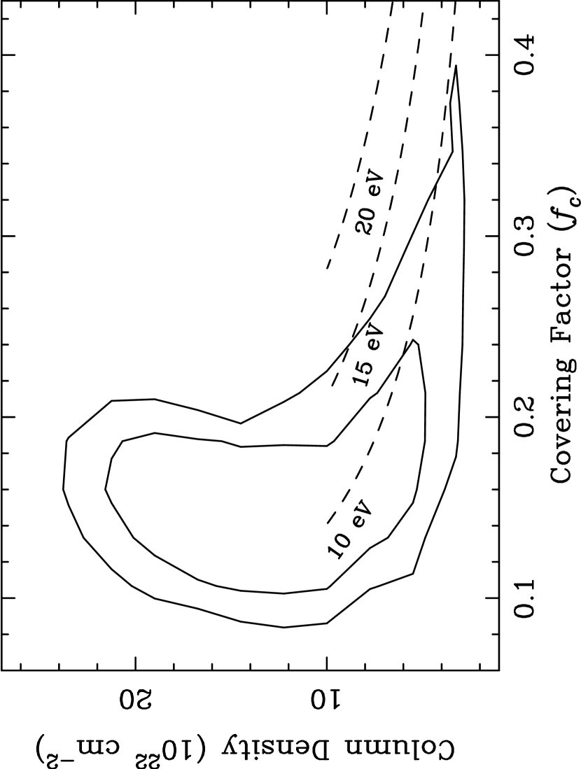
Figure 10.— Confidence contours in the column density and covering fraction for the partial covering powerlaw model described in §5.3.3. As described in §5.3.3, the absorber is expected to produce an Fe K${\rm\alpha}\,$emission line. Overlaid on the contours are lines of constant Fe K${\rm\alpha}\,$equivalent width (10,15, and 20 eV) as a function of $N_{\rm H,2}$ and $f_{c}$ as prescribed by equation (1).

Figure 11.— Confidence contours for the Gaussian fit to the residual Fe K${\rm\alpha}\,$emission line from the partial covering model (with the soft Gaussian included) described in §5.3.3. The equivalent width is defined to be the line flux divided by the specific continuum flux at energy E.

References

- Anders & Grevesse (1989) Anders, E. & Grevesse, N. 1989, Geochim. Cosmochim. Acta, 53, 197
- Anders & Ebihara (1982) Anders, E. & Ebihara, M. 1982, Geochim. Cosmochim. Acta, 46, 2363
- Arnaud (1996) Arnaud, K. A. 1996, ASP Conf. Ser. 101: Astronomical Data Analysis Software and Systems V, 5, 17
- Ballantyne et al. (2004) Ballantyne, D. R., Fabian, A. C., & Iwasawa, K. 2004, MNRAS, 354, 839
- Ballantyne et al. (2001) Ballantyne, D. R., Iwasawa, K., & Fabian, A. C. 2001, MNRAS, 323, 506
- Ballantyne et al. (2002) Ballantyne, D. R., Ross, R. R., & Fabian, A. C. 2002, MNRAS, 332, L45
- Bianchi et al. (2004) Bianchi, S., Matt, G., Balestra, I., Guainazzi, M., & Perola, G.C. 2004, A&A, 422, 65
- Beloborodov (1999) Beloborodov, A. M. 1999, ApJ, 510, L123
- Chen & Halpern (1989) Chen, K., & Halpern, J.P. 1989, ApJ, 339, 742
- Done et al. (1992) Done, C., Mulchaey, J. S., Mushotzky, R. F., & Arnaud, K. A. 1992, ApJ, 395, 275
- Elvis et al. (1989) Elvis, M., Lockman, F. J., & Wilkes, B. J., 1989, AJ, 97, 777
- Eracleous & Halpern (1998) Eracleous, M. & Halpern, J. P. 1998, American Institute of Physics Conference Series, 431, 261
- Eracleous et al. (1996) Eracleous, M., Halpern, J. P., & Livio, M. 1996, ApJ, 459, 89
- Eracleous et al. (2000) Eracleous, M., Sambruna, R., & Mushotzky, R. F. 2000, ApJ, 537, 654
- Dewangan et al. (2003) Dewangan, G. C., Griffiths, R. E., & Schurch, N. J. 2003, ApJ, 592, 52
- Fabian et al. (1989) Fabian, A. C., Rees, M. J., Stella, L., & White, N. E. 1989, MNRAS, 238, 729
- Fabian et al. (1995) Fabian, A. C., Nandra, K., Reynolds, C. S., Brandt, W. N., Otani, C., Tanaka, Y., Inoue, H., & Iwasawa, K. 1995, MNRAS, 277, L11
- Fanaroff & Riley (1974) Fanaroff, B. L. & Riley, J. M. 1974, MNRAS, 167, 31P
- Gavazzi & Perola (1978) Gavazzi, G. & Perola, G. C. 1978, A&A, 66, 407
- Gelbord (2003) Gelbord, J. M. 2003, Ph.D. Thesis, (available at http://space.mit.edu/ jonathan/papers/thesis/)
- George & Fabian (1991) George, I. M. & Fabian, A. C. 1991, MNRAS, 249, 352
- Ghisellini et al. (1994) Ghisellini, G., Haardt, F., & Matt, G. 1994, MNRAS, 267, 743
- Gliozzi et al. (2003) Gliozzi, M., Sambruna, R., & Eracleous, M. 2003, ApJ, 584, 176
- Gondek et al. (1996) Gondek, D., Zdziarski, A. A., Johnson, W. N., George, I. M., McNaron-Brown, K., Magdziarz, P., Smith, D., & Gruber, D. E. 1996, MNRAS, 282, 646
- Grandi et al. (1997) Grandi, P., Sambruna, R. M., Maraschi, L., Matt, G., Urry, C. M., & Mushotzky, R. F. 1997, ApJ, 487, 636
- Grandi et al. (2001a) Grandi, P., Maraschi, L., Urry, C. M., & Matt, G. 2001, ApJ, 556, 35
- Grandi (2001b) Grandi, P. 2001, Memorie della Societa Astronomica Italiana, 72, 91
- Halpern (1982) Halpern, J. P. 1982, Ph.D. Thesis, Harvard
- Iwasawa et al. (1996) Iwasawa, K., et al. 1996, MNRAS, 282, 1038
- Kirsch et al. (2004) Kirsch, M. G. F. et al. 2004, Proc. SPIE, 5488, in press (astro-ph/0407257)
- Lee et al. (1999) Lee, J. C., Fabian, A. C., Brandt, W. N., Reynolds, C. S., & Iwasawa, K. 1999, MNRAS, 310, 973
- Lightman & White (1988) Lightman, A. P. & White, T. R. 1988, ApJ, 335, 57
- Linfield & Perley (1984) Linfield, R. & Perley, R. 1984, ApJ, 279, 60