SPECTROSCOPIC-LIKE TEMPERATURE OF CLUSTERS OF GALAXIES AND COSMOLOGICAL IMPLICATIONS

The thermal properties of hydrodynamical simulations of galaxy clusters are usually compared to observations by relying on the emission-weighted temperature $T_{\rm ew}$, instead of on the spectroscopic X-ray temperature $T_{\rm spec}$, which is obtained by actual observational data. Here we show that, if the intra-cluster medium is thermally complex, $T_{\rm ew}$ fails at reproducing $T_{\rm spec}$. We propose a new formula, the spectroscopic-like temperature, $T_{\rm sl}$, which approximates $T_{\rm spec}$ better than a few per cent. By analyzing a set of hydrodynamical simulations of galaxy clusters, we also find that $T_{\rm sl}$ is lower than $T_{\rm ew}$ by 20–30 per cent. As a consequence, the normalization of the $M$–$T_{\rm sl}$ relation from the simulations is larger than the observed one by about 50 per cent. If masses in simulated clusters are estimated by following the same assumptions of hydrostatic equilibrium and $\beta$–model gas density profile, as often done for observed clusters, then the $M$–$T$ relation decreases by about 40 per cent, and significantly reduces its scatter. Based on this result, we conclude that using the observed $M$–$T$ relation to infer the amplitude of the power spectrum from the X–ray temperature function could bias low $\sigma_{8}$ by 10-20 per cent. This may alleviate the tension between the value of $\sigma_{8}$ inferred from the cluster number density and those from cosmic microwave background and large scale structure.

1 Introduction

Clusters of galaxies represent a powerful tool for investigating cosmological parameters like the normalization of the primordial power spectrum, usually expressed in terms of $\sigma_{8}$ (e.g. Rosati et al. 2002). The fundamental quantity entering theoretical models is the cluster mass, $M$, but its high-precision measurement is still precluded by the presence of different systematic effects.

One way to derive $M$ comes indirectly from the X-ray temperature $T$, which is related to the cluster mass. In fact simple theoretical arguments suggest for virialized systems the existence a $M$–$T$ scaling law. The $M$–$T$ relation is one of the key ingredients in the recipes to extract cosmological parameters from the cluster temperature function (XTF) which also requires a proper comparison between simulated and observed data. Although simple in principle, this comparison is not always trivial. Projection effects and/or instrumental factors introduce systematic biases that complicate the correct interpretation of the data. To overcome this difficulty we built the X-ray MAp Simulator (X-MAS, Gardini et al. 2004), a software package devoted to simulate X-ray observations of galaxy clusters obtained from hydro-N-body simulations. Using X-MAS we showed that, if the cluster is highly thermally inhomogeneous, then the projected spectroscopic temperature $T_{\rm spec}$, obtained from the fit of the observed spectrum, is significantly lower than the emission-weighted temperature $T_{\rm ew}$, which may be directly inferred from the simulations by weighting each particle temperature by its emission measure. Depending on the thermal complexity of the clusters, this discrepancy may affect the normalization of the $M$–$T$ relation and, consequently, the amplitude of the power spectrum $\sigma_{8}$ derived from the XTF.

In Mazzotta et al. (2004) we studied in detail the problem of performing a proper comparison between temperatures obtained from X-ray observations and simulations. We found that although in principle this comparison requires the actual simulation of the spectral properties of the clusters, when the cluster temperature is higher than $T>2-3$ keV, it is possible to define a new “spectroscopic-like temperature” function $T_{\rm sl}$, that approximates $T_{\rm spec}$ to better that few percent. In this paper we highlight the main aspects connected with the derivation of $T_{\rm sl}$  and, thanks to a set of hydrodynamical simulations of galaxy clusters, we discuss the implications for the $M$–$T$ relation and for the determination of $\sigma_{8}$.

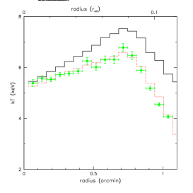
Figure 1: Temperature profiles of the simulated galaxy cluster. Filled circles indicate the spectroscopic temperature profile from Gardini et al. (2003); error bars are at $68$ per cent confidence level for one interesting parameter. Solid and dotted histogram refer to the mean emission-weighted and spectroscopic-like temperature profiles directly derived from the simulation for the same annulus regions.

2 Spectroscopic-like temperature

From a purely analytic point of view the spectroscopic temperature $T_{\rm spec}$  is not a well defined quantity. In fact, it results from the fit of a single-temperature thermal model to a multi-temperature source spectrum; however, since the former cannot accurately reproduce the spectral properties of the latter, it follows that $T_{\rm spec}$  cannot be unequivocally identified. Despite of this, as observed spectra are affected by a number of factors that distort and confuse some of their properties, in some circumstances multi-temperature thermal source spectra may appear statistically indistinguishable from single-temperature ones. In Mazzotta et al. (2004) we discuss this aspect by focusing our attention on observations of clusters of galaxies made using the CCD detectors of Chandra  and XMM-Newton. From this study we find two very important results that we summarize as:
i) given a multi-temperature source spectrum, if the lowest dominant temperature component has $T_{1}>2-3$ keV, then a fit made with a single-temperature thermal model is statistically acceptable regardless of the actual spread of the temperature distribution of the source;
ii) the emission-weighted temperature $T_{\rm ew}$  does not properly estimate the spectroscopic temperature $T_{\rm spec}$  as it tends to overestimate it. The larger the spread in temperature of the thermal components of the observed spectra, the larger the discrepancy.

To partially solve this problem we propose to use the spectroscopic-like temperature function $T_{\rm sl}$ instead of $T_{\rm ew}$. The idea behind the analytic derivation of $T_{\rm sl}$  is quite simple and is itemized below.

• Given a multi-temperature source spectrum we are interested in identifying the temperature $T_{\rm sl}$ whose spectrum is closest to the observed one. If for simplicity we consider a source spectrum composed by two thermal models with densities $n_{1}$, $n_{2}$ and temperatures $T_{1}$, $T_{2}$ respectively, requiring matching spectra means that:

  $$\begin{array}[]{l}n_{1}^{2}\zeta(Z,T_{1})\frac{1}{\sqrt{T}_{1}}\exp(-\frac{E}{kT_{1}})+n_{2}^{2}\zeta(Z,T_{2},)\frac{1}{\sqrt{T}_{2}}\exp(-\frac{E}{kT_{2}})\\ \approx A\zeta(Z,T_{sl})\frac{1}{\sqrt{T}_{sl}}\exp(-\frac{E}{kT_{sl}}),\\ \end{array}$$ (1)

  where $A$ is an arbitrary normalization constant and $\zeta(Z,T)$ is a parameterization function accounting for the total Gaunt factor and partly for the line emission. We approximate $\zeta(Z,T,E)\propto(T/{\rm keV})^{\alpha}$.

• Supported by the fact that both Chandra  and XMM-Newton  are more sensitive to the soft region of the X-ray spectrum, we can expand the previous equation in Taylor series to the first order of $E/kT$ and obtain:

  $$T_{\rm sl}=\frac{\sum_{i}n_{i}^{2}T_{i}^{\alpha}/T_{i}^{1/2}}{\sum_{i}n_{i}^{2}T_{i}^{\alpha}/T_{1}^{3/2}},$$ (2)

  where we generalized to an arbitrary number of thermal components for the source spectrum.

• The power index $\alpha$ needs to be calibrated to the specific detector. This can be done by simulating a set of two-temperature source spectra and minimizing the value of the mean percentile variation of $T_{\rm sl}$ with respect to $T_{\rm spec}$. In Mazzotta et al. (2004) we show that $\alpha=3/4$ represent a good choice for each CCD detector of Chandra  and XMM-Newton.

It is important to say that we tested $T_{\rm sl}$  against $T_{\rm spec}$, and $T_{\rm ew}$  by using the hydro-N-body simulation of a thermally complex (major merger) cluster of galaxies and by applying X-MAS. We compared the projected temperature maps and profiles derived by using different temperature definitions. We find that $T_{\rm sl}$  approximate $T_{\rm spec}$  to better than few percent, while $T_{\rm ew}$  may overestimate $T_{\rm spec}$  by factors as large as 2 (see Mazzotta et al. 2004 for details). Just as an example in Fig. 1 we show the azimuthally averaged temperature profiles of this cluster as obtained by adopting the three different estimators. It is worth noticing that while $T_{\rm sl}$  is consistent within the errors with $T_{\rm spec}$, $T_{\rm ew}$  is always higher.

3 Cosmological implications

In this section we discuss the consequences of the discrepancy between $T_{\rm spec}$  and $T_{\rm ew}$  for the $M$–$T$ relation and for the estimate of $\sigma_{8}$ from the XTF. To do that we present the analysis of a sample of hydrodynamical simulations of galaxy clusters for which we use the temperature function $T_{\rm sl}$  defined in the previous paragraph. The results presented here are extracted from Rasia et al. (2005) to which we refer for more details.

We created the sample of simulated galaxy clusters by merging two different sets:

• Set#1: 95 temperature-selected clusters (with $T_{\rm ew}>2$ keV), extracted from the large-scale cosmological hydro-N-body simulation of a “concordance” $\Lambda$CDM model ($\Omega_{0m}=0.3$, $\Omega_{0\Lambda}=0.7$, $\Omega_{0\rm b}=0.019\,h^{-2}$, $h=0.7$, $\sigma_{8}=0.8$), presented in Borgani et al. (2004, B04)

• to account for the high temperature ($T>7$ keV) clusters not present in Set#1 because of the limited box size of the previous simulation, we added a Set#2 composed by clusters having $M_{\rm vir}>10^{15}h^{-1}M_{\odot}$ belonging to a different set of high-resolution hydro-N-body simulations (Dolag et al. 2005 in preparation).

Besides gravity and hydrodynamics, both simulations includes the treatment of radiative cooling, the effect of a uniform time–dependent UV background, a sub–resolution model for star formation from a multiphase interstellar medium, as well as galactic winds powered by SN explosions (Springel & Hernquist 2003).

For each cluster in our sample we calculate both $T_{\rm ew}$ and $T_{\rm sl}$. In Fig. 3 we plot the values of $T_{\rm sl}$ versus $T_{\rm ew}$. The distribution of the points in Fig. 3 suggests that the two estimators can be roughly related by a linear relation. By applying a $\chi^{2}$ fit, we find $T_{\rm sl}=(0.70\pm 0.01)T_{\rm ew}+(0.29\pm 0.05)$, shown as dotted line in Fig. 3.

The existence of a systematic trend between the two different estimates of the cluster temperature has interesting consequences on the $M$–$T$ scaling relation. Using Set$\#1$, Borgani et al. (2004) showed that the normalization ($M_{0}$) of the simulated $M$-$T_{\rm ew}$ relation is 20% higher than the observed one. Since $T_{\rm ew}$ tends to overestimate $T_{\rm sl}$ by a fair amount, we expect the actual $M$-$T_{\rm sl}$ relation from simulations to be even more discrepant with respect to observations. In fact, we find that $M_{0}$ is higher than the observed one by about 50 per cent. However, in order to compare the $M$-$T$ obtained in observations and simulations, it is also necessary to derive the simulated clusters mass under the same assumption of the X-ray analysis, i.e. by applying the condition of hydrostatic equilibrium to a spherical gas distribution described by a $\beta$–model (Cavaliere & Fusco–Femiano 1976), with the equation of state having a polytropic form. In this way, the total self–gravitating mass within the radius $r$ is given by (Finoguenov et al. 2001; Ettori et al. 2002),

$$M(<r)\,=\,1.11\times 10^{14}\beta_{\rm fit}\gamma{T(r)\over{\rm keV}}{r\over h^{-1}Mpc}{x^{2}\over 1+x^{2}}\,h^{-1}M_{\odot}.$$ (3)

Here $T(r)$ is the temperature at $r$, $\beta_{\rm fit}$ is the fitted slope of the gas density profile, $x\equiv r/r_{c}$ is the radial coordinate in units of the core radius $r_{c}$, and $\gamma$ is the effective polytropic index obtained from temperature and gas profiles. Fitting the simulation results gives $\log(M_{0}/h^{-1}M_{\odot})=13.41\pm 0.13$ when fixing $\alpha=1.5$.

As already mentioned, the $M$–$T$ relation is one of the key ingredients in the recipes to extract cosmological parameters from the cluster XTF: under the reasonable assumption that the scaling relations do not significantly change with $\sigma_{8}$, a larger $M_{0}$ implies a larger mass for a fixed temperature and, therefore, a higher normalization of the power spectrum (e.g., Borgani et al. 2001; Seljak 2002; Pierpaoli et al. 2003; Henry 2004). Huterer & White (2002) suggested an approximation for the scaling of $\sigma_{8}$ with $M_{0}$, involving the matter density parameter: $\Omega_{0m}^{0.6}\sigma_{8}\propto M_{0}^{0.53}$. Based on this relation and on the fact that a number of analyses of hydrodynamical simulations (e.g., Muanwong et al. 2002; B04; Rasia et al. 2004; Kay et al. 2004) have shown that Eq.3 underestimates the actual cluster mass by about 20%, we expect that the value of $\sigma_{8}$ is underestimated by a similar amount, i.e. about 20%.

In Fig.3 we show the effect on the XTF of using $T_{\rm sl}$, instead of $T_{\rm ew}$. We compare here the cumulative temperature function $N(>T)$ from the simulation (Set#1 only) to the data by Ikebe et al. (2002). The squared points represent the emission-weighted temperature; being $T_{\rm ew}$ in good agreement with the data, one could argue that the $\sigma_{8}$ used in the simulation well represents the observed universe. This would imply $\sigma_{8}=0.8$. However, as already shown, the emission-weighted temperature is typically an underestimate of the observed temperature, while the spectroscopic-like temperature better takes into account the observational procedure of temperature measurement. The comparison between $T_{\rm sl}$ and data shows that $\sigma_{8}=0.8$ is excluded at 3$\sigma$ level, while favoring a larger power spectrum normalization, at least for the ICM physics included in our simulation. Computing the mass function by Sheth & Tormen (1999) for our cosmology at the mass corresponding to a 2 keV cluster, we find that $\sigma_{8}$ needs to be increased to about 0.9 to increase the number density of clusters above this mass limit by the required 50–60 per cent.

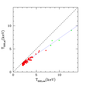
Figure 2: The comparison between $T_{\rm ew}$ and $T_{\rm sl}$. Circles and triangles refer to objects from Set#1 and Set#2, respectively. The dotted line is the best fit, while the dashed line corresponds to $T_{\rm sl}=T_{\rm ew}$.

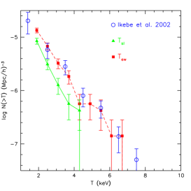
Figure 3: The cumulative temperature function $N(>T)$, from Set#1. Filled squares and dashed line refer to the results for $T_{\rm ew}$, while filled triangles and solid line represent $T_{\rm sl}$. Error bars correspond to Poissonian uncertainties. For reference, open circles show the local temperature function measured by Ikebe et al. (2002).

4 Conclusions

In this section we simply summarize the main results presented in this paper.

1. The projected spectroscopic temperature $T_{\rm spec}$  of thermally complex clusters obtained from X-ray observations is always lower than the emission-weighed temperature $T_{\rm ew}$, which is instead widely used in the analysis of numerical simulations. We show that this temperature bias is mainly related to the fact that the emission-weighted temperature does not reflect the actual spectral properties of the observed source.

2. A proper comparison between simulations and observations needs the actual simulations of spectral properties of the simulated clusters. Nevertheless, if the cluster temperatures is $>2-3$ keV it is possible to define a temperature function, that we call spectroscopic-like temperature $T_{\rm sl}$, which approximate $T_{\rm spec}$  to better than few per cent.

3. By analyzing a sample of hydrodynamical simulations of galaxy clusters, we find that $T_{\rm sl}$ (and, thus $T_{\rm spec}$) is lower than $T_{\rm ew}$ by 20–30 per cent. We obtain a linear fit approximating the relation between the two different temperature estimators. As previous studies made using $T_{\rm ew}$ show that the discrepancy in the $M$–$T$ relation between simulations and observations is about 20 per cent, it is clear that the use of $T_{\rm sl}$ increases this discrepancy to $\sim 50$ per cent. Nevertheless, if we assume hydrostatic equilibrium for the gas density distribution described by a $\beta$–model with a polytropic equation of state, we know that masses are underestimated on average by $\sim 40$ per cent. Although this goes in the direction of substantially reducing the discrepancy with observational data, this is not sufficient to cancel it.

4. The bias in the $M$–$T$ relation propagates into a bias in $\sigma_{8}$, from the XTF. If such a bias is as large as that found in our simulations, the values of $\sigma_{8}$ obtained by combining the local XTF and the observed $M$–$T$ relation are underestimated by about 15 per cent.

5. The XTF from the simulation is significantly lower when using $T_{\rm sl}$ instead of $T_{\rm ew}$. A comparison with the observed XTF indicates that for the “concordance” $\Lambda$CDM model $\sigma_{8}$ needs to be increased from $\simeq 0.8$ to $\simeq 0.9$.

To conclude, the results of this study go in the direction of alleviating a possible tension between the power–spectrum normalization obtained from the number density of galaxy clusters and that arising from the first–year WMAP CMB anisotropies (e.g. Bennett et al. 2003) and SDSS galaxy power spectrum (e.g. Tegmark et al. 2004).

References

References

- [1] Bennett, C.L., et al. 2003, ApJS, 148, 1
- [2] Borgani, S., et al. 2001, ApJ, 561, 13
- [3] Borgani, S., et al. 2004, MNRAS, 348, 1078 (B04)
- [4] Cavaliere, A., & Fusco–Femiano, R. 1976, A&A, 49, 137
- [5] Ettori, S., De Grandi, S., & Molendi, S. 2002, A&A, 391, 841
- [6] Finoguenov, A., Reiprich, T.H., & Böhringer, H. 2001, A&A, 369, 479
- [7] Gardini, A., Rasia, E., Mazzotta, P., Tormen, G., De Grandi, S., & Moscardini, L. 2004, MNRAS, 351, 505
- [8] Henry, J.P. 2004, ApJ, 609, 603
- [9] Huterer, D., & White, M. 2002, ApJ, 578, L95
- [10] Ikebe, Y., et al., 2002, A&A, 383, 773
- [11] Kay, S.T., Thomas, P.A., Jenkins, A., & Pearce, F.R. 2004, MNRAS, tmp,504
- [12] Mazzotta, P., Rasia, E., Moscardini, L., & Tormen, G. 2004, MNRAS, 354, 10
- [13] Muanwong, O., Thomas, P.A., Kay, S.T., & Pearce, F.R. 2002, MNRAS, 336, 527
- [14] Pierpaoli, E., Borgani, S., Scott, D., & White, M. 2003, MNRAS, 342, 163
- [15] Rasia, E., Tormen, G., & Moscardini, L. 2004, MNRAS, 351, 237
- [16] Rasia, E., Mazzotta, P., Borgani, S., Moscardini, L., Dolag, K., Tormen, G., Diaferio, A., & Murante, G. 2005, ApJ, 618, L1
- [17] Rosati, P., Borgani, S., & Norman, C. 2002, ARA&A, 40, 539
- [18] Seljak, U. 2002, MNRAS, 337, 769
- [19] Sheth, R.K., & Tormen, G. 1999, MNRAS, 308, 119
- [20] Springel, V., & Hernquist, L. 2003, MNRAS, 339, 289
- [21] Tegmark, M., et al. 2004, Phys. Rev. D, 69, 103501