Constraints on the star formation history of the Large Magellanic Cloud

We present the analysis of deep colour-magnitude diagrams (CMDs) of 6 stellar fields in the LMC. The data were obtained using HST/WFPC2 in the F814W ($\sim$ I) and F555W ($\sim$ V) filters, reaching $\mathrm{V_{555}\sim 26.5}$. We discuss and apply a method of correcting CMDs for photometric incompleteness. A method to generate artificial CMDs based on a model star formation history is also developed. This method incorporates photometric error effects, unresolved binaries, reddening and allows use of different forms of the initial mass function and of the SFH itself. We use the Partial Models Method, as presented by Gallart and others, for CMD modelling, and include control experiments to prove its validity in a search for constraints on the Large Magellanic Cloud star formation history in different regions. Reliable star formation histories for each field are recovered by this method. In all fields, a gap in star formation with $\tau\sim$ 700 Myrs is observed. Field-to-field variations have also been observed. The two fields near the LMC bar present some significant star forming events, having formed both young ($\tau$ $\;\buildrel<\over{\sim}\;$$1\leavevmode\nobreak\ Gyr$) and old ($\tau$ $\;\buildrel>\over{\sim}\;$$10\leavevmode\nobreak\ Gyr$) stars, with a clear gap from $3-6$ Gyrs. Two other fields display quite similar SFHs, with increased star formation having taken place at $\tau\simeq 2-3Gyrs$ and $6$ $\;\buildrel<\over{\sim}\;$$\tau$ $\;\buildrel<\over{\sim}\;$$10Gyrs$. The remaining two fields present star formation histories closer to uniform, with no clear event of enhanced star formation.

1 Introduction

The study of the star formation history (SFH) in near galaxies can contribute to our understanding of the evolution of these objects, the mechanisms involved in the star formation bursts, their associated time scales, and the initial stellar mass function (IMF). Star formation time scales and IMFs are particularly important, being used as input for population synthesis models which try to interpret integrated light from distant galaxies to obtain information about their component stars. Moreover, by matching SFH to dynamical models, it is possible to investigate the influence of gravitational interactions on star formation.

The Large Magellanic Cloud (LMC) is a satellite of the Galaxy, being at the same time quite distinct from it and yet near enough to it to allow a study of its structure, internal kinematics and stellar populations (Westerlund 1990). By its proximity and nature, the LMC provides an excellent laboratory for the study of the processes involved in star formation, such as interactions with neighboring galaxies (especially the Galaxy and the Small Magellanic Cloud (SMC)), the influence of bar dynamics and chemical enrichment (Gardiner et al. 1998).

The main advantage of LMC stellar population studies is the ability to build detailed colour-magnitude diagrams (CMDs) in various regions within it. Furthermore, the LMC supplies a unique chance to compare the inferred SFH through the study of field stars with the SFH found from studies of its cluster system. The reason is that the LMC presents a rich cluster population of largely varying ages. Cluster CMDs have the advantage of being composed of a single population, making their analysis much simpler. Studies using LMC clusters show that the majority of them are relatively young, with ages $\tau$ $\;\buildrel<\over{\sim}\;$4 Gyr, a small number has $\tau$ $\;\buildrel>\over{\sim}\;$10 Gyr and only one is of intermediate age ($\tau\sim$ 8 Gyr) (Mateo, Hodge & Schommer 1986). However, only a small fraction of LMC stars belong to clusters, rendering the field CMD analyses of more general interest and more representative of the global SFH.

Ground-based CMD studies have favoured a predominance of young or intermediate-age populations in the LMC. Bertelli et al. (1992), for example, have analyzed CMDs in a few LMC outer regions and modelled them with a single-burst SFH with $\tau\sim$ 2 – 4 Gyr, with a factor of $\sim 10$ increase relative to the average quiescent star formation, the exact burst age being dependent on the details of stellar evolutionary theories available then. The same group also found some evidence for field-to-field variations in SFH (Vallenari et al. 1996).

Earlier ground-based work did not reach deep enough magnitudes to directly access the main sequence turn-offs of stellar populations with ages $\tau$ $\;\buildrel>\over{\sim}\;$6 Gyr. This became possible only with the use of the Hubble Space Telescope (HST), whose images were free of atmospheric turbulence and, therefore, much sharper and deeper. Gallagher et al. (1996), based on a single HST Wide Field and Planetary Camera 2 (WFPC2) field, suggested a roughly constant star formation rate (SFR) in the past few Gyr, except for a small period of enhanced star formation about 2 Gyr ago. Holtzman et al. (1997) analyzed the luminosity function of the same HST field, located some 4$\degr$ from LMC bar, and favoured a constant SFR for 10 Gyr in the LMC, followed by an increase factor of 3 in the last 2 Gyr, yielding roughly the same number of stars younger and older than 4 Gyr. They also identified an intermediate-age turn-off in their field CMD. Elson, Gilmore & Santiago (1997) studied an HST field closer to the LMC bar and identified two main populations, with ages $\tau\,\sim$ 1 – 2 Gyr and $\tau\,\sim$ 2 – 4 Gyr, the exact ages depending on their metallicity. Geha et al. (1998) have studied 3 HST fields in the outer region of the LMC and also suggested a model with roughly equal numbers of stars younger and older than $\tau=$ 4 Gyr. Studying fields inside the LMC bar, Olsen (1999) suggested that the star formation has been more continuous, possibly extending back for a longer period and taking place at a roughly constant SFR as compared to the outer fields. This differs from the conclusions of Elson, Gilmore & Santiago (1997). Holtzman et al. (1999) have not found obvious evidence for bursts of star formation and concluded that the field SFH differs from that based on the LMC cluster age distribution.

In this paper, we describe the CMD modelling of 6 deep HST fields located in different directions along the LMC, all of them within $6^{\circ}$ of the LMC centre. Our main goal is to recover information about the SFH of the LMC field population, the age-metallicity relation $Z(\tau)$ and IMF. Our samples have been combined with those of a previous paper (Castro et al. 2001) and make up an extended, deep and homogeneous photometric dataset. The paper is outlined as follows: in Sect. 2 we describe the HST/WFPC2 data, the stellar samples derived from them, and the photometry, including methods of accounting for sample incompleteness. The combined sample is presented in Sect. 3; in Sect. 4 we present the CMD modelling algorithm, which is essentially the Partial Models Method (PMM) by Gallart et al. (1999), Aparicio et al. (2001) and Carrera et al. (2002), and discuss the statistical tools used in our model vs. data comparisons; finally, in Sect. 5 we present the results, which are discussed in Sect. 6.

2 Observations and data reduction

We use data obtained with the Wide Field and Planetary Camera 2 (WFPC2) on board HST for 6 fields near the rich LMC clusters NGC1805, NGC1818, NGC1831, NGC1868, NGC2209 and Hodge 11. These data are part of the GO7307 project entitled “Formation and Evolution of Rich Star Clusters in the LMC” (Beaulieu et al. 1999; Kerber et al. 2002; de Grijs et al. 2002). For each field, a set of at least 2 exposures were obtained using each of the F814W (I) and F555W (V) filters. The main properties of the fields (hereafter identified by their nearby rich LMC cluster) are given in Table 1: columns 2 and 3 list their equatorial coordinates (J2000), followed by their angular distance from the LMC optical centre, total I and V exposure times and the number of individual exposures taken with each filter.

All exposures were put through the standard HST pipeline procedure that corrects them for several instrumental effects, such as bias and dark currents and flat-fielding (Holtzman et al. 1995a). The exposures taken in each field/filter configuration were then combined using the IRAF task CRREJ, in order to increase the signal to noise ratio and remove cosmic rays. The final combined image at each configuration was then used for sample selection and photometry.

Table 1: Basic characteristics of the our HST/WFPC2 fields. The columns show the field name, equatorial coordinates (J2000), angular distance with respect to the LMC centre, total exposure times and the number of exposures in I and V. Note that the identification of each field is related to the rich LMC cluster parallel to which it was observed.

Field	$\alpha$ (h m s)	$\delta$ ($\deg\leavevmode\nobreak\ \arcmin\leavevmode\nobreak\ \arcsec$)	Ang.	$t_{I}$	$t_{V}$	$N_{I}$	$N_{V}$
	$(2000)$	$(2000)$	Dist. ($\degr$)	$(s)$	$(s)$
NGC1805	5 01 42	-65 59 58	4.28	2200	2200	2	2
NGC1818	5 05 00	-66 25 13	3.75	4800	7200	4	6
NGC1831	5 05 21	-64 49 50	1.51	2200	2200	2	2
NGC1868	5 13 48	-63 52 10	5.96	2200	2200	2	2
NGC2209	6 07 39	-73 46 07	5.28	4800	7200	4	6
Hodge 11	6 15 07	-69 49 08	4.44	4800	7200	4	6

2.1 Sample selection

The IRAF DAOPHOT package was used to detect and classify sources automatically in each combined image, i. e. the sample selection was carried out independently in each photometric band. Star candidates were detected using DAOFIND, with a peak intensity threshold for detection set to $5\,\sigma$, where $\sigma$ corresponds to the rms fluctuation in the sky counts, determined individually for each combined image.

Figure 1: Observed colour-magnitude diagram of the field near NGC1818.

A preliminary aperture ($radius=2\arcsec$) photometry was carried out by running the task PHOT on all objects output by DAOFIND. Star/galaxy separation required modelling point sources by fitting the profiles of bright, isolated and non-saturated stars to a Moffat function ($\beta=1.5$). We used the IRAF task PSF for that purpose. This PSF model was then fitted to all objects found by DAOFIND with the ALLSTAR task.

The output parameters given by ALLSTAR ($\chi^{2}$, sharpness, magnitude uncertainties $\mathrm{\delta I}$ and $\mathrm{\delta V}$) are useful to separate a purely stellar sample from the remaining detected sources, like distant galaxies. Stellar sources present small $\mathrm{\delta I}$ and $\mathrm{\delta V}$ values. Thus we threw away objects with $\mathrm{\delta I}$ or $\mathrm{\delta V}$ greater than a constant value, typically $\sim$ 0.15 mag. These cut off values were chosen separately for each field/filter, based on visual inspection of the more conspicuous stellar and non-stellar cases. This stellar/non-stellar classification was checked by visual inspection of the stellar sample selected and iterated when necessary, until a “clean” stellar sample resulted. The final stellar sample in each field, and which was used in the subsequent CMD analysis and modelling, was the merging result of stars selected in both bands, i. e., with small values of $\mathrm{\delta I}$ and $\mathrm{\delta V}$ measured by ALLSTAR.

Figure 1 shows the final observed CMD of the field near the cluster NGC1818. One can see a main sequence (MS) that stretches down to $\mathrm{V_{555}\sim V=26.5\,}$. The saturation limit, also found using the ALLSTAR $\mathrm{\delta I}$ and $\mathrm{\delta V}$ parameters (saturated stars display large magnitude uncertainties from PSF fitting), was found to be about $\mathrm{V_{555}=18.5}$ for this field. The red giant branch (RGB) is visible as well, along with a turn-off around $\mathrm{V_{555}\simeq 22.5\,}$ This latter corresponds to an old population ($\tau$ $\;\buildrel>\over{\sim}\;$10 Gyr, as shown in Castro et al. 2001). The red giant clump (RC), found in intermediate-age populations, is also visible at $\mathrm{V_{555}\sim 19}$ and $\mathrm{V_{555}-I_{814}\sim 0.9\,}$. The faint red stars at the right of the CMD are likely low-luminosity M dwarfs in the Galaxy. The other 5 deep LMC fields in our sample display the same general features described above.

The data suffer from an important effect: sample incompleteness. Our CMD modelling algorithm (presented in §4) therefore needs to incorporate such an effect in order to place models and data on equal footing. Quantifying photometric uncertainties and applying them to the model CMDs is extremely important as well, as they are responsible for most of the observed CMD spread. These data corrections are the subject of the next subsections.

2.2 Photometric uncertainties

There are two approaches to quantify photometric uncertainties: an empirical approach, through the comparison of independent magnitude measurements of the same object, or a semi-empirical approach, in which the photometric uncertainties follow from the measured signal and an adopted model for the associated noise, such as that used by the IRAF task PHOT. In the empirical approach, one needs two or more images of identical characteristics, such as total exposure time, detector noise, etc. We unfortunately do not have two identical combined images for each field and filter.

We tried to use the independent magnitude measurements taken from individual exposures of each filter/field configuration in order to empirically estimate the photometric uncertainties in the combined images. However, the photometric error measured in a single exposure tends to be greater than that of the combined image, due to the smaller signal to noise ratio. Assuming Poissonic statistics of photon counts, overlooking detector noise and assuming $N$ individual exposures of the same exposure time, the scaled magnitude uncertainty of the combined image should be:

$$\delta m\propto\left(\frac{1}{\sqrt{N}}\right)$$ (1)

However, we failed to confirm the scaling in magnitude uncertainties given above, which suggests that the assumptions that lead to eq. 1 are over-simplistic. Therefore, we decided to rely on the model uncertainty from the IRAF PHOT task. These uncertainties take detector (readout) noise and background (sky) noise into account as well. The spread of stars in the CMD depends on the photometric uncertainties of both bands. This means that the expected spread in colour $\mathrm{\sigma_{colour}}$ is given by

$$\mathrm{\sigma_{colour}^{2}=\sigma_{I}^{2}+\sigma_{V}^{2}}$$ (2)

2.3 Sample completeness

In any image, bright stars, which are not the majority, are easily detected. The faint ones are often not detected. Photometric completeness is defined as the percentage of the total number of stars that were successfully included in the sample by the detection and selection process. The knowledge of the completeness function is essential when the objective is to compare an observed CMD to model ones, with the goal of reconstructing an SFH. We thus carried out experiments to estimate the completeness function for each of our HST/WFPC2 fields. These experiments involved adding the same artificial stars, with a given magnitude and color, to the combined V and I images, and submitting these images, with real plus artificial stars, to the same detection and selection process as the real data. Thus, the extra stars were subjected to automatic detection with DAOFIND, to aperture photometry using PHOT, to PSF fitting and star/no-star separation using ALLSTAR and, finally, to the final matching of stellar lists in the I and V bands, as described in Sect. 2.1. Most previous works estimate completeness as a single variable function, such as C(V) or C(I), often overlooking variations in completeness along the color axis in a CMD. Others have computed single variable functions independently and have then taken their product in order to quantify completeness at any given CMD position (Mateo 1988). However, since the position within the field (and therefore the proximity to a bright star, for instance) is the same in both filters, the detection of a given star in the combined V image is not an event independent of detection of the same star in the combined I image. Thus, this latter approach invariably leads to an underestimate of completeness, the amplitude of the bias depending on issues such as field crowding, exposure times, etc. Our approach, by assigning a magnitude and colour to each artificial star and keeping the same CCD position for both filters, more effectively reproduces the true bi-variate completeness function. This resulting completeness function is then expressed as:

$$\mathrm{C(V-I,V)=\frac{recovered\>artificial\>stars\>in\>both\>V\>and\>I}{input\>artificial\>stars}}$$ (3)

Figure 2 shows an example of this bi-variate completeness function $\mathrm{C(V-I,V)}$. The completeness values are shown in percentage values (or $\mathrm{C(V-I,V)\times 100}$%). They are superposed on the CMD itself. It is possible to observe that, at faint magnitude levels, $\mathrm{C(V-I,V)}$ decreases with V magnitude, as expected. For V $\;\buildrel<\over{\sim}\;$26, however, the data seem to be largely complete. Moreover, $\mathrm{C(V-I,V)}$ is larger in the redder part of the low main sequence (for V $\;\buildrel>\over{\sim}\;$26). The latter effect may be easily understood as part of the selection process: faint stars in V, but bright in I (i.e., redder stars) have a larger probability to be selected than faint stars in both bands. This effect yields larger $\mathrm{C(V-I,V)}$ for redder V-I colours.

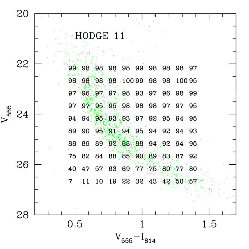
Figure 2: Observed colour-magnitude diagram of the field near Hodge 11 (dots). The number grid shows the $\mathrm{C(V-I,V)\times 100}$% completeness values for the same field, calculated according to the method described in §2.3.

The bi-variate $\mathrm{C(V-I,V)}$ function is used as a probability that a model star, generated according to the algorithm described in §4.1, is actually included in the sample. The details are left for that section. It is clear that the completeness function values suffer from some uncertainty. Therefore, our CMD analysis shown in §5 was restricted to CMD regions where completeness was close to unity (typically $\mathrm{V}\simeq 24.5-25.0$). Notice that the lower parts of the CMD are not crucial to the SFH reconstruction process, since the SFH is more strongly influenced by main-sequence turn-offs and the positions of evolved stars.

3 Combining different samples

In this work we have done the sample selection and photometry for 6 LMC fields. In Castro et al. (2001), 7 independent (or almost) LMC fields were studied. The data from both studies have a common origin, since they were observed with the same instrument and as part of the same project. All these fields are parallel HST/WFPC2 observations of a rich LMC cluster and therefore lie about 7.3 arcmin from this cluster. Therefore, our 6 fields can be paired with 6 of the fields studied by Castro et al. (2001). We thus decided to combine the stellar samples in each pair of fields in order to enhance the number of stars used in the CMD analysis.

In Figure 3, we compare the stellar luminosity function (LF) (upper panel) and the CMD (lower panel) of the two fields close to the rich LMC cluster NGC1831. The LF from our sample (dotted line in panel 3a) has been corrected for completeness, as described in §2.3. The LFs are very similar, the differences in star counts being in general consistent with random fluctuations ($\sqrt{N}$ bars are shown for the Castro et al. data). At the brightest magnitude bins ($V_{555}$ $\;\buildrel<\over{\sim}\;$$19.5$), the excess of stars from Castro et al. reflects their brighter saturation limit, caused by their shorter exposure time. At intermediate magnitudes, there may also exist a slight systematic excess of stars in the field studied by in Castro et al. (2001), suggesting that field-to-field variations in number counts are not entirely random. Even though the Castro et al. LF has not been corrected for sample incompleteness, this effect manifests itself only fainter than $V_{555}\sim 25$. The CMDs (panel 3b) from both samples match one another quite naturally, delineating the same loci. The RGBs are slightly displaced from each other (by $\Delta(V_{555}-I_{814})\sim 0.05$, in the sense of our data (open circles) being redder). This behavior is not uncommon in the other fields as well and probably result from PSF variations with time, which may in turn reflect optical variations, such as changes in telescope focus.

In order to place both samples in a common photometric system and thus avoid artificial spread in the combined sample CMD, we apply colour offsets to Castro et al. data. This was done by first defining a fiducial line for each separate sample, formed by the mean colour values at 0.25 magnitude bins along the MS. We then changed the $I_{814}$ magnitude values of Castro et al. (2001) so that the two fiducial lines would match each other. For the RGBs, we found a single colour difference and changed the $\mathrm{I_{814}}$ magnitudes from Castro et al. to bring them together. Typical corrections in colour were of $\sim 0.05$. Notice that this approach, besides being simple, yields a homogeneous photometric dataset, while preserving as much as possible of the original ($\mathrm{V_{555}}$, $\mathrm{V_{555}-I_{814}}$) CMD.

The final combined sample had to necessarily respect the differences in exposure time, sample selection and completeness corrections. Exposures times of Castro et al. 2001 data were smaller than ours. Consequently, their CMDs have more information on the bright part of the CMD, while our data have tend to better sample the faint part. Also, they applied no completeness correction to their sample. Therefore, we defined the following combination scheme:

1. For the bright CMD region (V $<19.5$) $\rightarrow$ only the Castro et al. stars were used;

2. For the faint CMD (V $>23.5$) $\rightarrow$ only our stars were included;

3. For the intermediate CMD ($19.5<$ V $<23.5$) $\rightarrow$ both samples were included;

The upper magnitude limit for our sample was meant to conservatively avoid any effect caused by saturation in our photometry. Likewise, the lower limit for Castro et al. stars is a conservative estimate of their completeness magnitude limits. The combination scheme adopted, of course, significantly alters the number counts along the observed CMD, since the effective solid angle covered by the sample is twice the size in the intermediate CMD regions than in the upper or lower ones. In Sect. 4 we describe how to incorporate this sampling effect in a model CMD. This is done simultaneously to the incorporation of completeness effects.

In two fields, the ones close to NGC1805 and NGC1831, some positional overlap exists between the fields studied here and those by Castro et al. (2001). Duplication of stars was prevented by using only our data in these overlapping regions. Positional matches between the two samples were found using the astrometry from the task METRIC available in the IRAF.STSDAS package. As the astrometric solutions for the overlapping fields were not unique, small positional offsets ($\simeq 0.5\arcsec$) were applied to the Castro et al. positions in order to make them comparable to ours.

Table 2 shows the results of our sample combination: column 2 lists the number of stars in our sample alone, whereas column 3 lists the number of stars in the composite sample. Both numbers correspond to stars brighter than the adopted completeness limit $\mathrm{V}\simeq 24.5-25.0$. The final stellar sample is markably greater than our original one, which translates into better statistics and more reliable CMD modelling.

Figure 3: (a) Luminosity functions of the field near NGC1831. Our sample is shown as a dotted line and that of Castro et al. (2001) as a solid line with Poissonic bars. (b) Observed colour-magnitude diagrams of our NGC1831 field (open circles) and that of Castro et al. (2001) (crosses).

Table 2: The result of combining the two photometric samples as discussed in §3. The columns show, respectively, field name, original number of stars in our sample and number of stars in the combined one.

Field		#stars		#stars
		our sample		composed sample
NGC1805		2576		3857
NGC1818		3566		5578
NGC1831		1040		1623
NGC1868		806		1395
NGC2209		1019		1483
Hodge 11		1420		2143

Figure 4: CMDs of the final combined samples for each of the fields, which are identified by the rich cluster close to which they lie.

Figure 4 shows the CMDs of the final combined sample for all 6 fields, which are again identified by the rich cluster close to which they lie. These may be directly compared to the CMDs shown by Castro et al. (2001) (figures 3 and 4). Apart from variations in magnitude limits, our final CMDs display the same features and have similar MS and RGB positions and widths to those of the previous work. In particular, the RGB in the NGC1805 region remains much broader than the other RGBs, something that was interpreted as due to differential reddening. Some candidate turn-offs of intermediate populations identified by Castro et al. (2001) still remain, while others have proven to be artefacts caused by limited star counts.

4 CMD modelling and statistical tools

4.1 Synthetic CMD

CMDs have precious information concerning the star formation history of a given population. From observed CMDs one can identify MS turn-offs of various ages, therefore constraining the number of star forming bursts and their ages, place limits on the youngest stars from MS termination and also constrain the metal enrichment, based on isochrone fitting to turn-offs and the RGB. Star counts in selected CMD areas are also useful in discriminating star formation scenarios. A viable technique, resulting from ever improving stellar evolution models and data quality, is based on building theoretical CMDs according to a full model SFH. By comparing observed CMDs to synthetic model ones, we can then obtain constraints on the SFH that make use of all the information available. The process of generating artificial stars and building the synthetic CMD used in this work is as follows:

1. We choose a model SFH, by assigning relative star formation rates (SFRs) as a function of time, spanning the range of ages to be covered, typically 8.00 $\;\buildrel<\over{\sim}\;$$log(\tau)$ $\;\buildrel<\over{\sim}\;$10.25.

2. We also adopt an age-metallicity relation, $Z(\tau)$. In the present analysis we chose:

   • $Z(\tau)=0.008$ for $\tau$ $\;\buildrel<\over{\sim}\;$950 Myrs;

   • $Z(\tau)=0.006$ for 1 Gyr $\;\buildrel<\over{\sim}\;$$\tau$ $\;\buildrel<\over{\sim}\;$2.1 Gyr;

   • $Z(\tau)=0.004$ for 2.2 Gyr $\;\buildrel<\over{\sim}\;$$\tau$ $\;\buildrel<\over{\sim}\;$7 Gyr and

   • $Z(\tau)=0.002$ for 7.6 Gyr $\;\buildrel<\over{\sim}\;$$\tau$ $\;\buildrel<\over{\sim}\;$12.6 Gyr and

   • $Z(\tau)=0.001$ for $\tau$ $\;\buildrel>\over{\sim}\;$12.6 Gyr

   This choice of $Z(\tau)$ is representative of the available data on LMC clusters (Olszewski et al. 1996).

3. We use an isochrone set that covers our age and metallicity intervals. In this paper we have used the isochrones from Girardi et al. (2000); Given a SFH ($SFR(t)$), each isochrone contributes with $N_{theo,i}$ stars, given by:

   $$N_{theo,i}(\tau_{1},\tau_{2})=C\int_{\tau_{1}}^{\tau_{2}}SFR(\tau)\int_{m_{min}(\tau)}^{m_{max}(\tau)}\varphi(m)dmd\tau$$ (4)

   where the age limits $\tau_{1}$ and $\tau_{2}$ are chosen from the intervals in the isochrone grid (in the case of Girardi et al. 2000, successive isochrones are placed $\Delta log\tau=0.05$ apart). $\varphi(m)$ is the chosen IMF and the limits in the mass integral are those that map onto the magnitude limits of the observed CMD, using the mass-luminosity relation embedded in the isochrones themselves. For the IMF we used that of Kroupa (2002), there being currently little variation in IMF shape inferred for different populations (Kroupa 2002). The mass limits will depend not only on the Padova stellar models, but also on the adopted distance modulus, since our apparent magnitude CMD limits will map onto different absolute magnitude limits as this latter parameter is varied. The intrinsic distance modulus at each field position was allowed to vary around a reference value taken from a model for the LMC disk inclined by 45^o relative to the line of sight, with the line of nodes aligned in the north-south direction and $\mathrm{(m-M)_{0}=18.5}$ for the LMC centre (Westerlund 1990, see also Castro et al. 2001 and §5 for more details). $C$ is a constant of normalization, chosen so as to match the chosen total number of model stars (given by $\sum_{i}N_{theo,i}(\tau_{1},\tau_{2})$).

4. Having found the number $N_{theo,i}$ of stars to be drawn from the $i^{th}$ isochrone, we randomly draw stellar masses according to the IMF of Kroupa (2002) and compute the corresponding I and V magnitudes given by the isochrone and the chosen intrinsic $\mathrm{(m-M)_{0}}$. The masses are drawn as follows: given a random number $r$, between 0 and 1, we solve the equation below for $m$:

   $$\int_{m_{min}(\tau)}^{m}\varphi(m)dm=r\,\int_{m_{min}(\tau)}^{m_{max}(\tau)}\varphi(m)dmd\tau$$ (5)

5. We allow for unresolved binarism by repeating step (4), assuming that all binaries are coeval. We then combine the I and V fluxes of the two components and compute the corresponding system magnitude and colour. As the binary fraction, $f_{bin}$, is largely unconstrained for LMC field stars, we explored different values of $f_{bin}$ and tested the sensitivity of our models to different choices of this parameter (see §5).

6. We then apply the reddening vector $\mathrm{(A_{V},E(B-V))}$ to the system magnitudes and colours, defining its theoretical CMD position. For this purpose we use $\mathrm{\frac{A_{V}}{E(B-V)}=3.1}$ and the photometric transformation to the vegamag WFPC2 system according to Holtzman et al. (1995a); the $\mathrm{E(B-V)}$ values primarily used were taken from Castro et al. (2001), although we also tried alternative values of this parameter (see §5).

7. We spread our star positions in the CMD based on a Gaussian distribution of errors with $\mathrm{\sigma_{V}}$ and $\mathrm{\sigma_{I}}$ as measured from PHOT/IRAF (see §2.2).

8. We verify whether the star (or binary system) ends up inside the magnitude limits of observed CMD and discard it if it does not.

9. With the observed CMD position at hand, we then incorporate the sampling effects. A probability $p$ of actually getting into the CMD is assigned to each star and compared to a randomly chosen number $r$. If $r\leq p$ the star is included, otherwise it is discarded. The probability is $p=0.5\leavevmode\nobreak\ \mathrm{C(V-I,V)}$ in the CMD regions where only one of the photometric samples (either ours or from Castro et al.) was used, and $p=\mathrm{C(V-I,V)}$ in the CMD regions where both samples contributed to the observed CMD.

In Figure 5 we show some examples of synthetic CMDs: (a) a pure old population ($\tau$ $\;\buildrel>\over{\sim}\;$9 Gyr); (b) a pure intermediate-age population ($\tau\sim$ 2 – 3 Gyr); (c) a predominantly young population ($\tau$ $\;\buildrel<\over{\sim}\;$1 Gyr) and (d) a mixture of an intermediate-age and an old population ($\tau\sim$ 1 – 3 Gyr and $\tau$ $\;\buildrel>\over{\sim}\;$6 Gyr). In figure 5(a) we see only old stars and, as a consequence, the CMD shows a clear single turn-off whose magnitude $\mathrm{V_{555}}$ is fainter and redder than those seen in the other panels. Moreover panel (a) shows a horizontal branch, common to an old population CMD. A red clump is visible in panels (b) and (d), as a consequence of intermediate-age stars. Panel (c) is the only one whose main sequence stars extends towards the brightest part of CMD ($\mathrm{V_{555}}$ $\;\buildrel<\over{\sim}\;$19), with very few evolved stars.

Figure 5: Some synthetic CMDs. (a) a pure old population; (b) a pure intermediate-age population; (c) a predominantly young population and (d) a mixture of an intermediate-age and an old population.

4.2 Statistical tools

For CMD modelling we used a direct comparison of the distribution of stars in the observed CMD with model CMDs resulting from a large number of possible SFHs. The comparison method used was the Partial Models Method (PMM), developed by Gallart, Aparicio and collaborators and described in detail by Gallart et al. (1999). Other methods that reconstruct a SFH from direct CMD comparisons do exist (Hernandez, Valls-Gabaud & Gilmore 1999, Dolphin 2002), some of which have been applied to LMC fields. Our choice of PMM was based on the simplicity of implementing it.

The approach in the PMM is to create several synthetic CMDs from a constant $SFR(\tau)$, each CMD covering an age interval; these CMDs are called partial models. CMDs from any function $SFR(\tau)$ can then be defined as a linear combination of the partial models. If we divide the CMD into a given number of regions or boxes, the number of model stars expected to be found in the $j^{th}$ CMD region is given by:

$$N_{s,j}=\sum_{i=1}^{m}a_{i}N_{i,j}$$ (6)

where $m$ is the number of partial models used, $N_{i,j}$ is the number of stars from partial model $i$ located in the CMD region mentioned. The set $a_{i}$ coefficients can be varied arbitrarily, accounting for any shape for the $SFR(t)$, with the only constraint that

$$\sum_{i=1}^{m}a_{i}=1$$ (7)

The coefficients $a_{i}$ are relative SFR values, i.e., $a/<a>=SFR/<SFR>$. The partial models are created from a constant SFH and by fixing the normalization constant $C$ in eq. 4 for all age intervals $[\tau_{1},\tau_{2}]$. To obtain the SFH that best describes the data CMD, we use essentially the $\chi_{\nu}^{2}$ statistical tool defined by Gallart et al. (1999), but with the modification proposed by Mighell (1999) and Dolphin (2002), which is shown below:

$$\chi_{\nu}^{2}=\frac{1}{\nu}\sum_{j=1}^{r}\frac{[l(\sum_{i=1}^{m}a_{i}N_{i,j})-N_{o,j}+1]^{2}}{N_{o,j}+1}$$ (8)

and

$$\nu=r-1$$ (9)

In eq. 8 $N_{o,j}$ is the number of observed stars in the $j^{th}$ CMD region , $r$ is the number of CMD regions and $l$ is the normalization factor, which is the ratio of the total numbers of observed to model stars. The $\chi_{\nu}^{2}$ parameter allows one to discriminate, among the different SFHs (represented by different sets of $a_{i}$), those that best reproduce the observed data. We have to keep in mind the non-uniqueness of the best solutions. One needs a criterion to select satisfactory models. We defined the acceptable range of $\chi_{\nu}^{2}$ values as being

$$(\chi_{\nu}^{2})_{min}<\chi_{\nu}^{2}<(\chi_{\nu}^{2})_{min}+2\sigma_{S}$$ (10)

where $\sigma_{S}$ represents the standard deviation from $(\chi_{\nu}^{2})_{min}$ of 100 realizations comparing the best model CMD (the solution that yields $(\chi_{\nu}^{2})_{min}$) to the observed CMD. We considered the average $a_{i}$ values among these solutions as representing the best SFH, using the scatter around this average as an uncertainty estimate.

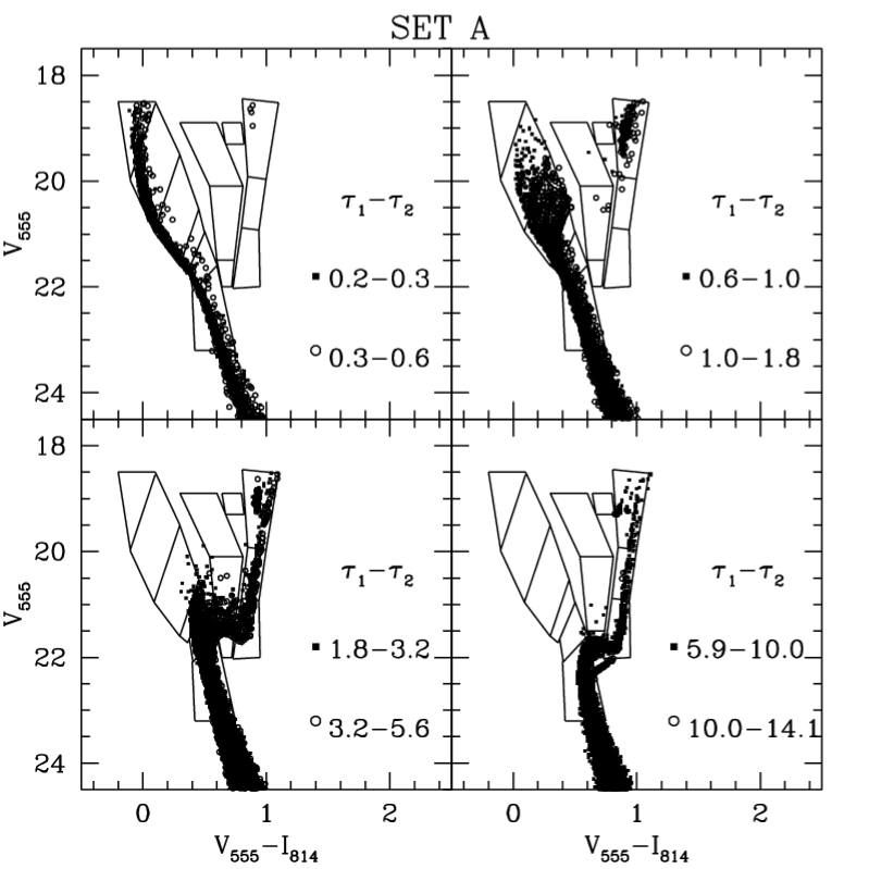
Figure 6: Set A - artificial CMD composed by 8 partial models. Age intervals are showed in Gyrs. Each panel shows two partial models. The regions used in the modelling process are indicated.

The choice of the number of CMD regions in the data $\times$ model comparison was driven by the need to sample different CMD positions while keeping a significant number of stars in each region. We defined $r=13$ CMD regions, which efficiently cover the MS, the subgiant branch (SGB) and the RGB, and which are large enough to contain at least a few tens of stars in a typical observed CMD. These regions will therefore be able to detect the contributions from different populations, i. e., stars with different ages and chemical compositions. Figure 6 shows the chosen CMD regions, along with a synthetic CMD made up of $m=8$ partial models (2 partial models in each panel), whose age ranges are indicated. Most partial models are of younger ages. This choice is due to the fact that CMDs features are more sensitive to younger turn-offs (1 – 6 Gyrs) than to older ones. We also tried other sets of partial models, with $m=7$ and $m=5$. In appendix A we show the results of several control experiments which we used to test the method and its sensitivity to $m$. As a result of these tests, we chose set A (with $m=8$) as the most capable of recovering an unbiased SFH.

5 Results

The CMD modelling method that we adopted followed a regular parameter grid in the SFH: we considered all SFHs possible, by varying the $a_{i}$ ($i=1,8$) coefficients from 0 to 1, in steps of 0.1, and respecting the constraint given by eq. (7). As for the other model parameters, it was impossible to fully explore parameter space. Therefore, we kept the IMF fixed at all times to that from Kroupa (2002) and tested 4 values of E(B-V), 3 values of $\mathrm{f_{bin}=0.25,0.50,0.75}$ and 3 values of $\mathrm{(m-M)_{0}}$ (the one listed in Castro et al. 2001 and the other two by varying it by $\pm$ 0.1). In order to account for LMC depth effects, individual model stars were assigned $\mathrm{(m-M)_{0}}$ values Gaussianly scattered by $\sigma_{(m-M)_{0}}=0.02$ around the model distance. This represents $\simeq\pm 500pc$ distance spread relative to LMC disk mid-point. We considered as our best solution for $\mathrm{E(B-V)}$, $f_{bin}$, $\mathrm{(m-M)_{0}}$ in each field the one that resulted in an absolute $\chi_{\nu}^{2}$ minimum in the entire parameter grid. Our best SFH solution was then the average $a_{i}$ values among those which satisfied the criterion given by eq. 10. We tested the sensitivity of the SFH solution (as well as its $(\chi_{\nu}^{2})_{min}$ value) to $\mathrm{E(B-V)}$, distance modulus and $f_{bin}$. The results are shown in §5.4.

Figures 7 to 9 show the SFHs solutions recovered for the different LMC fields, all of them expressed in terms of $SFH/<SFH>$. As mentioned before, we took the average $SFR/<SFR>$ values within the criterion given by eq. (10) and the 1$\sigma$ deviations from the average as uncertainty bars. A common feature in all recovered SFHs is the existence of a non-negligible old ($\tau>10Gyrs$) population, as had been previously pointed out by Holtzman et al. (1997), Geha et al. (1998), among others. Most SFHs deviate significantly from uniformity, displaying periods of enhanced star formation ($SFR/<SFR>$ $\;\buildrel>\over{\sim}\;$2) and of quiescence (where $SFR/<SFR>$ $\;\buildrel<\over{\sim}\;$0.5).

5.1 NGC1805 and NGC1818

Figure 7: The star formation histories (SFHs) recovered from NGC1805 (top panel) and NGC1818 (bottom panel) fields, using the E(B-V) values that yield the minimum $\chi_{\nu}^{2}$ (E(B-V) = 0.03 and E(B-V) = 0.05 for NGC1805 and NGC1818, respectively). The lines show the average of all values of $\frac{a_{i}}{\bar{a}}$ which satisfy the criterion given by eq. (10). The error bars show the 1$\sigma$ scatter from the average.

In figure 7, top panel, we show our best SFH solution for the field close to NGC1805, obtained with $\mathrm{E(B-V)=0.03}$, $f_{bin}=0.75$ and $\mathrm{(m-M)_{0}=18.59}$. The lower panel shows the result for the field close to NGC1818. The absolute minimum $(\chi_{\nu}^{2})_{min}$ for NGC1818 was found for E(B-V)=0.05, $f_{bin}=0.5$ and $\mathrm{(m-M)_{0}=18.58}$. Both SFHs depicted in Figure 7 are quite distinct from the uniform case. Relatively recent episodes of star formation have occurred in the past $\sim 2$ Gyrs. A broad and significant gap in star formation is present in NGC1805 at $6-10$ Gyrs ago. In NGC1818, our results point to a star formation closer to uniform before $2$ Gyrs ago; the apparent decrease in SFR in the interval $6-10$ Gyrs is still present, but is marginally significant.

5.2 NGC1831 and NGC1868

Figure 8: The star formation histories (SFHs) recovered from NGC1831 (top panel) and NGC1868 (bottom panel) fields, using the E(B-V) values that yield the minimum $\chi_{\nu}^{2}$ (E(B-V) = 0.03 and E(B-V) = 0.00 for NGC1831 and NGC1868, respectively). The lines show the average of all values of $\frac{a_{i}}{\bar{a}}$ which satisfy the criterion given by eq. (10). The error bars show the 1 $\sigma$ scatter from this average.

The best SFH solutions for the fields close to NGC1831 and NGC1868 are drawn in Figure 8. The recovered SFHs for both fields are more consistent with uniformity than the previous two. The quiescent period between $6-10$ Gyrs ago is marginally seen in the NGC 1868 solution and is totally absent in the NGC 1831 field SFH. In the NGC1868 field an increase in star formation in the past $\tau\simeq 1$ – $3$ Gyrs is also apparent. The best values for distance modulus and binary fraction for this field were $\mathrm{(m-M)_{0}}$ = 18.45 and $f_{bin}=0.50$, respectively. For NGC1831, we found $\mathrm{(m-M)_{0}}$ = 18.48 and $f_{bin}=0.75$. The $\mathrm{E(B-V)}$ values corresponding to $(\chi_{\nu}^{2})_{min}$: E(B-V)= 0.03 for NGC1831 and E(B-V)=0.00 for NGC1868.

5.3 NGC2209 and Hodge 11

Figure 9: The star formation histories (SFHs) recovered from NGC2209 (top panel) and Hodge 11 (bottom panel) fields, using the E(B-V) values that yield the minimum $\chi_{\nu}^{2}$ (E(B-V) = 0.11 and E(B-V) = 0.10 for NGC2209 and Hodge 11, respectively). The lines show the average of all values of $\frac{a_{i}}{\bar{a}}$ which satisfy the criterion given by eq. (10). The error bars show the 1 $\sigma$ scatter from this average.

In figure 9 one can find the results for the NGC2209 and Hodge 11 fields. For the first we found E(B-V)=0.11, $\mathrm{(m-M)_{0}}$ = 18.39 and $f_{bin}=0.5$ based on the absolute $(\chi_{\nu}^{2})_{min}$ values, whereas for Hodge 11, our minimization procedure yielded E(B-V) = 0.10, $\mathrm{(m-M)_{0}}$ = 18.34 and $f_{bin}=0.25$. The best SFH solutions for these two fields are similar. They both point to an increase in star formation within the interval $1-6$ Gyrs ago, especially in the case of NGC 2209, where a significant peak is seen at $\tau\simeq 1$ Gyr. Star formation seems to have subdued significantly since then, according to these SFH solutions.

Figure 10: Different star formation histories (SFHs) recovered from the field near NGC1818, resulting from adoption of different $\mathrm{E(B-V)}$ values (panel (a)), $\mathrm{(m-M)_{0}}$ (panel (b)), $f_{bin}$ (panel (c)). (a) The different lines correspond to different choices of $\mathrm{E(B-V)}$: solid - $\mathrm{E(B-V)}=0.05$; dotted - $\mathrm{E(B-V)}=0.03$; dashed - $\mathrm{E(B-V)}=0.04$. (b) The different lines show solutions with different values adopted for $\mathrm{(m-M)_{0}}$: solid - $\mathrm{(m-M)_{0}}=18.58$; dotted - $\mathrm{(m-M)_{0}}=18.68$; dashed - $\mathrm{(m-M)_{0}}=18.48$. (c) The different lines show solutions with different values adopted for $f_{bin}$: solid - $f_{bin}=0.5$; dotted - $f_{bin}=0.75$; dashed - $f_{bin}=0.25$. In all cases, they correspond to the average of all values of $\frac{a_{i}}{\bar{a}}$ which satisfy the criterion given by eq. (10). The error bars show the 1 $\sigma$ scatter from this average.

Figure 11: $(\chi_{\nu}^{2})_{min}$ values recovered from the field near NGC1818, resulting from adoption of different $\mathrm{E(B-V)}$ (panel (a)), $\mathrm{(m-M)_{0}}$ (panel (b)), $f_{bin}$ (panel (c)).

Table 3: The best $\mathrm{E(B-V)}$ are shown in columns $\mathbf{a-d}$ while $\mathrm{(m-M)_{0}}$ values are listed in columns $\mathbf{e,f}$. (a, e) - our results; (b, f) - Castro et al. (2001) results; (c) values quoted by Santiago et al. (2001) for LMC clusters. (d) - Burstein & Heiles (1982) values.

Field	$\mathrm{E(B-V)}$				$\mathrm{(m-M)}$
	$a$	$b$	$c$	$d$	$e$	$f$
NGC1805	0.03	0.04	0.04	0.03	18.69	18.59
NGC1818	0.05	0.04	0.03	0.03	18.58	18.58
NGC1831	0.03	0.0	0.015	0.01	18.48	18.58
NGC1868	0.0	0.02	0.0	0.01	18.45	18.55
NGC2209	0.11	0.07	0.11	0.11	18.39	18.39
Hodge 11	0.10	0.0	–	0.09	18.34	18.34

5.4 Testing the best solution parameters

Our method of CMD modelling yields non-unique solutions for the SFH in a given field; different sets of parameter values often result in acceptable solutions. Figure 10 shows the SFH solutions in the field close to NGC1818 corresponding to different choices of $\mathrm{E(B-V)}$ (panel a), $\mathrm{(m-M)_{0}}$ (panel b) and $f_{bin}$ (panel c). The best values of E(B-V), $f_{bin}$, $\mathrm{(m-M)_{0}}$ and the resulting absolute $(\chi_{\nu}^{2})_{min}$ are quoted on the upper panel. In each panel, we show the sensitivity of the SFH solution to varying one grid parameter at a time. The figure shows that the SFHs vary modestly when model parameter values close to the best solution are considered. Changes in $\mathrm{(m-M)_{0}}$ tend to be more important when one wants to find a meaningful solution for the SFH. Figure 11 shows $(\chi_{\nu}^{2})_{min}$ obtained for NGC1818 with the same parameters whose SFH solutions are presented in figure 10. One can see the behavior of $(\chi_{\nu}^{2})_{min}$ with respect to $\mathrm{E(B-V)}$ (panel a), $\mathrm{(m-M)_{0}}$ (panel b) and $\mathrm{f_{bin}}$ (panel c). It is remarkable that a global $(\chi_{\nu}^{2})_{min}$ was found in this case. The same behaviour is also observed in the other fields.

As described in the previous sections, our choice of best solution was the one which yielded the absolute minimum in $(\chi_{\nu}^{2})$ with respect to $\mathrm{E(B-V)}$, $\mathrm{(m-M)_{0}}$ and $f_{bin}$. We also tested our CMD modelling approach by comparing our best $\mathrm{E(B-V)}$ and $\mathrm{(m-M)_{0}}$ to other values of the same parameter, found independently by other methods. Castro et al. (2001) value of distance modulus was based on a model for the LMC disk, as described in §4.1. Their extinction values were based on isochrone fits to the CMDs of their sample of field LMC stars. Santiago et al. (2001) also applied isochrone fits, but to the observed CMDs of the nearby rich LMC clusters. Since the clusters are 7.3 arcmin from the fields studied here, we assume that any variation in extinction across this distance is negligible. Notice that this assumption may well be wrong in the case of NGC1805, where the broad RGB, seen both in the field and cluster CMDs, may indicate differential redenning. $\mathrm{(m-M)_{0}}=18.50$ was assumed in these isochrone fits for all clusters. Finally, we also use the $\mathrm{E(B-V)}$ values from the Burstein & Heiles (1982) maps, which are based on galaxy counts, for comparison.

Table 3 shows our best $\mathrm{E(B-V)}$ (column $\mathbf{a}$) and $\mathrm{(m-M)_{0}}$ (column $\mathbf{e}$) values provided by the partial models method. In the other columns we show Castro et al. (2001) values for $\mathrm{E(B-V)}$ (column $\mathbf{b}$) and $\mathbf{(m-M)_{0}}$ (column $\mathbf{f}$). The alternative $\mathrm{E(B-V)}$ value by Santiago et al. (2001) is listed in column $\mathbf{c}$. Both works used Padova isochrones from Girardi et al. (2000) in their fits. Burstein & Heiles (1982) $\mathrm{E(B-V)}$ values appear in column $\mathbf{d}$.

There is an excellent agreement among the different determinations of extinction and distance modulus for these fields, especially if we consider the different methods and assumptions that are involved. The only exception is the very low extinction value adopted by Castro et al. (2001) for the field close to Hodge 11, which, according to those authors, should be considered cautiously as a possible result of a wrong distance modulus or mean metallicity adopted for the data.

Finally, we also carried out the same CMD modelling analysis with a cruder version of the chemical-enrichment law presented here in order to test the sensitivity of SFHs to the assumed chemical enrichment. The SFHs show only mild changes but the main characteristics remain, including the existence of field-to-field variations in star formation.

6 Summary and conclusions

In this work we have analyzed 6 deep CMDs of field stars in the LMC using HST/WFPC2 data in the $V_{555}$ and $I_{814}$ filters. Our fields are located from 1.5^∘ to 6$\degr$ from the LMC centre and within $\simeq\,7^{\prime}$ of rich LMC clusters. From 800 to 3500 stars were measured in both V and I bands in each field. We combined these data with those obtained by Castro et al. 2001, carefully placing both datasets in a homogeneous photometric system, which resulted in a much larger photometric sample.

We have studied the behavior of photometric uncertainties and of sample incompleteness in the CMDs. We developed, tested and applied a method to correct for photometric incompleteness as a function not only of magnitude V, but also of (V-I) color.

Based on the final observed CMDs, and with the aid of synthetic model CMDs and objective statistical methods, we have constrained the LMC star formation history. Our synthetic CMDs are capable of incorporating observational effects like extinction, distance modulus, photometric errors and unresolved binarity. For CMD modelling we used the Partial Models Method (Gallart et al. 1999). We have tested the method through control experiments using 3 different sets of partial models. We also examined the sensitivity of our results to adopted distance modulus, binary fraction and extinction.

Although the uncertainty bars are considerable, the recovered SFHs vary from one field to another. The two fields closer to the LMC bar, NGC1805 and NGC1818, show less uniform SFHs, with stronger events of star formation. Star formation peaks are seen in the past $\sim 2Gyrs$. A relatively quiescent phase from $\sim 6$ to $\sim 10$ Gyrs ago is also observed, with significant star formation earlier on. Periods of enhanced star formation at intermediate ages ($\sim 2-6$ Gyrs) are observed in the fields on the eastern side of the LMC, NGC2209 e Hodge 11. The recent star forming activity ($\tau<1$ Gyr) seen in NGC1805 and NGC1818 is no longer observed. Finally, a more uniform star formation history results from CMD modelling of the fields in the NW part of the LMC disk, NGC1831 and NGC1868, especially in this first. The only important variation from a uniform SFR in NGC1868 is possibly an enhanced star formation period from $\tau\simeq 1$ to $\tau\simeq 3$ Gyrs. In all fields, one can clearly observe the significant contribution of older populations ($\tau$ $\;\buildrel>\over{\sim}\;$$6$ Gyrs) to their CMDs.

In brief, we can partially relate the recovered SFHs to fields position: fields near the LMC bar (NGC1805 and NGC1818) present more recent star formation ($\tau$ $\;\buildrel<\over{\sim}\;$$1-2Gyrs$), something that is actually confirmed by a larger number of upper MS stars on their observed CMDs. NGC2209 and Hodge 11, located to the east of the LMC center, show little recent star formation, but display an excess of intermediate age ($\tau\sim 2-6$ Gyrs) stars. Finally, NGC1831 and NGC1868 are a further step closer to a uniform SFH, although some increase in star formation in the last $\simeq 3$ Gyrs is also visible in the NGC 1868 field.

It is important to recognize that the inferred SFHs do not describe the star formation rates that took place in situ, for the stars currently found in our HST/WFPC2 fields have certainly dispersed away from their various formation sites. Therefore, the periods of enhanced formation we find should reflect star formation rates over much broader regions of the LMC, perhaps the entire galaxy in the case of the older populations. The same applies to the intervals of lower than average activity. The observed differences from one field to the other show that the mixing of stellar populations within the LMC field is not 100% efficient; on the contrary, there exist coeval stars, resulting from the same burst, which move coherently in the galaxy’s potential, regardless of their ages or original location. A dynamical model, taking into account typical velocity dispersions and orbital motions, is then required in order to reconstruct the star formation sites, burst time-scales and locations, from our resulting SFHs.

This work gives continuity to a historical process of recognition of the importance of old and intermediate-age populations in the LMC. Until the beginning of the 80s, the LMC was seen as being formed of relatively young stars (Butcher 1977, Stryker 1984). In the beginning of the 90s, Bertelli et al. (1992) and Vallenari et al. (1996) suggested a star formation burst at $\tau\sim$ 4 Gyr and found evidence for some spatial variation in the star formation. The HST observations revealed a considerable portion of intermediate-age and old stars. The recent reconstructed SFHs lead us to conclude that stars older than 4 Gyr are at least as numerous as younger ones (Holtzman et al. 1997, Geha et al. 1998). Our results clearly corroborate this notion.

Another important result is that the gap in star formation in the LMC is not seen in the SFHs derived here; evidence for a decrease in the SFR in the interval $6-10$ Gyrs is seen only in the fields closer to the LMC bar. It is therefore hard to reconcile the SFH of fields stars with the observed age distribution of LMC clusters, which reveals a longer and older age gap.

It is important to remember that we have always used the same chemical enrichment model which is consistent with metallicities and ages of LMC clusters (Olszewski et al. 1996). However, there is evidence, including from the present work, that the field stars SFH differs from the SFH of the LMC clusters (Holtzman et al. 1999). Thus, it would be extremely important to obtain direct and strong constraints on the chemical enrichment of LMC field stars (Cole et al. 2000, Smecker-Hane et al. 2002). For this challenge one needs the new generation telescopes, such as GEMINI and SOAR.

Appendix A Control Experiments

In order to implement the PMM, we need to define the number of partial models to use, $m$, and to check the efficiency of the method. This is done by generating an artificial CMD based on some known input SFH, as described in Sect. 4.1, and submitting this CMD to the modelling process described in Sect. 4.2. In other words, we compare this “artificial data” CMD with other artificial CMDs created in the same way but following alternative schemes of SFH. This comparison makes use of the PMM, with different choices of $m$. The results of such control experiments can be viewed in figures 12–14. In these figures, the panels along each horizontal line refer to the results of a given set of partial models. We tested three sets: A ($m=8$), B ($m=7$) and C ($m=5$). The vertical columns of the panels correspond to a given input SFH. The input SFH is given as a solid line in each panel. It varies slightly from one set to the other because of the variation in the age intervals covered by each set. The best solution, as described in §5, and which uses the quality criterion given in §4.2, is shown as open circles. The open triangles correspond to the sets $\{a_{i}\}$ that yield $(\chi_{\nu}^{2})_{min}$, i.e., the minimum $(\chi_{\nu}^{2})$ value among all $\{a_{i}\}$ sets. This $(\chi_{\nu}^{2})_{min}$ value is given in each panel. The figures show a total of 9 input SFHs, 3 per figure.

In most cases, the recovered SFHs (either the best or minimum solution) are very similar to the input ones, which shows that the method is in fact capable of reconstructing a SFH from CMD data. However, some discrepancies significantly beyond the error bars are seen in a few points, especially in panels A.2.c, A.2.f, A.3.a, A.3.d, A.3.f. In most these cases, only one point along the SFH is not well recovered, as is the case of the underestimate in star formation rate (SFR) at $\tau\simeq 8$ Gyrs in panel A.2.c. This latter panel actually shows a situation (for $\tau\simeq 0.5$ Gyr) where the best solution is a good description of the input model, whereas the minimal solution is not. This is also seen in panels A.3.b and A.3.e. We thus conclude that the adoption of an average solution over some range in $(\chi_{\nu}^{2})$ close to the minimum, as in our best solution, rather than the minimum itself, results in more stable results. Another conclusion is that SFHs dominated by a single burst tend to be more easily reproduced, while more complex or nearly constant star formation input scenarios often result in recovered SFHs with misplaced peaks (A.3.a, A.3.c and A.3.f) or slightly distorted SFH shapes (as in A.2.c, A.3.b, A.3.e, A.3.h). Based on the general results from these control experiments, and considering the relative frequency of discrepancies between input and recovered SFRs, we decided to use set A of partial models, with $m=8$; this set shows about the same number of discrepant points as set B ($m=7$) and set C ($m=5$), but samples better the SFH.

Figure 12: Each column shows SFH schemes given in $\mathrm{SFR/<SFR>}$ (solid lines) and corresponding recovered SFH (open circles). Each line shows the results for each set of partial models: set A (panels (a), (b) and (c)); set B (panels (d), (e) and (f)) and set C (panels (g), (h) and (i)). The set of $a_{i}$ values obtained on best solution (i. e. $(\chi_{\nu}^{2})_{min}$). Error bars show acceptable $a_{i}$ values with dispersion within $1\sigma$.

Figure 13: Same as shown in figure 12, but for the other 3 SFH schemas.

Figure 14: Same as shown in figure 12, but for the other 3 SFH schemas.