[astro-ph/0412522] Interferometry and the study of binaries

1 Introduction

The study of binaries has a number of goals. To introduce these, let us look at the evolution of the binary shown in Figure 1. The initial binary consists of stars with masses of 15 and 7 $M_{\odot}$ , in an orbit of 200 d. The more massive star evolves fastest, ascends the giant branch and transfers its envelope to its companion (b-d). During this process, the size of the orbit changes due to conservation of angular momentum. The denuded core of the initially most massive star continues to evolve and via a supernova event forms a neutron star (e). The companion to the neutron star through accretion has gained mass and angular momentum, and has thereby turned into a Be star. When this star evolves in turn, it engulfs the neutron star (f-g). The envelope is expelled as the neutron star moves in. At the end the neutron star forms a close binary with the helium core. This core in turn becomes a neutron star via a supernova event, and thus a binary of two neutron stars may be formed (h).

In general it is thought that the full evolution of any binary is set by the initial conditions, in particular the two masses and the orbital period. If the supernova event imparts an appreciable velocity to the neutron star in an arbitrary direction, an element of uncertainty is introduced, which means that the evolution following a supernova event can only be described statistically. Other factors of interest, but generally less dramatic in importance, are the initial eccentricity of the orbit, the chemical composition of the stars, and their initial rotation. If one would know the distribution of all these properties for newly formed binaries, one could synthesize a population of binaries in our galaxy as follows. In step one, one chooses randomly from the initial distributions a realization of the binary, i.e. in particular a mass for the more massive star, a mass for the less massive star, and the orbital period. One then computes the evolution of this binary and keeps track of all its different stages. This procedure is repeated until a sufficiently large number of binary evolutions is available. The sum of all this provides the current population of binaries in our galaxy, for a stationary birth rate. If one is interested in relatively old binaries, one must weigh the numbers of binaries of different age using the history of the star formation rate.

From this we can derive three important questions that the study of binaries tries to answer.

•

what are the distributions of the parameters of binaries at birth, in particular of the primary mass $M_{1}$ , secondary mass $M_{2}$ and orbital period $P_{b}$ ? This question relates closely to the formation of stars.
•

how do binaries evolve? This question includes the evolution of single stars, as well as processes typical for binaries, such as mass transfer and tidal interaction. It relates to the evolution of the radius of a star with time, to the occurrence of special processes (type Ia supernovae, gamma-ray bursts), and to the enrichment and energetics of the interstellar medium.
•

what do we learn from individually interesting systems? As an example, accurate measurements of masses of neutron stars constrain the equation of state at nuclear densities (which determines the maximum possible mass for a neutron star).

Before discussing these topics, we first explain how interferometry helps to obtain information about a binary.

2 How to study a binary?

The orbital period $P_{b}$ and the semi-amplitude of the radial velocity $K_{1}$ of star 1 in a binary provide an equation, called the mass function, for three unknowns: the masses $M_{1}$ and $M_{2}$ and the inclination $i$ of the binary with respect to the line of sight ( $i=90^{\circ}$ for edge-on):

{P_{b}{K_{1}}^{3}\over 2\pi G}\left(1-e^{2}\right)^{3/2}={(M_{2}\sin i)^{3}\over(M_{1}+M_{2})^{2}}

(1)

Here $G$ is the gravitational constant, and $e$ the orbital eccentricity, which is determined from the radial velocity curve (sinusoidal for $e=0$ ). We thus require two more equations for the three unknowns. In a double-lined binary, one such equation is the mass function for star 2. We see that by dividing the two mass functions, we obtain the mass ratio $q\equiv M_{2}/M_{1}=K_{1}/K_{2}$ . This leaves $i$ as an unknown. There are various methods to determine $i$ , but in general the most accurate method is to measure the visual relative orbit (Fig. 2). As a bonus, this measurement also provides us with the distance to the binary (from the comparison of astrometric velocities [ ${}^{\prime\prime}/s$ ] and velocities from the spectra [km/s]). The distance is required if we wish to determine the radii of the stars. In a single-lined binary, all parameters ( $M_{1}$ , $M_{2}$ , $i$ ) can be solved if we can measure the orbits of the two stars separately. For a more exhaustive list of possible ways to study a binary see Quirrenbach (2001).

For the radii of the stars we can use the methods used for single stars, provided we can separate their images, c.q. determine the flux of each star separately.

Refer to caption — Figure 2: Visual orbit (left) and radial velocities (right) for a naked T Tauri star (045251+3016) in the Taurus Auriga star forming region. Note that even with a rough visual orbit, the inclination is accurately determined, at 113.8 ${}^{\circ}\pm$ 3.4^∘. Also note that once the radial velocity curve of one star is well determined, the other one can be fixed with one or two accurate measurements (indicated $\circ$ ). After Steffen et al. (2001).

Radial velocities are high in close binaries, separate images of the binary stars are easiest made of wide binaries (Fig. 3). Due to improved accuracy in the measurements of radial velocities on one hand, and to higher spatial resolution in imaging, the number of spectroscopic binaries for which visual orbits can be determined is increasing. It is here that interferometry helps. Interferometry may produce a direct image of the binary. A nice example is the bispectrum speckle interferometry with the SAO 6 m telescope of OB stars in the Orion nebula cluster (Schertl et al. 2003 and references therein). By doing this over a long period of time, one can produce the relative visual orbit. An example from the HST Fine Guidance Sensor is the orbit of a naked T Tauri star in the star-forming regions of Taurus-Auriga (Steffen et al. 2001, see Fig. 2). It is important to note, however, that actual imaging is not necessary: one can also fit the observed visibilities directly. A good example is the analysis of 64 Psc with the Palomar Testbed Interferometer (Boden et al. 1999). This method has the advantage that shorter observations can be used.

The examples given above are arbitrarily chosen: an extensive catalogue of visual orbits is maintained by Hartkopf & Mason at http://ad.usno.navy.mil/wds/orb6.html; see also Hartkopf et al. (2001).

3 The initial parameters of newly born binaries

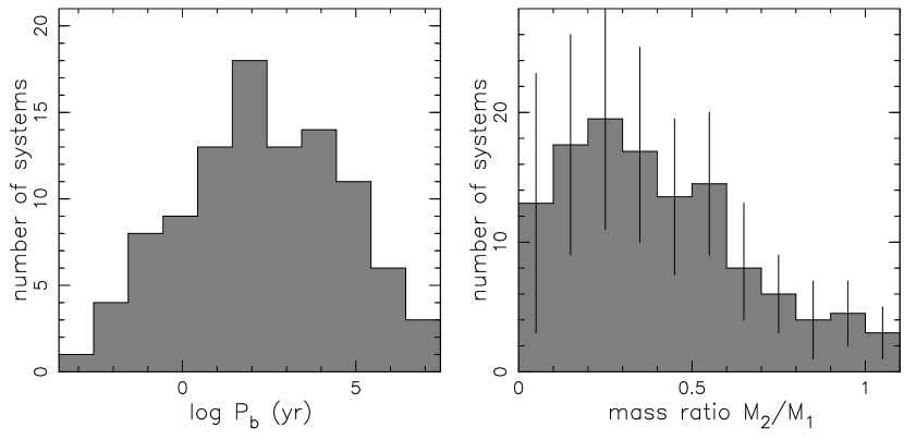
Duquennoy & Mayor (1991) published an extensive study of the initial parameters of G stars, derived from observations of 164 main-sequence F7-G9 stars. They find for example that the period distribution is given by a log-normal distribution. Due to relatively large errors, the distribution of mass ratios is less constrained (Fig. 4). One would like to obtain distributions with equal accuracy for the other spectral types.

Mathematically the distribution of initial masses $M_{1}$ and $M_{2}$ and the orbital periods $P_{b}$ can be written as a probability function $\Pi(M_{1},M_{2},P_{b})$ . It is tempting to assume that this combined probability function can be separated into separate probabilities for the masses and period, i.e. $\Pi(M_{1},M_{2},P_{b})=\Pi(M_{1})\Pi(M_{2})\Pi(P_{b})$ , or alternatively for the mass ratio $q\equiv M_{2}/M_{1}$ that $\Pi(M_{1},q,P_{b})=\Pi(M_{1})\Pi(q)\Pi(P_{b})$ . From the limited observations that we have we already know that this is not the case:

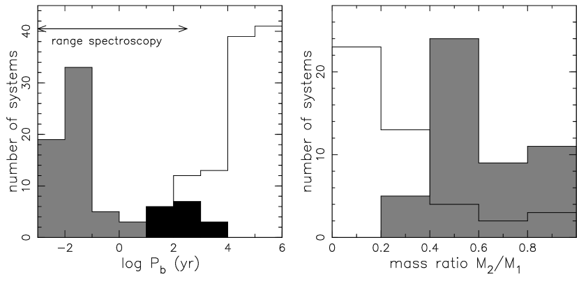
\Pi(M_{1},q,P_{b})\neq\Pi(M_{1})\Pi(q)\Pi(P_{b});\qquad q\equiv M_{2}/M_{1}

Compare for example the distributions for O stars (Fig. 3) and for G stars (Fig. 4). The period distribution of G stars peaks at $\sim 100$ yr; the mass-ratio distribution at low values. These distributions are not compatible with the distribution for spectroscopic O-star binaries, even if we take into account the selection effects which prevent us from measuring binaries with extreme mass ratios ( $M_{2}<0.2M_{1}$ , say) spectroscopically (there aren’t enough O stars left to change the distributions much). On the other hand, O stars in wide binaries more often have low-mass companions. Thus $\Pi(q)$ may depend both on the primary mass $M_{1}$ and on the orbital period $P_{b}$ .

The consequence of this is that one will need to study many binaries before the general distribution of initial parameters can be determined with some accuracy. However, for the study of binary evolution one may concentrate on binaries with primaries that evolve within the Hubble time, i.e. with masses $M_{1}>0.8M_{\odot}$ (spectral type G V or earlier), and in which the stars influence one another, i.e. with binary periods $P_{b}<50$ yr. The other binaries either don’t evolve at all, or if they do, the two stars evolve essentially independently from one another.

With Kepler’s law and the definition of the parsec, we may write the semimajor axis $a$ of a binary, expressed in milliarcseconds, in terms of the total mass $M\equiv M_{1}+M_{2}$ , orbital period $P$ and distance $d$ as

{a\over{\mathrm{m}as}}=\left({M\over M_{\odot}}\right)^{1/3}\left({P\over 1{\rm yr}}\right)^{2/3}\left({d\over 1{\mathrm{k}pc}}\right)^{-1}

(2)

$a$ changes only slowly with mass – a range of a factor 10 in $M$ corresponds to a range of 2 in $a$ . I will give $a$ according to this equation as the required resolution, but the reader should note a) that to resolve the orbit projected on the sky one would typically need to measure separations down to $\sim 0.2a$ , say; and b) that the visibility doesn’t have to be measured down to zero to measure a separation (I thank F. Delplancke for reminding me of this).

To obtain a sufficiently large sample of low-mass stars, of spectral types AFGKM, it is enough to reach relatively nearby stellar clusters, including star formation regions, at a distance of $\sim 130$ pc, say. With $M\simeq M_{\odot}$ we see from Eq. 2 that an orbit of 100 d is resolved with 3 mas at 130 pc; or with 1 mas at 400 pc. A G0 V star has $K\simeq 11$ at 400 pc; an A0 V star $K\simeq 8.5$ . To obtain a sufficiently large sample of OB stars, one needs to study clusters out to about a kpc; this includes the clusters of the Gould Belt. At 1 kpc and for $M=20M_{\odot}$ , 3 mas resolves an orbit of 1 yr; and 1 mas an orbit of 0.2 yr.

In Fig. 5 we plot the visual and K-band magnitudes of main-sequence stars; from the figure we see that detection of a companion with one-tenth of the mass of the primary requires a magnitude contrast of 5-6 in $V$ and slightly less in $K$ . A large magnitude difference makes it more difficult to obtain radial velocities of both stars. It is therefore useful to note that low-mass pre-main-sequence stars are relatively bright, and easier detected. As an example, we see in Fig. 6 that on the main-sequence a 1.5 $M_{\odot}$ star is a factor 25 more luminous than an 0.8 $M_{\odot}$ star; but only a factor 2 when both stars are 1 Myr old. To study binaries with extreme mass ratios one may therefore wish to study star-forming regions.

Improving the resolution of the interferometers by a factor three with respect to the current resolution increases the number of available orbits by an order of magnitude for O stars (which are in the galactic plane and therefore have a two-dimensional spatial distribution), and more for the less massive stars (which form a thicker disk).

4 Tests on stellar evolution

Once we have the parameters of both stars in a binary, we can apply tests of stellar evolution. The more direct tests are done in a binary where the stars have not yet influenced one another, and have evolved essentially independently. We discuss two examples.

The analysis of radial velocities and the visual orbit of the pre-main-sequence binary
RXJ 0529.4+0041 (the RX indicates that the binary is a Rosat X-ray source) give masses of $1.25M_{\odot}$ and $0.91M_{\odot}$ , with errors of $0.05M_{\odot}$ . We see in Fig. 6 that the mass derived for the primary from evolutionary tracks is marginally higher; and that the positions of the stars in the Hertzsprung-Russell diagram are compatible with both stars being about 5 Myr old (Covino et al. 2000).

The stars in HR 6902 have masses $(3.86\pm 0.15)M_{\odot}$ and $(2.95\pm 0.09)M_{\odot}$ , respectively. The less massive star is still on the main-sequence, the more massive star has already evolved into a late-type giant (Fig. 6). The locations of the stars in the Hertzsprung-Russell diagram is compatible with the evolutionary tracks for stars of these masses only if overshooting is assumed (i.e. the gas that rises with convection moves a little bit beyond the boundary given by the Schwarzschild criterion for convection). HR 6902 thus proves the importance of overshooting (Schröder et al. 1997). A star of 3 $M_{\odot}$ with the nominal luminosity of the secondary (indicated in the Figure with a $\bullet$ ) has an age of about 260 Myr, which is older than the full evolution of a star of 4 $M_{\odot}$ . Only if the luminosity of the secondary is less, is its age compatible with the age of the primary. E.g. a star of 3 $M_{\odot}$ reaches $L=100L_{\odot}$ (well within the measurement accuracy) after 170 Myr.

Whereas tests on non-interacting stars are more or less straightforward, it is more difficult to constrain processes like loss of mass and angular momentum from the binary. An example of such a test is the one on the binary AS Eri. This is an Algol-type binary, i.e. a binary in which a giant transfers mass to a more massive unevolved star. The giant must originally have been the more massive star, but has become less massive than its companion by transferring mass to it or by losing mass which then leaves the binary. Refsdal et al. (1974) have shown that the current component masses and orbital period of AS Eri imply that the binary must have lost a significant amount of angular momentum during the mass transfer, presumably with a significant loss of mass.

In Figure 1 we can assign several other areas of binary evolution where more knowledge is required. Single stars lose mass in the form of a stellar wind; what is the effect of this in a binary (in e.g. phases a-b and e-f)? Does it indeed, as is often assumed, widen the binary? Is the stellar wind stronger when a star comes close to its Roche lobe (Tout & Eggleton 1988)? Is mass transfer between the stars accompanied by loss of mass from the binary (phases b-d)? What happens exactly when the mass tranfer is dynamically unstable? Do we indeed get a spiral-in (phases f-g)? In general, the answers to questions like these can be sought on one hand in the study of carefully selected binaries – like AS Eri – and on the other hand by the statistical study of large numbers of binaries, combined with population synthesis.

5 Triple and multiple systems

Perhaps the first thing to note about triple and multiple systems is that they are common! Several naked eye stars are very complex systems. An example is Castor ( $\alpha$ Gem) which consists of three stars, each of which is a binary (Heintz, 1988): Castor A, a binary of an A star with an unknown companion in a period of 2.9 d is in an orbit of 467 yr with Castor B, a binary of an A star with unknown companion in an orbit of 9.2 d; this quadruple system is in a $\sim$ Myr orbit around Castor C, a binary of two M dwarfs in a 19.8 hr orbit. It is remarkable that the companions of the A stars in Castor A and B have not been detected so far.

The detailed study of the nearby cluster Praesepe finds a ratio of single to binary to triple stars as $s:b:t=47:30:3$ , i.e. of 115 stars, 60 are in a binary and 9 in a triple (Mermilliod & Mayor 1999; see also Mermilliod et al. 1994, with a list of triple stars in several clusters). A speckle interferometry study of the O stars in the Trapezium of the Orion nebula finds 1.75 companions per primary, on average, again indicating a high incidence of multiple systems (Weigelt et al. 1999). And finally, continued study of radial-velocity orbits of close binaries in the field indicates that a sizable fraction of them probably are part of multiple systems (Mayor & Mazeh 1987).

The stability of triple stars has been the subject of much research. In general, a three-body system is not stable unless it is hierarchical, i.e. two stars form a binary which is much closer than the distance to the third star. Thanks to some brilliant mathematics by Mardling (2001) a simple criterion is now available to determine the stability of any coplanar triple system (see also Sect. 4 of Mardling & Aarseth 2001).

An interesting aspect of triple systems has recently been discussed by Muterspaugh et al. (2004; see also Lane & Muterspaugh 2004). $\kappa$ Peg is a triple in which a 5.97 d binary ( $\kappa$ Peg B) is in a 11.6 yr orbit with a third star ( $\kappa$ Peg A). The outer orbit has a projected size of about 0.4^′′, and is easily resolved with the Palomar Testbed Interferometer. The distance between the two stars A and B is determined to a precision of about 40 $\mu$ as: since the short-period binary has a projected semimajor axis of almost 1 mas, the observations provide a visual orbit for the short-period binary (Fig. 7).

In general then, it appears possible to resolve a binary with a size smaller than the resolution of an interferometer, provided that there is a sufficiently nearby third star that is used as a reference. This third star may be in a triple with the binary; but the method does not require this.

An example of a target that will be accessible to a future interferometer with $\sim$ mas resolution is the blue straggler S 1082 in the old open cluster M 67 (Van den Berg et al. 2001). This star is in fact a triple, in which a 1.07 d eclipsing binary of stars with masses 2.7 and 1.7 $M_{\odot}$ is in an orbit of $\sim$ 3 yr with a third star of $\sim 1.7M_{\odot}$ . Both the primary in the inner binary and the third star are blue stragglers of their own account. With Eq. 2 we see that the outer and inner orbits have semimajor axes of about 5 mas and 40 $\mu$ as, respectively.

6 Binaries with neutron stars or black holes

Visual orbits would be very useful for the study or X-ray binaries in which a neutron star or black hole accretes matter from a companion (for a recent review, see Charles & Coe 2004). Even in systems in which eclipses or ellipsoidal flux variations give an indication of the inclination of the orbit, the actual value of the inclination is often very uncertain. Thus, a visual orbit and with it a more accurate inclination will help to improve the accuracy of the mass determination.

Consider for example the well-studied X-ray binary Cyg X-1, in which a black hole accretes mass from a high-mass O star. Extensive optical studies cannot constrain the inclination more accurately than a range from 28^∘ to 38^∘, corresponding to a range of the mass of the black hole of 20 to 10 $M_{\odot}$ (Gies & Bolton 1986). For a total mass $\sim 50M_{\odot}$ , orbital period of 5.6 d and a distance $\simeq 2$ kpc, the semimajor axis of the orbit is about 0.1 mas. Similarly, the inclination of the 9 d orbit of Vela X-1 may range from 73^∘ to 90^∘ allowing masses of the neutron star between 1.8 and 2.0 $M_{\odot}$ and of its O star companion between 23 and 26 $M_{\odot}$ (Barziv et al. 2001). At a distance of 1.4 kpc the semimajor axis is 0.18 mas.

As an example of a black hole that accretes from a less massive donor, we consider the widest system GRS 1915+105: a (14 $\pm$ 4) $M_{\odot}$ black hole accreting from a $\sim 1M_{\odot}$ star in an orbit of 34 d (Greiner et al. 2001). At a distance of 10 kpc the semimajor axis is 0.05 mas. A relatively nearby low-mass X-ray binary is Sco X-1, in which a neutron star forms a 19 hr binary with a low-mass donor. At a distance of 2.8 kpc (Bradshaw et al. 1999) its semimajor axis is about 0.01 mas.

We see that to study X-ray binaries, interferometers will have to reach accuracies down to fractions of a milliarcsecond. For the high-mass systems, magnitudes are not a problem ( $V=8.9$ for Cyg X-1, and $V=6.9$ for Vela X-1). The low-mass systems are much less bright in the optical ( $K\simeq 13$ for GRS 1915+105 and $V=12.4$ for Sco X-1). However, the study of these binaries with interferometry will be complicated by their intrinsic strong variability, and by the fact that the size of the stars is about half of the distance between them. For the low-mass binaries, both objects (mass donor and accretion disk) have comparable fluxes in the visual, but in high-mass binaries the accretion disk is very much fainter than the O or B star donor.

The systems discussed so far have donors that fill their Roche lobe in relatively short orbital periods. Although less conspicuous in X-rays than these systems, the majority of high-mass X-ray binaries may actually be Be stars that irregularly transfer mass to a neutron star in much wider orbits (see Fig. 1e). These systems are being discovered in increasing numbers as transient bright sources of X-rays (see catalogue by Liu et al. 2000). With a typical mass of $\sim 15M_{\odot}$ , a period of a year, and a distance of 2.5 kpc, a semimajor axis of 1 mas follows. The transient nature of these sources implies that the interferometry must be performed during an outburst, i.e. as a target-of-opportunity.

Low-mass X-ray binaries may evolve into relatively wide binaries in which a radio pulsar is accompanied by an undermassive (i.e. 0.2-0.4 $M_{\odot}$ ) white dwarf. Since the neutron star doesn’t emit detectable optical radiation, the motion of the white dwarf can only be measured against a third object. Binaries of this type occur in globular clusters, where third objects are certainly available. An interesting example is PSR 1620 $-$ 26, an 11 ms pulsar in a 191 d orbit with an 0.3 $M_{\odot}$ white dwarf, in the globular cluster M 4 (Sigurdsson et al. 2003, and references therein). Its semimajor axis at the cluster distance of 2.2 kpc is 0.37 mas. The problem with this system is its extreme faintness, at $V=24$ .

In conclusion we may say that the study of compact stars in binaries requires a resolution well below a milliarcsecond. This is true not only for the binaries with neutron stars and black holes that we discussed above, but also for the white dwarfs accreting from a low-mass donor star in cataclysmic variables. A well-studied example is SS Cyg, at about 160 pc (Harrison et al. 1999). Its semi-major axis corresponds to 0.06 mas.

7 Closing remarks

A next generation of interferometers, which can resolve binaries down to the milliarcsecond level, will be able to determine the visual orbits of enough binaries (several thousand) to determine the properties (masses, orbital period) with which young binaries are born. This requires a very large observing programme (comparable to e.g. the CORAVEL survey), and thus probably a dedicated telescope. The number of observations may be limited, first by limiting the survey to binaries that evolve within the Hubble time, i.e. with primary masses higher than 0.8 $M_{\odot}$ , and that are close enough that the stars may affect one another’s evolution, i.e. with orbital periods less than 30-50 yr. Also, by selecting binaries with known orbital periods and orbital phases, one may be able to time the interferometric observations cleverly for faster results. Such binaries could be found in clusters of stars, where multi-object spectroscopy would be efficient in determining large numbers of orbits.

Knowledge about the evolution of binaries may be more difficult to obtain; on the other hand, by selecting specific binaries one can obtain interesting results with a relatively small programme.

The study of X-ray binaries requires such small resolution for stars often very faint that it may not be possible with the next generation of instruments. In some cases, indirect resolution of an orbit by use of a third star may be possible.

A question which will have to be adressed is in how far the GAIA satellite will already adress the questions of binary formation and evolution. Its fantastic resolution (down to 3 $\mu$ as) and very large number (10⁹) of observed stars make this an important mission for binary studies (e.g. Zwitter & Munari 2004). Especially large-scale programmes for groundbased interferometry should be aimed to complement, rather than duplicate, the GAIA results.

References

Barziv, O., Kaper, L., van Kerkwijk, M., Telting, J., & van Paradijs, J. 2001, A&A, 377, 925

Binney, J. & Merrifield, M. 1998, Galactic Astronomy (Princeton University Press)

Boden, A., Lane, B., Creech-Eakman, M., et al. 1999, ApJ, 527, 360

Bradshaw, C., Fomalont, E., & Geldzahler, B. 1999, ApJ, 21, L121

Charles, P. & Coe, M. 2004, in Compact stellar X-ray sources, ed. W. Lewin & M. van der Klis (Cambridge University Press), in press (astro-ph/0308020)

Covino, E., Catalano, S., Frasca, A., et al. 2000, A&A, 361, L49

d’Antona, F. & Mazzitelli, I. 1994, ApJS, 90, 467

Duquennoy, A. & Mayor, M. 1991, A&A, 248, 485

Gies, D. & Bolton, C. 1986, ApJ, 304, 371

Greiner, J., Cuby, J., & McCaughrean, M. 2001, Nature, 414, 522

Harrison, T., McNamara, B., Szkody, P., et al. 1999, ApJ, 515, L93

Hartkopf, W., Mason, B., & Worley, C. 2001, AJ, 122, 3472

Heintz, W. 1988, PASP, 100, 834

Lane, B. & Muterspaugh, M. 2004, ApJ, 601, 1129

Liu, Q.-Z., van Paradijs, J., & van den Heuvel, E. 2000, A&AS, 147, 25

Mardling, R. 2001, in Evolution of Binary and Multiple Star Systems, ed. P. Podsiadlowski & et al., ASP Conference Series 229, 101

Mardling, R. & Aarseth, S. 2001, MNRAS, 321, 398

Mason, B., Gies, D., Hartkopf, W., Bagnuolo, W., ten Brummelaar, T., & McAlister, H. 1998, AJ, 115, 821

Mayor, M. & Mazeh, T. 1987, A&A, 171, 157

Mermilliod, J.-C., Duquennoy, A., & Mayor, M. 1994, A&A, 283, 515

Mermilliod, J.-C.and Mayor, M. 1999, A&A, 352, 479

Muterspaugh, M., Lane, B., Burke, B., Konacki, M., & Kulkarni, S. 2004, SPIE Conference: New Frontiers in stellar interferometry, 5491, in press (astro-ph/0407088)

Quirrenbach, A. 2001, in The formation of binary stars, IAU Symposium 200, ed. H. Zinnecker & R. Mathieu (ASP), 539–546

Refsdal, S., Roth, M., & Weigert, A. 1974, A&A, 36, 113

Schertl, D., Balega, Y., Preibisch, T., & Weigelt, G. 2003, A&A, 402, 267

Schröder, K.-P., Pols, O., & Eggleton, P. 1997, MNRAS, 285, 696

Sigurdsson, S., Richer, H., Hansen, B., Stairs, I., & Thorsett, S. 2003, Science, 301, 193

Steffen, A., Mathieu, R., Lattanzi, M., et al. 2001, AJ, 122, 997

Tout, C. & Eggleton, P. 1988, MNRAS, 231, 823

van den Berg, M., Orosz, J., Verbunt, F., & Stassun, K. 2001, A&A, 375, 375

Verbunt, F. 1993, ARA&A, 31, 93

Weigelt, G., Balega, Y., Preibisch, T., et al. 1999, A&A, 347, L15

Zwitter, T. & Munari, U. 2004, Rev. Mex. A.A. 21, 251