Ram pressure stripping of disk galaxies

Galaxies in clusters and groups moving through the intracluster or intragroup medium (abbreviated ICM for both) are expected to lose at least a part of their interstellar medium (ISM) by the ram pressure they experience. We perform high resolution 2D hydrodynamical simulations of face-on ram pressure stripping (RPS) of disk galaxies to compile a comprehensive parameter study varying galaxy properties (mass, vertical structure of the gas disk) and covering a large range of ICM conditions, reaching from high density environments like in cluster centres to low density environments typical for cluster outskirts or groups. We find that the ICM-ISM interaction proceeds in three phases: firstly the instantaneous stripping phase, secondly the dynamic intermediate phase, thirdly the quasi-stable continuous viscous stripping phase. In the first phase (time scale 20 to $200\,\textrm{Myr}$) the outer part of the gas disk is displaced but only partially unbound. In the second phase (10 times as long as the first phase) a part of the displaced gas falls back (about 10% of the initial gas mass) despite the constant ICM wind, but most displaced gas is now unbound. In the third phase the galaxy continues to lose gas at a rate of about $1\,M_{\sun}\,\,\textrm{yr}^{-1}$ by turbulent viscous stripping. We find that the stripping efficiency depends slightly on the Mach number of the flow, however, the main parameter is the ram pressure. The stripping efficiency does not depend on the vertical structure and thickness of the gas disk.

We discuss uncertainties in the classic estimate of the stripping radius of Gunn & Gott (1972), which compares the ram pressure to the gravitational restoring force. In addition, we adapt the estimate used by Mori & Burkert (2000) for spherical galaxies, namely the comparison of the central pressure with ram pressure. We find that the latter estimate predicts the radius and mass of the gas disk remaining at the end of the second phase very well, and better than the Gunn & Gott (1972) criterion.

From our simulations we conclude that gas disks of galaxies in high density environments are heavily truncated or even completely stripped, but also the gas disks of galaxies in low density environments are disturbed by the flow and back-falling material, so that they should also be pre-processed.

1 Introduction

The differences observed between disk galaxies in clusters and in the field indicate that the evolution of galaxies is not only ruled by interior processes, but also strongly by the galaxy’s environment. Some cluster galaxies show distortions in their gas components as well in as their stellar disks. These examples can be explained by tidal interactions with some fellow cluster members (mergers or harassment, see review by Mihos 2004 and references therein). However, a number of galaxies have rather normal stellar disks but truncated gas disks (e.g. NGC 4522: Kenney & Koopmann 1999, 2001,Vollmer et al. 2004b; NGC 4548: Vollmer et al. 1999; NGC 4848: Vollmer et al. 2001a). Cayatte et al. (1990, 1994) observed the brightest spiral galaxies in the Virgo cluster and found the trend that the galaxies closest to the cluster centre have the smallest HI disks. In general, cluster spirals are HI deficient compared to their field relatives. They are more deficient near the cluster centre (Solanes et al. 2001), but deficient galaxies can be observed out to large distances (2 Abell radii) from the cluster centre (Solanes et al. 2001). HI deficient galaxies tend to be on more radial orbits which lead them deeper into the cluster. Koopmann & Kenney (1998, 2004a, 2004b) studied the star formation rates in Virgo spirals and found that also the star formation of many cluster members is truncated, that means it is suppressed significantly in the outer regions, but normal or even enhanced in the central region of the galaxy.

The combination of an intact stellar disk but truncated gas disk can hardly be achieved by tidal interactions, as this usually also disturbs the stellar component. But even if a cluster galaxy does not interact with another galaxy, it still moves through the intra-cluster medium (ICM) and experiences a ram pressure $p_{\mathrm{ram}}\approx\rho_{\mathrm{ICM}}\cdot v_{\mathrm{ICM}}^{2}$, that depends on the ICM density $\rho_{\mathrm{ICM}}$ and the relative velocity $v_{\mathrm{ICM}}$ between the ICM and the galaxy. What is expected to happen to such a galaxy? For a face-on motion, Gunn & Gott (1972) suggested to compare $p_{\mathrm{ram}}$ and the gravitational restoring force per unit area $\frac{\partial\Phi}{\partial z}\Sigma_{\mathrm{gas}}(r)$, which depends on the gradient of the galactic potential $\Phi$ in the direction perpendicular to the disk ($z$-direction) and the surface density of the gas disk $\Sigma_{\mathrm{gas}}$. At radii $r$ where

$$p_{\mathrm{ram}}>\frac{\partial\Phi}{\partial z}(r)\,\Sigma_{\mathrm{gas}}(r),$$ (1)

the gas will be pushed out of the disk. Applying this estimate to typical disk galaxies in clusters, galaxies passing near the cluster core should get stripped of large parts of their gas disks. In addition to the ram pressure stripping (RPS), a remaining inner gas disk should be compressed.

As the common interest concentrates on the effect on the galaxy, numerical simulations of RPS are usually done in the rest frame of the galaxy. Here the relative motion translates into an ICM wind.

First attempts to simulate RPS of disk galaxies have been made by Farouki & Shapiro (1980) and Toyama & Ikeuchi (1980), but these works were limited to low resolution and short run times due to weaker computational power. Later studies with better resolution (e.g. SPH simulations by Abadi et al. 1999, Schulz & Struck 2001 and 3D Eulerian hydro simulations by Quilis et al. 2000) performed a few simulations of massive disk galaxies in constant mostly face-on winds. The simulated winds were representative for the conditions in cluster centres, the galaxies suffered substantial gas loss. In general, previous works found that the gas disks are stripped on a short time scale (few $10\,\textrm{Myr}$ to few $100\,\textrm{Myr}$), and that the radius of the remaining gas disk is in good agreement with the estimate derived from Eq. 1. Both Quilis et al. (2000) and Schulz & Struck (2001) used longer run times and found a long phase of turbulent viscous stripping following the rather short RPS phase. This viscous stripping works on galaxies that are oriented inclined or edge-on towards the ICM wind as well as on face-on oriented ones. The RPS phase seems to take longer for inclined cases, but it can be suppressed completely for strict edge-on cases only (Quilis et al. 2000; Schulz & Struck 2001; Marcolini et al. 2003). Quilis et al. (2000) emphasised that the gas disks are not homogeneous but porous and tried to model this feature by holes in the disk. In such cases the turbulent viscous stripping was more effective. Vollmer et al. (2001b) applied a sticky particle code to simulate the passage of disk galaxies through clusters, stressing the fact that in reality the galaxies experience a rapidly changing ICM wind instead of a constant one. Consequently, the stripping is a distinct event. Moreover, during this event not all displaced gas is unbound, and up to 10% of the initial gas mass fall back into the disk. In further papers (Vollmer et al. 2000, 2001a, 1999; Vollmer 2003) this group tried to explain the features of individual galaxies by comparing simulation results with observations and specifying the ram pressure, inclination angle and the moment of the stripping event. Marcolini et al. (2003) simulated RPS of disky dwarf galaxies in poor groups, where the ICM densities and hence ram pressures are weaker than in clusters.

Most previous works performed a few simulation runs with massive galaxies in winds representative for cluster centres and found that for these cases the gas loss can be predicted by Eq. 1 (at least for face-on winds). Massive galaxies in weak winds corresponding to conditions in cluster outskirts were not simulated, as in general it is assumed that weak winds do not have important effects. Here we present a comprehensive parameter study of massive to medium-mass disk galaxies in face-on ICM winds which are representative for the whole range from cluster centres to cluster outskirts and groups. We want to check if we can confirm the analytical estimate for this large range of ram pressures. Moreover, the analytical estimate incorporates only $p_{\mathrm{ram}}$ and does not distinguish with which combination of $\rho_{\mathrm{ICM}}$ and $v_{\mathrm{ICM}}$ this $p_{\mathrm{ram}}$ was achieved. We want to test systematically if the analytical estimate misses some dependence on Mach number, especially as $v_{\mathrm{ICM}}$ is expected to be in the transonic range. As a second point, we want to investigate the dependence of RPS on galactic parameters. Concerning the dependence on overall galaxy mass, we perform simulations for a massive and a medium size disk galaxy. In addition, in this paper we pay special attention to the vertical structure and thickness of the gas disk, as the analytical estimate (Eq. 1) does not distinguish such cases, either. The influence of an inhomogeneous gas disk will be studied elsewhere (Roediger & Hensler, in preparation).

The outline of this paper is as follows: In Sect. 2 we briefly introduce our code. In Sect. 3 we describe our initial model. Section 4 gives an overview of the simulations we performed and explains some analysis techniques. Section 5 presents the results and in Sect. 6 we discuss them and draw conclusions.

Throughout the paper we will use $r$ and $z$ for the radial and axial cylindrical coordinates and $R$ for the spherical radius.

2 Numerics

To answer our questions we perform simulations using a 2D Eulerian hydrodynamics code (assuming cylindrical symmetry) developed from an original implementation of Różyczka (1985). The restriction to 2D reduces the computational effort significantly, allowing to perform a large parameter study. The code is very similar to the one described in Norman & Winkler (1986) and the ZEUS code (Stone & Norman 1992). Detailed descriptions of the numerical schemes can be found in these papers. A speciality of these codes is the staggered grid: scalar quantities (like density and pressure) are defined at the cell centres, whereas the components of vector quantities (like velocity and momentum) are defined at the cell walls. For the computation of the gravitational potential an ADI solver is used (see Norman & Winkler 1986). The code uses cylindrical coordinates $(z,r)$ with the symmetry axis at $r=0$ and the inflow boundary at $z=0$.

The natural viscosity is neglected. However, the code makes use of an artificial viscosity in order to handle shocks correctly. Without that jump conditions and the propagation velocity of shocks could not be reproduced correctly. The artificial viscosity is designed to be non-zero in compressed regions only. It spreads shock fronts over a few cells. Only the diagonal elements of the viscosity tensor $\mathbf{Q}$ are non-zero. Due to the cylindrical symmetry also the component $Q^{\phi\phi}$ is zero. The two remaining components take the form

$$Q^{ZZ}(z,r) = \rho(z,r)\cdot\Delta_{z}v(z,r)\cdot$$ (2)

$$[-C_{1}c_{s}+\,C_{2}\cdot\min\{\Delta_{z}v(z,r),0\}],$$

$$Q^{RR}(z,r) = \rho(z,r)\cdot\Delta_{r}v(z,r)\cdot$$ (3)

$$[-C_{1}c_{s}+\,C_{2}\cdot\min\{\Delta_{r}v(z,r),0\}],$$

where $c_{s}$ is the adiabatic sound speed, $\rho(z,r)$ the local mass density, $\Delta_{z}v(z,r)$ and $\Delta_{r}v(z,r)$ are the local gradients of the velocity field in $z$- and $r$-direction, respectively. The constant $C_{1}$ sets a linear term, which is, according to Norman & Winkler (1986), used rarely “and then only sparingly to damp oscillations in stagnant regions”. For the application here it is also set to zero. The constant $C_{2}$ sets the quadratic term, it gives roughly the number of cells over which a shock front is spread. It is usually set to values between 1 and 4. Here we use $C_{2}=2$ in agreement to previous work and in agreement with results from numerical tests. A concern may be that due to the artificial viscosity the code cannot handle hydrodynamical instabilities like the Kelvin-Helmholtz instability correctly. We have tested the influence of the viscosity in our simulations by varying the parameter $C_{2}$ (see Appendix A) and found that the differences are negligible.

We do not yet include radiative cooling, because to do so properly we would need to resolve the multiphase characteristic of the interstellar medium (ISM), either by a multiphase code or by true spatial resolution. However, this is not our aim here. In previous works that included radiative cooling a lower limit for the ISM temperature was used to prevent cooling to temperatures below $10^{4}$ or $10^{5}\,\textrm{K}$, which prohibits to study the interesting temperature range of the warm HI gas and also molecular clouds. Marcolini et al. (2003) tested in how far including radiative cooling leads to different results concerning the gas loss from the galaxy and found no difference whether they include cooling or not.

The 2D treatment restricts the simulations to face-on winds, however, Marcolini et al. (2003) showed by comparisons with 3D simulations that the 2D simulations can handle face-on winds correctly. What we can learn for other inclinations from the pure face-on ones will be discussed in Sect. 6.

In contrast to most applications of ZEUS-like codes for studies of a flow past an object, we do not choose an open boundary condition for the boundary at $r_{\mathrm{max}}$. Actually the conditions termed “open boundary” only mean a semi-permeable boundary, where the outgoing flow is extrapolated over the boundary, but no flow can enter. For consistency with the generally established expressions we continue to use the term “open boundary” for the conditions just explained. We found that for long run-times an open boundary at $r_{\mathrm{max}}$ leads to slow ongoing loss of material through that boundary, which gradually decreases the density of the wind. As this behaviour is not desirable, we implemented a “solid wall” at $r_{\mathrm{max}}$, which means that the velocity perpendicular to the boundary is set to zero, nothing can cross the wall. The boundary at $z_{\mathrm{max}}$ is open in the sense explained above.

3 Initial Model

3.1 ICM

In the beginning of the simulations the galaxy is embedded in a homogeneous ICM at rest. ICM densities and temperatures cover the range from the centres to the outskirts of clusters ($10^{-5}\,\textrm{cm}^{-3}$ to $10^{-2}\,\textrm{cm}^{-3}$ for particle densities and $10^{7}\,\textrm{K}$ to a few times $10^{7}\,\textrm{K}$ for temperatures). For further details see Sect. 4.3.

3.2 Galaxy model

We use two galaxy models, one resembling a massive galaxy with a rotation velocity at the level of $200\,\,\textrm{km}\,\textrm{s}^{-1}$, the other resembling a medium mass galaxy with a rotation velocity of about $150\,\,\textrm{km}\,\textrm{s}^{-1}$. Both galaxies are composed of a dark matter (DM) halo, a stellar disk, a stellar bulge and a gas disk. All components but the gas disk are static, they provide the gravitational potential of the galaxy. The specific model used for each component is introduced below, the parameters for all components (masses and scale lengths) are summarised in Table 1.

Table 1: Model parameters for the massive (standard) and the medium mass galaxy. See also text for further explanations.

		massive	medium
	$M_{*}$	8$\,\cdot 10^{10}M_{\sun}$	3$\,\cdot 10^{10}M_{\sun}$
stellar disk	$a_{*}$	4kpc	3kpc
	$b_{*}$	0.25kpc	0.25kpc
bulge	$M_{\mathrm{bulge}}$	2$\,\cdot 10^{10}M_{\sun}$	0.8$\,\cdot 10^{10}M_{\sun}$
	$R_{\mathrm{bulge}}$	0.4kpc	0.15kpc
DM halo	$R_{\mathrm{DM}}$	23kpc	15kpc
	$M_{\mathrm{gas}}$	$0.8\,\cdot 10^{10}M_{\sun}$	$0.3\,\cdot 10^{10}M_{\sun}$
gas disk	$a_{\Sigma}$	7kpc	7kpc
	$b_{\mathrm{gas}}^{\mathrm{a}}$	0.4kpc	0.4kpc
	$v_{\mathrm{rot}}$	200$\,\textrm{km}\,\textrm{s}^{-1}$	150$\,\textrm{km}\,\textrm{s}^{-1}$

• The value given is $b_{\mathrm{gas}}(r=11.5\,\textrm{kpc})$. For the simple exponential disk this value is valid for all $r$; for the flared disk $b(r)$ varies according to Eq. 10.

Fig. 1 shows the decomposition of the rotation curves into the contributions of the components for both the massive and the medium mass galaxy.

Figure 1: Rotation curves and contributions of the single components for the massive (a) and the medium size galaxy (b).

Fig. 2 demonstrates the cumulative masses for the stellar disks and DM halos for both cases.

Figure 2: Cumulative masses (mass included in a sphere of radius $R$) for the stellar disk and the DM halo for the massive and the medium size galaxy.

3.2.1 Stellar disk

The density of the stellar disk follows an exponential model:

$$\rho(z,r)=\frac{M_{*}}{4\pi b_{*}a_{*}^{2}}\exp\left(-\frac{r}{a_{*}}\right)\exp\left(-\frac{|z|}{b_{*}}\right)$$ (4)

The parameters are the total mass $M_{*}$, the scale radius $a_{*}$ and the scale height $b_{*}$ (the asterisks mark the parameters of the stellar disk). The potential needs to be computed numerically.

3.2.2 Stellar bulge

The bulge is modelled following the suggestion of Hernquist (1993). We assume a spherical bulge, which is described by

$$\rho_{\mathrm{bulge}}(R)=\frac{M_{\mathrm{bulge}}}{2\pi}\frac{R_{\mathrm{bulge}}}{R(R+R_{\mathrm{bulge}})},$$ (5)

where $R_{\mathrm{bulge}}$ is the scale radius of the density distribution and $M_{\mathrm{bulge}}$ the total mass.

3.2.3 Dark matter halo

For the DM halo the model by Burkert (1995) is used. The potential for this density distribution can be calculated analytically, it can be found in Mori & Burkert (2000).

$$\rho(R)=\frac{\rho_{\mathrm{DM}}R_{\mathrm{DM}}^{3}}{(R+R_{\mathrm{DM}})(R^{2}+R_{\mathrm{DM}}^{2})},$$ (6)

First this model was derived from rotation curves of dwarf disk galaxies, but later on this form of DM halo could also be confirmed for normal disk galaxies (Salucci & Burkert 2000; Borriello & Salucci 2001). According to observations, the core radius $R_{\mathrm{DM}}$, core mass $M_{0}$ (mass inside $R_{\mathrm{DM}}$) and central density $\rho_{\mathrm{DM}}$ follow the scaling relations

$$\rho_{\mathrm{DM}}=3\cdot 10^{-24}\left(\frac{R_{\mathrm{DM}}}{\,\textrm{kpc}}\right)^{-2/3}\,\textrm{g}\,\textrm{cm}^{-3},$$ (7)

so that Burkert-halos are essentially a one-parameter family.

3.2.4 Gas disk

We use two different models for the gas disk. In general, for both the density distribution can be written as

$$\rho(z,r)=\frac{\tilde{M}_{\mathrm{gas}}}{4\pi b_{0}a_{\Sigma}^{2}}\exp\left(-\frac{r}{a_{\mathrm{gas}}}\right)\exp\left(-\frac{|z|}{b_{\mathrm{gas}}(r)}\right)$$ (8)

and the surface density as

$$\Sigma_{\mathrm{gas}}(r)=\frac{\tilde{M}_{\mathrm{gas}}}{2\pi a_{\Sigma}^{2}}\exp\left(-\frac{r}{a_{\Sigma}}\right),$$ (9)

where as usual $\tilde{M}_{\mathrm{gas}}$ is the total mass of the gas disk and $a_{\mathrm{gas}}$, $b_{\mathrm{gas}}$ are the scale radius and the scale height, respectively. The parameter $a_{\Sigma}$ is the scale radius for the surface density.

For option one we choose $b_{\mathrm{gas}}(r)=b_{0}=\textrm{const.}$. This is again a usual exponential disk like in Eq. 4. For this case also $a_{\mathrm{gas}}$ and $a_{\Sigma}$ are identical.

The second option is a flared disk with

$$b_{\mathrm{gas}}(r)=b_{0}\exp\left(\frac{r}{r_{b}}\right).$$ (10)

Here $a_{\mathrm{gas}}$ and $a_{\Sigma}$ are not identical, but they relate with the parameter $r_{b}$ according to:

$$\frac{1}{r_{b}}=\frac{1}{a_{\mathrm{gas}}}-\frac{1}{a_{\Sigma}}\quad\Leftrightarrow\quad r_{b}=\frac{a_{\Sigma}a_{\mathrm{gas}}}{a_{\Sigma}-a_{\mathrm{gas}}}.$$ (11)

To have an unperturbed flow past the galaxy, there must be enough space between the outer edge of the gas disk and the $r_{\mathrm{max}}$ boundary of the computational grid (we demand that the disk radius is smaller than about 1/4 of $r_{\mathrm{max}}$). Due to the large $a_{\Sigma}$ the gas disk would extend to large $r$, leaving not enough space between the disk edge and the grid boundary, although the grid is already large (see Sect. 4.1). To prevent such problems, we cut the gas disk gradually to a finite radius of $26\,\,\textrm{kpc}$. If the disk gets stripped at radii smaller than this, also the parts outside $26\,\,\textrm{kpc}$ would be stripped, so this does not bias the results. Due to this cut the true mass of the gas disk $M_{\mathrm{gas}}$ is a bit lower than what is set by the parameter $\tilde{M}_{\mathrm{gas}}$ in Eq. 8. The values given in Table 1 are the true masses $M_{\mathrm{gas}}$.

For stability reasons the gas disk needs to be in pressure equilibrium with the surrounding ICM and in rotational equilibrium with the galactic potential. Therefore, after setting all densities and calculating the gravitational potential of the galaxy, we solve the hydrostatic equation in $z$-direction. Thus knowing the pressure distribution we compute the rotation velocity for the gas disk so that in radial direction the gravitational force, the centrifugal force and the force due to the radial pressure gradient are in equilibrium (the pressure force is rather small in radial direction). The resulting rotational velocities along the galactic plane for the massive and the medium galaxy are shown in Fig. 1. Density contours, the temperature distribution and the rotation field for both the normal exponential gas disk and the flared one can be seen in Figs. 3 and 4, respectively (both Figs. are for the massive galaxy).

Figure 3: Contour plots for the density (left), temperature (middle) and rotation field (right) for the massive galaxy with a simple exponential disk. Both the density and the temperature contours have a logarithmic spacing. For the density plot there is one contour line every half order of magnitude; the inmost contour at $10^{-24}\,\textrm{g}\,\textrm{cm}^{-3}$. For the temperature the spacing of the contour lines is one order of magnitude; the contours are labelled in units of $\log_{10}(T/\,\textrm{K})$. In the velocity field the contours are labelled in $\,\textrm{km}\,\textrm{s}^{-1}$. Please note that the disk appears thicker because the axes have different scales.

Figure 4: Same as Fig. 3 for the massive galaxy with a flared disk.

In addition, Fig. 5 provides an overview of profiles of the density, surface density, pressure and temperature along the galactic plane.

Figure 5: Profiles along the galactic plane for the massive galaxy. The panels show profiles for the density $\rho$, surface density $\Sigma$, temperature $T$ and the rotation velocity $v_{\mathrm{rot}}$ of the gas disk; all quantities are shown for the case of a normal exponential disk (thick solid lines), thick and thin exponential disk (thin solid lines) and a flared disk (thick dashed lines) (see Sect. 4.4.1). The surface density is the same for all cases. We also show the density profiles for the stellar component (disk+bulge) and the DM halo, and the surface density of the stellar component. The thick lines correspond to the cases shown in Figs. 3 and 4.

Also the rotation curves are repeated as they differ slightly for the exponential and the flared disk. Fig. 5 also shows profiles for a thicker and a thinner (larger and smaller scale height) exponential disk (see Sect. 4.4.1).

We want to stress that already the high external pressure has a strong influence on the gas disk. If the galactic potential and the density of the gas disk are given and the gas disk shall be in pressure equilibrium with the surrounding ICM, then the pressure in the disk increases with increasing ICM pressure in the way demonstrated in Fig. 6 for the exponential disk.

Figure 6: Profiles of the density $\rho$, pressure $p$ and temperature $T$ along the galactic plane, as they result from the hydrostatic equilibrium for different ICM densities. The profiles are shown for the case of an exponential gas disk. The density profile for the disk was fixed, it does not change with changing ICM density. The ICM densities, pressures and temperature can be read from the plot on the rhs of the dashed vertical line (the ICM temperature of $4.385\cdot 10^{7}\,\textrm{K}$ was the same in all cases). This plot demonstrates how everywhere except in the very centre the pressure in the gas disk adapts to the ICM pressure (see text for a discussion).

As explained above, for the given gas disk density and galactic potential the pressure in the gas disk was computed assuming hydrostatic equilibrium with the ICM in $z$-direction. The resulting pressure and temperature profile inside $r=20\,\textrm{kpc}$ for the lowest ICM pressure (solid lines in Fig. 6) are representative for the case of an isolated galaxy (one not embedded in an ICM). From the pressure profiles in Fig. 6 it is already obvious that e.g. for an ICM with (particle) density of about $10^{-3}\,\textrm{cm}^{-3}\widehat{\approx}10^{-27}\,\textrm{g}\,\textrm{cm}^{-3}$ and temperature $T_{\mathrm{ICM}}\approx 4\cdot 10^{7}\,\textrm{K}$, which corresponds to conditions in the cluster centre, its pressure is higher than the pressure in the disk of an isolated galaxy at radii larger 10kpc. For this example, in case of hydrostatic equilibrium with the ICM, the resulting pressure and temperature profiles agree with the profiles in an isolated galaxy only in the inner 3kpc. Outside this radius the pressure and temperature of the disk are much higher than in an isolated galaxy. However, as we want to start with a stable model, we use the hydrostatic solutions as initial models. In how far this unrealistic pressure and temperature profiles influence our results will be discussed in Sect. 6.

4 Simulations

The main purpose of this paper is to investigate how the mass loss from the gas disk due to RPS depends on the strength of the ICM wind, and on the galaxy itself. Therefore one needs to vary ICM parameters as well as galaxy properties. A further critical point we check is how the initialisation of the simulation influences the results. In this chapter we list the models we have performed and explain our choices of parameters. In addition, we explain some analysis techniques we used to obtain the results.

4.1 Grid size and Preparative Tests

The numerical grid must be large enough so that the boundaries do not disturb the flow. After some tests we chose a grid size of $100\,\,\textrm{kpc}\times 100\,\,\textrm{kpc}$ and a resolution of $153\,\,\textrm{pc}$ ($650^{2}$ grid cells). We tested the influence of the resolution by running some representative cases with resolutions of $50\,\textrm{pc}$, $100\,\,\textrm{pc}$ and $200\,\,\textrm{pc}$ and found that the results are not sensitive to this (see Appendix B). The galaxy is placed at a distance of $z_{\mathrm{gal}}=40\,\textrm{kpc}$ from the inflow boundary. We also tested that the exact position of the galaxy does not influence our results as long as it is not placed too close to the boundaries. We also checked that our results are not influenced by the assumption of the static gravitational potential by performing a control run which took the evolution of the potential due to the changing gas distribution into account. We found that our results are not sensitive to this, because the gas disk contributes only a minor fraction to the total potential.

4.2 Wind initialisation

Initially all gas is at rest. To start the simulation we increase the ICM velocity at the inflow boundary and the outflow boundary linearly over the time interval $t_{\mathrm{switch}}$ from zero to the final value $v_{\mathrm{ICM}}$. Afterwards the inflow conditions are kept at the upstream side boundary, and the downstream side boundary switches to the usual open boundary condition (if $v_{\mathrm{ICM}}$ is supersonic, the outflow velocity at the downstream side boundary was only increased up to Mach 0.9 and then this boundary switched to the open condition). So $t_{\mathrm{switch}}$ is the time during which the simulation is “switched on”. Two contradicting demands make it difficult to choose this parameter. On behalf of a smooth flow $t_{\mathrm{switch}}$ should be as long as possible. On the other hand, we expect that the galaxy responds to the ram pressure on short time scales (a few $10\,\textrm{Myr}$, see Sect. 5.1.1). Therefore $t_{\mathrm{switch}}$ should be rather short in order to resolve this time scale. As this choice is not straightforward, we run some representative cases with $t_{\mathrm{switch}}=20,70,150\,\textrm{Myr}$. The shortest $t_{\mathrm{switch}}$ is chosen to resolve the expected stripping time scale (Sect. 5.1.1). The longest $t_{\mathrm{switch}}$ was chosen to be as long as possible under the condition that the initialisation must be finished before the first stripped material reaches the outflow boundary. Stripped material that would reach the outflow boundary during $t_{\mathrm{switch}}$ would cause reflection problems, as during $t_{\mathrm{switch}}$ the outflow boundary has a fixed velocity and is not open, as explained above. The maximum $t_{\mathrm{switch}}$ was found by trial and error. The parameters for these runs are listed in Table 2.

Table 2: Parameters for the simulations testing influence of $t_{\mathrm{switch}}$ (see Sect. 4.2). All these runs use the massive galaxy with an exponential disk with $b_{\mathrm{gas}}=0.4\,\textrm{kpc}$ and $T_{\mathrm{ICM}}{}_{1}$, corresponding to a sound speed $c_{\mathrm{ICM}}=1000\,\textrm{km}\,\textrm{s}^{-1}$.

$\tilde{p}_{\mathrm{ram}}$	$v_{\mathrm{ICM}}$	$n_{\mathrm{ICM}}$	$t_{\mathrm{switch}}$
$(\,\textrm{cm}^{-3}\,\textrm{km}^{2}\,\textrm{s}^{-2})$	$(\,\textrm{km}\,\textrm{s}^{-1})$	$(\,\textrm{cm}^{-3})$	$(\,\textrm{Myr})$
1000	800	$1.56\cdot 10^{-3}$	20, 70, 150
1000	2530	$1.56\cdot 10^{-4}$	20, 70, 150
100	800	$1.56\cdot 10^{-4}$	20, 70, 150
100	2530	$1.56\cdot 10^{-5}$	20, 70, 150

4.3 Wind parameters

To investigate the influence of the wind strength we expose the massive galaxy with a standard gas disk (exponential, $b_{\mathrm{gas}}=0.4\,\textrm{kpc}$) to different ICM winds. These winds resemble conditions reaching from the centres to the outskirts of galaxy clusters.

Typical velocities of cluster galaxies (and hence the wind velocities) are of the same order as the sound speed of the ICM. The ICM temperatures in clusters are between $10^{7}\,\,\textrm{K}$ and $10^{8}\,\,\textrm{K}$. For the standard ICM temperature we choose $T_{\mathrm{ICM}}{}_{1}=4.385\cdot 10^{7}\,\,\textrm{K}$. With a mean molecular weight of $\mu=0.6$ for the ionised ICM this temperature corresponds to a sound speed of $1000\,\,\textrm{km}\,\textrm{s}^{-1}$. For some simulations a lower ICM temperature of $T_{\mathrm{ICM}}{}_{2}=T_{\mathrm{ICM}}{}_{1}/\sqrt{10}=1.39\cdot 10^{7}\,\,\textrm{K}$ corresponding to a sound speed of $1000\,\,\textrm{km}\,\textrm{s}^{-1}/\sqrt[4]{10}=562\,\,\textrm{km}\,\textrm{s}^{-1}$ is used. If not stated otherwise, we use $T_{\mathrm{ICM}}{}_{1}$. ICM particle densities $n_{\mathrm{ICM}}$ range from $10^{-5}$ to a few $10^{-3}\,\textrm{cm}^{-3}$. We additionally include extreme cases for the density to be able to scan the ICM parameter space systematically.

For the sake of suitable numbers we will use the specific ram pressure

$$\tilde{p}_{\mathrm{ram}}=n_{\mathrm{ICM}}v_{\mathrm{ICM}}^{2}$$ (12)

in units of $\,\textrm{cm}^{-3}\,\textrm{km}^{2}\,\textrm{s}^{-2}$ throughout the paper. It relates to the real ram pressure $p_{\mathrm{ram}}$ through

$$p_{\mathrm{ram}} = \mu\cdot\mathrm{amu}\cdot\tilde{p}_{\mathrm{ram}}$$ (13)

$$= 1.002\cdot 10^{-14}\frac{\tilde{p}_{\mathrm{ram}}}{\,\textrm{cm}^{-3}\,\textrm{km}^{2}\,\textrm{s}^{-2}}\;\,\textrm{erg}\,\,\textrm{cm}^{-3}.$$

In Fig. 7 we show isolines of $\tilde{p}_{\mathrm{ram}}$ in t he $(v_{\mathrm{ICM}},n_{\mathrm{ICM}})$ plane.

Figure 7: Models in the $v_{\mathrm{ICM}}$-$n_{\mathrm{ICM}}$ plane. Contours of constant specific ram pressure $\tilde{p}_{\mathrm{ram}}$ are plotted with a spacing of one order of magnitude. The lines are labelled with $\tilde{p}_{\mathrm{ram}}$ in units of $\,\textrm{cm}^{-3}\,\textrm{km}^{2}\,\textrm{s}^{-2}$. The open circles mark the $(v_{\mathrm{ICM}},n_{\mathrm{ICM}})$ pairs used for the simulations with the massive galaxy and $T_{\mathrm{ICM}}{}_{1}$. The triangles mark the winds used for simulations of the medium mass galaxy and the same $T_{\mathrm{ICM}}$. The crosses mark the winds used for the massive galaxy and $T_{\mathrm{ICM}}{}_{2}$ (see also Sect. 4.3).

Our simulations cover a range from 10 to $10\,000\,\,\textrm{cm}^{-3}\,\textrm{km}^{2}\,\textrm{s}^{-2}$ in $\tilde{p}_{\mathrm{ram}}$ ($10^{-13}$ to $10^{-10}\,\textrm{erg}\,\,\textrm{cm}^{-3}$ in $p_{\mathrm{ram}}$).

We choose pairs of $(v_{\mathrm{ICM}},n_{\mathrm{ICM}})$ so that every $\tilde{p}_{\mathrm{ram}}$ is covered by four different combinations of $v_{\mathrm{ICM}}$ and $n_{\mathrm{ICM}}$, two in the subsonic and two in the supersonic regime. In this way we can see if the success of ram pressure stripping depends on $\tilde{p}_{\mathrm{ram}}$ alone or if it also depends on the Mach number. The pairs chosen for the simulations with the massive galaxy and $T_{\mathrm{ICM}}{}_{1}$ are marked by open circles in Fig. 7.

To study of the influence of the Mach number in more detail, the simulations are repeated with $T_{\mathrm{ICM}}{}_{2}$ (marked by crosses in Fig. 7). We choose $T_{\mathrm{ICM}}$, $v_{\mathrm{ICM}}$ and $n_{\mathrm{ICM}}$ so that the velocities $v_{\mathrm{ICM}}=253,450,800,1423,2530\,\,\textrm{km}\,\textrm{s}^{-1}$ correspond to Mach numbers $0.253,0.45,0.8,1.423,2.53$ for $T_{\mathrm{ICM}}{}_{1}$, and to Mach numbers $0.8,1.423,2.53,4.5$ for $T_{\mathrm{ICM}}{}_{2}$, respectively. In this way many cross-comparisons are possible. E.g. the stripping effect of a wind with a velocity of $800\,\,\textrm{km}\,\textrm{s}^{-1}$ can be studied once for the case this velocity corresponds to Mach 0.8 and once to Mach 1.423.

4.4 Influence of the galactic parameters

In this paper we focus on two aspects of the galaxy. First we address the question whether the stripping efficiency is determined solely by the gas surface density as suggested by the Gunn & Gott criterion (Eq. 1), or if the vertical structure of the gas disk plays a role. The second point of interest is the influence of the total mass of the galaxy.

4.4.1 Influence of the vertical structure of the gas disk

To study the influence of the shape and thickness of the gas disk on the RPS efficiency we expose exponential and flared gas disks with different $b_{\mathrm{gas}}$ to some representative ICM winds. The simulations done for this point of interest are listed in Table 3.

Table 3: Parameters for the simulations testing influence of the vertical structure of the gas disk (see Sect. 4.4.1). Common to all these runs are the massive galaxy, $T_{\mathrm{ICM}}{}_{1}$, $t_{\mathrm{switch}}=20\,\textrm{Myr}$. The “$\cdot$” means the same value as in the previous line.

$\tilde{p}_{\mathrm{ram}}^{\mathrm{a}}$	$v_{\mathrm{ICM}}^{\mathrm{a}}$	$n_{\mathrm{ICM}}^{\mathrm{a}}$	gas disk	$b_{\mathrm{gas}}^{\mathrm{b}}/\,\textrm{kpc}$
1000	800	$1.56\cdot 10^{-3}$	exp	0.2, 0.4, 0.8
$\cdot$	$\cdot$	$\cdot$	flared	0.2, 0.4
1000	2530	$1.56\cdot 10^{-4}$	exp	0.2, 0.4, 0.8
$\cdot$	$\cdot$	$\cdot$	flared	0.2
100	800	$1.56\cdot 10^{-4}$	exp	0.2, 0.4, 0.8
$\cdot$	$\cdot$	$\cdot$	flared	0.2
100	2530	$1.56\cdot 10^{-5}$	exp	0.2, 0.4, 0.8
$\cdot$	$\cdot$	$\cdot$	flared	0.2

• The units of $\tilde{p}_{\mathrm{ram}}$, $v_{\mathrm{ICM}}$ and $n_{\mathrm{ICM}}$ are the same as in Table 2.

• The value given is $b(r=5\,\textrm{kpc})$. For the simple exponential disk this value is valid for all $r$; for the flared disk $b(r)$ changes according to Eq. 10.

4.4.2 Influence of galaxy mass

In order to check our results for a smaller galaxy (see right column of Table 1) we rerun the simulations with different wind parameters using $T_{\mathrm{ICM}}{}_{1}$. The wind velocities and particle densities used here are marked in Fig. 7 by small open triangles.

4.5 Analysis techniques – gas disk mass and radius

For all simulations we need to calculate the mass and radius of the remaining gas disk. Concerning the fate of the stripped gas, with our code we can trace how much of the stripped gas falls back to the disk and how much is lost permanently.

4.5.1 Definitions

We use the following definitions:

The original disk region

is defined as the region where $\rho>\rho_{\mathrm{ICM}}$ at the start of the simulation.

Galactic gas

is gas that has been inside the original disk region initially. The method used to trace this gas is described in Sect. 4.5.2.

We measure at each time $t$:

• mass $M_{\mathrm{orig}}(t)$ of galactic gas inside the original disk region,

• mass $M_{\mathrm{cyl}}(t)$ of galactic gas inside a fixed cylinder centred on the galactic plane with $r<26\,\,\textrm{kpc}$ and $|z-z_{\mathrm{gal}}|<5\,\,\textrm{kpc}$,

• mass $M_{\mathrm{bnd}}(t)$ of galactic gas bound to the galaxy potential. Bound gas is identified by a negative total energy density $e_{\mathrm{tot}}=e_{\mathrm{pot}}+e_{\mathrm{therm}}+e_{\mathrm{rot}}+e_{\mathrm{kin}}$ (potential, thermal, rotational and kinetic energy density).

• mass $M_{\mathrm{fb}}(t)$ of galactic gas that has left the original disk region at some moment but is now back in the original disk region – that is the amount of fallen back gas (see Sect. 4.5.2).

The radius of the remaining disk $r_{\mathrm{disk}}(t)$ is determined by scanning along the disk plane, starting at $r=0$. The first cell in which the density drops below $10^{-26}\,\textrm{g}\,\textrm{cm}^{-3}$ defines the radius of the gas disk (see Fig. 19). This seems rather arbitrary, but we tested several other versions, and this one turned out to be the most appropriate and representative one.

4.5.2 Colouring technique – tracing the galactic gas

To follow the fate of the galactic gas we use the technique of “colouring” the gas. For its basic version (Severing 1995; Lohmann 2000) one has to do the following: Define an additional array COLOUR1. At the start of the simulation, copy the density of the galactic gas to this array. During the simulation advect this array in the same way as the usual density. Thus the value of COLOUR1 in a certain cell tells the density of galactic gas at this position.

We extended this method to determine how much of the stripped galactic gas falls back to the original disk region. Therefore gas of colour 1 (galactic gas) that leaves the original disk region “changes its colour” to colour 2. This is done with the help of a second array COLOUR2, which is set to zero initially. Then at each time step the procedure is as follows: for each grid cell outside the original disk region add the value of COLOUR1 to the value of COLOUR2 in the same cell, then set COLOUR1 to zero in this cell. This causes the stripped gas to change its colour. Stripped gas with colour 2 that comes back to the disk region does not change its colour again, but keeps colour 2. Hence integrating over the array COLOUR2 inside the original disk region gives the amount of galactic gas that has been outside at some time – which is the amount of galactic gas that has been stripped and fallen back $M_{\mathrm{fb}}$. Integrating over COLOUR1 gives the amount of galactic gas that has never been outside the original disk region $M_{\mathrm{stay}}$, and $M_{\mathrm{fb}}+M_{\mathrm{stay}}=M_{\mathrm{orig}}$ is the total amount of galactic gas inside the original disk region, no matter if it has been outside this region in the meantime or not.

5 Results

In this Sect. we first make some analytical estimates and explain what we expect to happen. After that we present the results of the simulations and discuss them.

5.1 Analytical Estimates

As discussed by previous authors (e.g. Mori & Burkert 2000; Marcolini et al. 2003), the ICM-ISM interaction can be divided into two sub-processes: instantaneous stripping and continuous stripping. The first process is determined by the force balance between the ram pressure and the gravitational resistance. Depending on the strength of the ram pressure, the outer gas disk down to a radius $r_{\mathrm{strip}}$ should be pushed away in a relatively short time (see Sect. 5.1.1). In contrast, the continuous (turbulent viscous) stripping (see Nulsen 1982) is a phenomenon connected with the boundary between the ICM and the gas disk and hence works on the whole surface of the gas disk. It has a rather long time scale (see Sect. 5.1.2). Due to the different time scales of the two subprocesses the overall process should appear to happen in two phases, first the instantaneous stripping, followed by the continuous stripping phase.

5.1.1 Instantaneous stripping

As mentioned in the introduction, Gunn & Gott (1972) suggested to compare the ram pressure and the gravitational restoring force per unit area to estimate which part of the gas disk will be pushed out by the ICM wind. We consider this estimate a bit closer here. A crucial point is that it assumes that the gas disk is thin enough that its mass distribution can be represented solely by its surface density $\Sigma_{\mathrm{gas}}(r)$. Secondly, the gravitational acceleration in $z$-direction in any position is $\frac{\partial\Phi}{\partial z}(z,r)$. So, strictly speaking,

$$|f_{\mathrm{grav}}(z,r)|=\left|\frac{\partial\Phi}{\partial z}(z,r)\Sigma_{\mathrm{gas}}(r)\right|,$$ (14)

is the gravitational force per unit area in $z$-direction that works on the gas disk at radius $r$ if this gas disk is shifted to position $z$ in the galactic potential. We point this out in such detail, because for a given $r$, $f_{\mathrm{grav}}(z,r)$ changes with $z$. E.g. in the most simple case, at $z=z_{\mathrm{gal}}$ the acceleration due to the gravitational potential $\frac{\partial\Phi}{\partial z}=0$ and so is the restoring force. In Fig. 8 we plot profiles of $f_{\mathrm{grav}}(z,r)$ perpendicular to the galactic plane (in $z$-direction), on the downstream side of the galaxy, for different radii.

Figure 8: Profiles of the gravitational restoring force per unit area in $z$-direction $f_{\mathrm{grav}}(z,r)$ behind the disk, at different radii $r$. Each profile is labelled with its cutting radius in kpc. The label is placed at the maximum of the particular profile. Please note that for larger $r$ the strongest gravitational resistance is far behind the disk. For comparison, the right y-axis is labelled in units of $\,\textrm{cm}^{-3}\,\textrm{km}^{2}\,\textrm{s}^{-2}$ (unit of $\tilde{p}_{\mathrm{ram}}$).

As expected, for small radii the restoring force is strongest. Interestingly, with increasing $r$ the maximum of $f_{\mathrm{grav}}(z)$ is located at increasingly large distances from the galactic plane. So for radii $>10\,\textrm{kpc}$ the maximum of $f_{\mathrm{grav}}(z)$ is outside the initial gas disk (this feature was already mentioned briefly by Schulz & Struck 2001). Which $f_{\mathrm{grav}}(z)$ should be used for the estimation of $r_{\mathrm{strip}}$? Two plausible choices are possible: either to use the maximal $f_{\mathrm{grav}}(z)$ inside the original gas disk, or to use the maximal $f_{\mathrm{grav}}(z)$ at any $z$. For the comparison of $p_{\mathrm{ram}}$ and $f_{\mathrm{grav}}(r)$ the two version can lead to different results concerning radii $\ga 10\,\textrm{kpc}$.

At the stripping radius $r_{\mathrm{strip}}$, $p_{\mathrm{ram}}$ and $f_{\mathrm{grav}}(r)$ are equal. For smaller $r$ the gas is retained in the galaxy as $p_{\mathrm{ram}}<f_{\mathrm{grav}}(r)$, for larger $r$ the gas will be lost because $p_{\mathrm{ram}}>f_{\mathrm{grav}}(r)$. The resulting $r_{\mathrm{strip}}$ as a function of $\tilde{p}_{\mathrm{ram}}$ is shown in the left panel of Fig. 9 for the massive galaxy for both versions of $f_{\mathrm{grav}}(z)$.

Figure 9: Analytical estimate of stripping radius $r_{\mathrm{strip}}$ and mass $M_{\mathrm{strip}}$ of the remaining gas disk after the instantaneous stripping as a function of $\tilde{p}_{\mathrm{ram}}$. The thin dash-dotted and short-dashed lines are derived from comparing the gravitational restoring force $f_{\mathrm{grav}}$ with the ram pressure, the dash-dotted line uses the maximum of $f_{\mathrm{grav}}(z)$ inside the original gas disk, the short-dashed line is the estimate using $f_{\mathrm{grav}}(z)$ at any $z$. The solid and long-dashed thick lines are derived from comparing the thermal pressure in the galactic plane with the ram pressure, for the flared and the exponential disk, respectively. See also Sect. 5.1. The dotted line is the fit to the result of the pressure comparison for the exponential disk according to Eq. 24.

The right panel shows the mass of the gas disk remaining after the instantaneous stripping $M_{\mathrm{strip}}$, i.e. all gas at radii smaller than $r_{\mathrm{strip}}$. The estimates according to the two versions differ only for lower $\tilde{p}_{\mathrm{ram}}$, and the difference is small.

We note that for gas disks with larger scale heights the assumption that the mass distribution is represented well enough by the surface density alone may be wrong. In this case the gravitational restoring force per unit area on a gas package of volume $\Delta V$ is

$$|f_{\mathrm{grav}}(z,r)| = \left|\frac{\partial\Phi}{\partial z}(z,r)\frac{\rho_{\mathrm{gas}}(r)\Delta V}{\Delta A}\right|$$ (15)

$$= \left|\frac{\partial\Phi}{\partial z}(z,r)\rho_{\mathrm{gas}}(r)\Delta z\right|,$$

where $\Delta A$ the surface of the gas package perpendicular to the wind direction and $\Delta z$ is the length of this package in wind direction. To obtain an upper limit, for $\rho_{\mathrm{gas}}(r)$ the density in the galactic plane is used. It is not obvious which value should be used for $\Delta z$, so that this is rather a free parameter (which should be somewhere between the grid resolution and the overall thickness of the disk). If the scale height $b_{\mathrm{gas}}$ is the same for all radii $r$, the expression in Eq. 15 is proportional to the one in Eq. 14, but smaller; Eq. 14 would overestimate the restoring force. With $f_{\mathrm{grav}}$ from Eq. 15, the predicted $r_{\mathrm{strip}}(\tilde{p}_{\mathrm{ram}})$ has the same shape as before (using Eq. 14), but is shifted in horizontal direction towards lower $\tilde{p}_{\mathrm{ram}}$. If however the gas disk is flared, the expressions in Eqs. 14 and 15 are not proportional and the analytical estimates of $r_{\mathrm{strip}}(\tilde{p}_{\mathrm{ram}})$ would have different shapes.

Mori & Burkert (2000) suggest an alternative criterion for the stripping efficiency for spherical galaxies, namely a spherical galaxy will be stripped completely if the ram pressure exceeds the thermal pressure in the galactic centre. We modify this estimate for the application to disk galaxies. Given the radial thermal pressure profile $p_{0}(r)$ in the galactic plane of an isolated galaxy (as shown in Fig. 6), the gas will be stripped from radii $r$ where

$$p_{\mathrm{ram}}>p_{0}(r).$$ (16)

Again, $r_{\mathrm{strip}}$ is the radius where $p_{\mathrm{ram}}=p(r)$. The result from this estimate is also shown in Fig. 9 for both the exponential and the flared disk. As the pressure profiles for both cases are similar, also the functions $r_{\mathrm{strip}}(\tilde{p}_{\mathrm{ram}})$ are similar. The difference between the pressure profiles for the different disk scale heights (thick and thin disks) is not larger than the difference between the pressure profiles for the flared and the exponential disk (see Fig. 5). Hence the profile for the medium scale height is representative for all thicknesses. Interestingly, the shape of the function $r_{\mathrm{strip}}(\tilde{p}_{\mathrm{ram}})$ is very similar to the shape of the estimate from the Gunn & Gott criterion, but the result from the pressure comparison is offset towards smaller ram pressures, indicating that $p_{0}(r)<f_{\mathrm{grav}}{}_{\mathrm{max}}(r)$. This can be understood analytically. The pressure in the galactic plane at a certain radius $p_{0}(r)$ derived from hydrostatics (for an isolated galaxy, i.e. $p(\pm\infty)=0$) is

$$p_{0}(r)=\int\limits_{-\infty}^{z_{\mathrm{gal}}}-\frac{\partial\Phi}{\partial z}(z)\,\rho(z)\,\mathrm{d}z.$$ (17)

The calculation of $|f_{\mathrm{grav}}|$ uses the steepest potential gradient $\left|\frac{\partial\Phi}{\partial z}(r)\right|_{\mathrm{max}}$ and the surface density

$$\Sigma(r)=\int\limits_{-\infty}^{\infty}\rho(z)\mathrm{d}z=2\int\limits_{-\infty}^{z_{\mathrm{gal}}}\rho(z)\mathrm{d}z.$$ (18)

With that we can write $|f_{\mathrm{grav}}(r)|$ as

$$|f_{\mathrm{grav}}(r)|=\int\limits_{-\infty}^{z_{\mathrm{gal}}}2\left|\frac{\partial\Phi}{\partial z}(r)\right|_{\mathrm{max}}\rho(z)\mathrm{d}z.$$ (19)

As in Eqs. 17 and 19 all functions are positive in the integral range and as $\left|\frac{\partial\Phi}{\partial z}\right|_{\mathrm{max}}\geq-\frac{\partial\Phi}{\partial z}$ in this range, it follows that

$$|f_{\mathrm{grav}}(r)|\geq 2p_{0}(r).$$ (20)

For our galaxy model we have $f_{\mathrm{grav}}(r)\approx 4p_{0}(r)$.

The time scale for the instantaneous stripping $t_{\mathrm{strip}}$ can be estimated from the simple uniformly accelerated movement. With a constant acceleration $a\approx p_{\mathrm{ram}}/\Sigma_{\mathrm{gas}}$ a body that starts with zero velocity moves the distance $s$ during the time

$$t_{\mathrm{strip}} = \sqrt{\frac{2s}{a}}=\sqrt{\frac{2s\Sigma_{\mathrm{gas}}}{p_{\mathrm{ram}}}}$$ (22)

$$= 56\left(\frac{s}{5\,\textrm{kpc}}\right)^{1/2}\left(\frac{\Sigma_{\mathrm{gas}}}{10^{-3}\mathrm{g}\,\,\textrm{cm}^{-2}}\right)^{1/2}$$

$$\times\left(\frac{\tilde{p}_{\mathrm{ram}}}{1000\,\textrm{cm}^{-3}\,\textrm{km}^{2}\,\textrm{s}^{-2}}\right)^{-1/2}\,\textrm{Myr}.$$

Let us assume that a gas package is stripped off when it has reached a distance of 5kpc to the disk plane. For the medium galaxy the surface density is about a factor of 0.38 lower, hence the corresponding stripping time scale for the medium galaxy should be about a factor of $\sqrt{0.38}\approx 0.6$ shorter. This estimate is less accurate for small ram pressures because in that case also the gravitational restoring force needs to be taken into account (for small $p_{\mathrm{ram}}$ this estimate gives a lower limit). For large ram pressures the gravitational deceleration can be neglected because it is small compared to the acceleration due to $p_{\mathrm{ram}}$.

5.1.2 Continuous stripping

According to Nulsen (1982) the maximal mass loss rate of a spherical cloud of radius $R$ in an ICM wind with particle density $n_{\mathrm{ICM}}$ and wind velocity $v_{\mathrm{ICM}}$ is

$$\dot{M}\approx 20\left(\frac{R}{20\,\textrm{kpc}}\right)^{2}\left(\frac{n_{\mathrm{ICM}}}{10^{-3}\,\textrm{cm}^{-3}}\right)\left(\frac{v_{\mathrm{ICM}}}{1000\,\textrm{km}\,\textrm{s}^{-1}}\right)\frac{M_{\sun}}{\,\textrm{yr}}.$$ (23)

Although this estimate was derived for spheres, also a rough estimate for disks can be deduced. Apart from the geometry, for the face-on wind flowing past a disk galaxy, the radius of the remaining gas disk depends on the strength of the wind, as the gas disk is truncated quickly by the instantaneous stripping. Over a wide range of ram pressures the stripping radius can be fitted by

$$\frac{r_{\mathrm{strip}}}{r_{0}} = 1.037-0.253\log_{10}\left(\frac{\tilde{p}_{\mathrm{ram}}}{\,\textrm{cm}^{-3}\,\textrm{km}^{2}\,\textrm{s}^{-2}}\right)$$

$$\textrm{for the initial disk radius}\quad r_{0}=24.54\,\textrm{kpc}\quad\textrm{or}$$

$$\frac{r_{\mathrm{strip}}}{\,\textrm{kpc}} = 25.44-6.2\log_{10}\left(\frac{\tilde{p}_{\mathrm{ram}}}{\,\textrm{cm}^{-3}\,\textrm{km}^{2}\,\textrm{s}^{-2}}\right),$$ (24)

as is shown in Fig. 9. We can rearrange Eq. 23 to

$$\dot{M} \approx 20\left(\frac{R}{20\,\textrm{kpc}}\right)^{2}\times$$ (25)

$$\left(\frac{\tilde{p}_{\mathrm{ram}}}{10^{3}\,\textrm{cm}^{-3}\,\textrm{km}^{2}\,\textrm{s}^{-2}}\right)\left(\frac{v_{\mathrm{ICM}}}{10^{3}\,\textrm{km}\,\textrm{s}^{-1}}\right)^{-1}\frac{M_{\sun}}{\,\textrm{yr}}$$

and replace $R$ by $r_{\mathrm{strip}}(\tilde{p}_{\mathrm{ram}})$, thus deriving a rough estimate for the mass loss rate for our case. Fig. 10 compares the predicted mass loss rates of the continuous stripping as a function of $\tilde{p}_{\mathrm{ram}}$ for $v_{\mathrm{ICM}}=1000\,\textrm{km}\,\textrm{s}^{-1}$ for a constant $R$ on the one hand, and for $R=r_{\mathrm{strip}}=r_{\mathrm{strip}}(\tilde{p}_{\mathrm{ram}})$ on the other hand.

Figure 10: Analytical estimate of the mass loss rate for the continuous stripping. The solid line shows the result if a constant radius for the gas disk is assumed, the dashed line shows the reduced mass loss rate if $r_{\mathrm{strip}}$ as a function of $\tilde{p}_{\mathrm{ram}}$ is used (Eq. 24). Both functions are shown for $v_{\mathrm{ICM}}=1000\,\textrm{km}\,\textrm{s}^{-1}$. One has to keep in mind that this estimate is only rough, as it is derived for a spherical and not a disk galaxy.

If we take into account that the radius is truncated by the instantaneous stripping, the mass loss rate is reduced significantly. However, this estimate can only be rough as it was derived for spherical bodies instead of disks. Beyond that the dependence on $v_{\mathrm{ICM}}$ (see Eq. 25) introduces a further factor. So we can only estimate that the mass loss rate due to the continuous stripping is of the order of one $M_{\sun}\,\,\textrm{yr}^{-1}$. With this number the time scale for the continuous stripping

$$t_{\mathrm{visc}}=\frac{M_{\mathrm{gas}}(t=0)}{\dot{M}}$$ (26)

is of the order of several Gyr.

5.2 General behaviour of the simulations

To give an impression of the temporal evolution of the stripping process in our simulations, we show the gas density distribution at several time steps for a strong subsonic, a strong supersonic and a weak subsonic wind in Figs. 11,12 and 13, respectively.

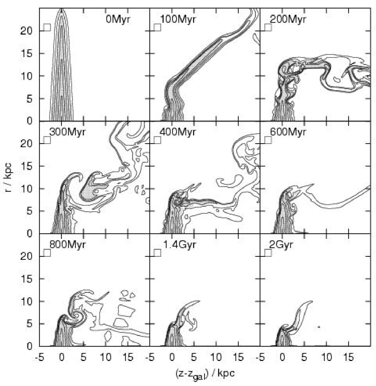
Figure 11: Evolution of gas density distribution for the massive galaxy in a wind with $T_{\mathrm{ICM}}{}_{1}$, $\tilde{p}_{\mathrm{ram}}=1000\,\textrm{cm}^{-3}\,\textrm{km}^{2}\,\textrm{s}^{-2}$, Mach 0.8, $t_{\mathrm{switch}}=20\,\textrm{Myr}$. The density distribution is shown by contour lines with the inmost contour at $10^{-24}\,\textrm{g}\,\textrm{cm}^{-3}$; the spacing of the contours is half an order of magnitude. Only contours for $\rho>\rho_{\mathrm{ICM}}$ are shown. In the shaded regions the gas is still bound to the galactic potential. The size of the small rectangle in the top left corner corresponds to $10\times 10$ grid cells.

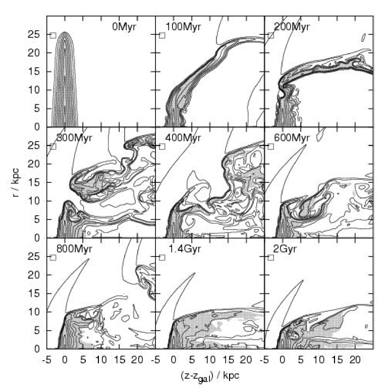
Figure 12: Like Fig. 11, but for a wind with $\tilde{p}_{\mathrm{ram}}=1000\,\textrm{cm}^{-3}\,\textrm{km}^{2}\,\textrm{s}^{-2}$, Mach 2.53. Again contours for $\rho>\rho_{\mathrm{ICM}}$ are shown. Here $\rho_{\mathrm{ICM}}$ is lower than in Fig. 11, hence there are more contour lines in this plot. As this is a supersonic wind, also a bow shock appears.

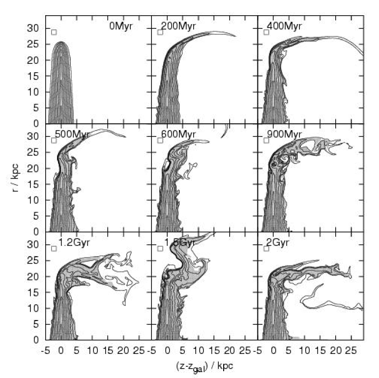
Figure 13: Like Fig. 11, but for a weak wind with $\tilde{p}_{\mathrm{ram}}=10\,\textrm{cm}^{-3}\,\textrm{km}^{2}\,\textrm{s}^{-2}$, Mach 0.8. Concerning the number of contour lines, see the comment at Fig. 12.

We find that the ICM-ISM stripping proceeds in three phases:

Instantaneous stripping:

First the outer gas disk, down to a certain radius, is bent towards the downstream side of the galaxy. This phase can be seen in the first panel with $t>0\,\textrm{Myr}$ in Figs. 11 to 13. The time scale on which the bending takes place is determined by the ram pressure. It reaches from a few $10\,\textrm{Myr}$ for high ram pressures to about $200\,\textrm{Myr}$ for low ram pressures. Also the radius down to which the disk is bent depends on the strength of the ram pressure. Reasonably, for higher ram pressures only a small inner part is retained, and for low ram pressures only the outer edge is bent, but the disk is affected even for very small ram pressures. In all cases a large part of the matter that is pushed out of its original position is still bound.

Intermediate phase:

The first phase is followed by a quite dynamical intermediate phase, during which the bent-out part of the disk breaks up. A part of the material that is pushed out is now stripped completely and a part falls back to the original disk region. This back-fall always happens in the lee of the galaxy, where the displaced gas is protected against the wind. This phase in which bound gas can be found behind the gas disk was also noticed by Schulz & Struck (2001). The duration of this phase depends on the ram pressure. For high ram pressures it is short (a few $100\,\textrm{Myr}$), for low ram pressures this phase continues for the rest of the simulation (up to $2\,\textrm{Gyr}$).

Continuous stripping:

Actually the continuous stripping –the peeling off of the outer disk layers of the upstream side of the gas disk by the Kelvin-Helmholtz (KH) instability – works on the gas disk from the beginning on. However, the effect of this process is quite small, so that it is not distinct before the first two phases are finished. This status is only reached for stronger ram pressures, as for weaker ones the intermediate phase is long. Even though the effect of the continuous stripping is small, it slowly decreases the mass and the radius of the remaining gas disk.

Typical for the supersonic runs is a stagnant region in the wake of the galaxy, where gas with low densities, that is still bound to the galaxy, tends to linger (see final stages in Fig. 12).

In all runs bound gas can be found at quite large distances (10 to $15\,\,\textrm{kpc}$) behind the galaxy during the instantaneous stripping phase and the intermediate dynamic phase. For lower ram pressures some gas packages are still bound at distances of $20\,\,\textrm{kpc}$ behind the galaxy.

Another feature that appears in all simulations is the flittering of the outer edge of the galaxy. The KH-instability pulls low density tongues along the upstream side of the remaining gas disk from the centre towards the edge. There these pieces of gas are exposed to the full wind and blown away (see e.g. last two panels in Fig. 11). This procedure repeats continuously and leads to an oscillation in the radius of the gas disk $r_{\mathrm{disk}}(t)$.

The evolution of the density in the galactic plane and the surface density profile are shown in Fig. 14 for a stronger and for a weak subsonic wind.

Figure 14: Evolution of density $\rho$ and surface density $\Sigma$ profiles along the galactic plane for to the runs shown in Figs. 11 (left) and 13 (right). For the calculation of $\Sigma$ we integrate over interval $(z_{\mathrm{gal}}-5\!\,\textrm{kpc},z_{\mathrm{gal}}+5\!\,\textrm{kpc})$ to avoid that stripped material at larger distances to the galaxy appears in $\Sigma$.

As long as a substantial part of the gas disk remains, neither the density profile nor the surface density in the inner part change much. However, we observe a compression of the outer layers on the upstream side of the gas disk (see Sect. 5.5). For low ram pressures only the very outer layers are compressed, for stronger winds the compression goes deeper towards the galactic plane.

5.3 Varying the wind parameters

In this Sect. we show how the results for the gas disk radius $r_{\mathrm{disk}}(t)$, the gas mass inside the original disk region $M_{\mathrm{orig}}(t)$ and the bound gas mass $M_{\mathrm{bnd}}(t)$ depend on the wind strength. We also show in separate plots (in order to maintain clarity) how much bound gas can be found outside the original disk region (that is $M_{\mathrm{bnd}}(t)-M_{\mathrm{orig}}(t)$) and how much fallen back gas is contained inside the original disk region (this is $M_{\mathrm{fb}}(t)$, see Sect. 4.5.1). We scan the wind parameter space for three different cases:

• The massive galaxy in different ICM winds with ICM temperature $T_{\mathrm{ICM}}{}_{1}$ (corresponding to an ICM sound speed of $1000\,\textrm{km}\,\textrm{s}^{-1}$).

• The massive galaxy in different ICM winds with ICM temperature $T_{\mathrm{ICM}}{}_{2}$ (corresponding to an ICM sound speed of $562\,\textrm{km}\,\textrm{s}^{-1}$).

• The medium galaxy in different ICM winds with ICM temperature $T_{\mathrm{ICM}}{}_{1}$ (corresponding to an ICM sound speed of $1000\,\textrm{km}\,\textrm{s}^{-1}$).

As a representative case, the results of case (a) are shown in Figs. 15, 16 and 17. Corresponding plots for cases (a) and (b) are very similar.

Figure 15: Gas disk radius $r_{\mathrm{disk}}(t)$ (top panel), mass $M_{\mathrm{orig}}(t)$ in the original disk region (middle panel) and bound gas mass $M_{\mathrm{bnd}}(t)$ (bottom panel) of the massive galaxy in ICM winds with $T_{\mathrm{ICM}}{}_{1}$ for different ram pressures $\tilde{p}_{\mathrm{ram}}$ and Mach numbers. Curves for the same $\tilde{p}_{\mathrm{ram}}$ group together. Each group is labelled accordingly with its $\tilde{p}_{\mathrm{ram}}$ in units of $\,\textrm{cm}^{-3}\,\textrm{km}^{2}\,\textrm{s}^{-2}$. The Mach number of each curve is coded by the line style, see key in the middle panel. The right axes are labelled in units of the initial radius or mass.
In the top panel all curves except the ones for Mach 0.8 are shown in the smoothed version (see text) for clarity. The frequency and amplitude in $r_{\mathrm{disk}}(t)$ are comparable for all runs with the same $\tilde{p}_{\mathrm{ram}}$.
The vertical bars show where we consider the intermediate phase to be finished. The two thin vertical lines mark the moment when the flow reaches the galaxy ($t_{0}=40\,\textrm{Myr}$) and $t_{0}+t_{\mathrm{switch}}=60\,\textrm{Myr}$.

Figure 16: Mass of bound gas outside the original disk region as a function of time; for the massive galaxy in different ICM winds ($T_{\mathrm{ICM}}{}$). There is one labelled panel for each ram pressure. Inside the panels the Mach numbers of the wind is coded by the line style (see key). The right axes are labelled in units of the initial radius or mass.

Figure 17: Mass of fallen back gas $M_{\mathrm{fb}}(t)$(= galactic gas that has left the original disk region and fell back to that region) as function of time; for the massive galaxy in different ICM winds ($T_{\mathrm{ICM}}{}_{1}$). There is one labelled panel for each ram pressure. Inside the panels the Mach numbers of the wind is coded by the line style (see key). The right axes are labelled in units of the initial radius or mass.

For clarification we apply a time-averaging to most $r_{\mathrm{disk}}(t)$ curves, smoothing the oscillations that are due to the flittering edge of the galaxy (see end of Sect. 5.2). We average $r_{\mathrm{disk}}(t)$ over $100\,\textrm{Myr}$ for the cases with $\tilde{p}_{\mathrm{ram}}\geq 1000\,\textrm{cm}^{-3}\,\textrm{km}^{2}\,\textrm{s}^{-2}$ ($\tilde{p}_{\mathrm{ram}}\geq 100\,\textrm{cm}^{-3}\,\textrm{km}^{2}\,\textrm{s}^{-2}$ for the medium galaxy) and over $200\,\textrm{Myr}$ for the lower ram pressure cases. The smoothing is applied neither to the initial $250\,\textrm{Myr}$ ($500\,\textrm{Myr}$) for the stronger ram pressures (for the weaker ram pressures), nor to the curves for $\tilde{p}_{\mathrm{ram}}=10\,\textrm{cm}^{-3}\,\textrm{km}^{2}\,\textrm{s}^{-2}$. Also in each group of constant ram pressure we leave one curve oscillating. The amplitude and the frequency of the oscillations are similar within a group.

The first thing to notice is that the mass and radius of the remaining gas disk depend mainly on the ram pressure with higher ram pressures resulting in smaller disks. For the strongest ram pressures even the complete gas disk is stripped. At second glance one can see that for a given ram pressure the gas loss is stronger for subsonic winds than for supersonic ones.

The phases of the stripping process as they were explained in Sect. 5.2 are clearly visible in the $r_{\mathrm{disk}}(t)$, $M_{\mathrm{orig}}(t)$ and $M_{\mathrm{bnd}}(t)$ curves. The bending of the outer gas disk during the instantaneous stripping phase results in a first strong decrease of $r_{\mathrm{disk}}(t)$ and $M_{\mathrm{orig}}(t)$. We define the duration of this phase $\tau_{\mathrm{push}}$ to last from the moment the flow reaches the galaxy to the first local minimum in $r_{\mathrm{disk}}(t)$. Fig. 27 shows the dependence of $\tau_{\mathrm{push}}$ on ram pressure, this point is discussed in Sect. 5.7.1. After the instantaneous stripping phase, the intermediate dynamic phase follows with the falling back of some gas. This can be seen in the slight increase of $M_{\mathrm{orig}}(t)$ just after the initial decrease, and of course in the plot showing $M_{\mathrm{fb}}(t)$ directly (Fig. 17). Although the gas disk always reacts to the wind in the initial instantaneous stripping phase, only for stronger winds this also results in unbinding a substantial amount of gas from the galactic potential. The duration of the intermediate phase, this is until most of the bound gas outside the disk region has vanished, takes much longer for weak winds than for strong ones. For ram pressures of $10\,\textrm{cm}^{-3}\,\textrm{km}^{2}\,\textrm{s}^{-2}$ this phase is not finished at the end of the simulations. For all but the very weakest ram pressure, during the first few $100\,\textrm{Myr}$ between 20 and 40% of the original gas disk mass linger outside the original disk region but are still bound. The amount of gas that falls back to the original disk region is of the order of 5 to 10% of the original gas disk mass.

For the weakest ram pressure ($\tilde{p}_{\mathrm{ram}}=10\,\textrm{cm}^{-3}\,\textrm{km}^{2}\,\textrm{s}^{-2}$) the galaxy loses only a few percent of its gas, although also in this case the radius of the gas disk is truncated.

5.4 Influence of the wind initialisation

We test how our results are influenced by the initialisation of the simulations (see Sect. 4.2). In addition to the standard case $t_{\mathrm{switch}}=20\,\textrm{Myr}$ we rerun a few representative cases with $t_{\mathrm{switch}}=70\,\textrm{Myr}$ and $t_{\mathrm{switch}}=150\,\textrm{Myr}$. The resulting mass and radius of the gas disk for two of these winds are shown in Fig. 18.

Figure 18: Comparison of stripping radius $r_{\mathrm{disk}}(t)$, mass in original disk region $M_{\mathrm{orig}}(t)$ and bound mass $M_{\mathrm{bnd}}(t)$ for different $t_{\mathrm{switch}}$, for two representative winds. We marked the moment where a sound wave starting at the inflow boundary reached galaxy ($t_{0}$), and $t_{0}+t_{\mathrm{switch}}$ for the three different $t_{\mathrm{switch}}$ by the four thin vertical lines. For further explanations see Fig. 15.

Again we smooth the curves for $r_{\mathrm{disk}}(t)$ (see Sect. 5.3). Different $t_{\mathrm{switch}}$ result in expected systematic differences during the initial phase. The decrease in mass and radius due to the instantaneous stripping is fastest for the shortest $t_{\mathrm{switch}}$. After that $r_{\mathrm{disk}}$, $M_{\mathrm{orig}}$ and $M_{\mathrm{bnd}}$ agree well despite the different $t_{\mathrm{switch}}$. The cases with the longest $t_{\mathrm{switch}}$ tend to retain a little more mass during the intermediate phase. For weaker $\tilde{p}_{\mathrm{ram}}$ the agreement between cases with different $t_{\mathrm{switch}}$ is not as tight as for strong $\tilde{p}_{\mathrm{ram}}$, which is due to the longer dynamic (chaotic) intermediate phase for weaker $\tilde{p}_{\mathrm{ram}}$. The qualitative behaviour of the amount of bound mass outside the disk region and of the fallen back mass is independent of $t_{\mathrm{switch}}$.

5.5 Influence of the vertical structure of the gas disk

In order to study the influence of the vertical structure of the gas disk we perform some simulation runs with exponential and flared disks of varying scale heights in representative wind cases (see Table 3). Fig. 19 shows snapshots at the same moment during the instantaneous stripping phase for three exponential disks with different scale heights.

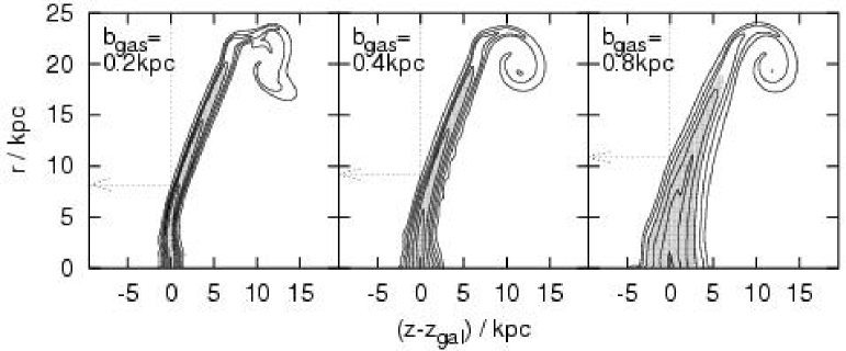
Figure 19: Density contours at 70Myr for three different gas disk thicknesses ($b_{\mathrm{gas}}=0.2,0.4,0.8\,\textrm{kpc}$). Gas in the shaded region is bound to the galactic potential. The wind was the same in all cases ($\tilde{p}_{\mathrm{ram}}=1000\,\textrm{cm}^{-3}\,\textrm{km}^{2}\,\textrm{s}^{-2}$, $T_{\mathrm{ICM}}{}_{1}$, Mach 0.8). The method of radius measurement is illustrated (see Sect. 4.5.1).

Despite their different thickness, all three cases look very similar. The resulting radius and mass curves are compared in Fig. 20 for two of the winds.

Figure 20: Comparison of stripping radius $r_{\mathrm{disk}}(t)$, mass in original disk region $M_{\mathrm{orig}}(t)$ and bound mass $M_{\mathrm{bnd}}(t)$ for different vertical structures, for two representative winds. For further explanations see Fig. 15. All radius curves are smoothed as explained in Sect. 5.3.

It does not make sense to use $M_{\mathrm{orig}}$ for this comparison, as for gas disks with different thicknesses and shapes also the original disk regions differ strongly. Hence we use $M_{\mathrm{cyl}}$ here, the mass inside the cylinder with $r<26\,\textrm{kpc}$ and $|z-z_{\mathrm{gal}}|<5\,\textrm{kpc}$. The different starting points of the curves for the bound mass are due to the different disk thicknesses and external pressures (see Sect. 3.2.4 and Fig. 6); for thicker disks the outer layers become unbound. The radius curves are again smoothed as explained in Sect. 5.3.

The $r_{\mathrm{disk}}$ as well as $M_{\mathrm{cyl}}$ and $M_{\mathrm{bnd}}$ are nearly independent of the vertical structure of the gas disk. For the higher ram pressure of $1000\,\textrm{cm}^{-3}\,\textrm{km}^{2}\,\textrm{s}^{-2}$ the results for the different gas disks agree excellently. For the lower ram pressure ($100\,\textrm{cm}^{-3}\,\textrm{km}^{2}\,\textrm{s}^{-2}$) the scatter is a bit larger as the galaxies stay longer in the dynamic intermediate phase. The difference in the radius curves during the initial instantaneous stripping phase are due to the method of measurement, as is demonstrated in Fig. 19. We conclude from this test that the success of RPS is independent of the vertical structure of the gas disk.

We compare the compression of the upstream side of the gas disk for different scale heights and winds by showing the evolution of the vertical density profile through the gas disk at $r=0.23\,\textrm{kpc}$ in Fig. 21.

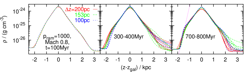
Figure 21: Evolution of vertical profiles at $r=0.23\,\textrm{kpc}$ for different winds and gas disk thickness. We used an exponential disk for all cases, the scale heights were $b_{\mathrm{gas}}=0.2\,\textrm{kpc}$ (thin), $b_{\mathrm{gas}}=0.4\,\textrm{kpc}$ (standard) and $b_{\mathrm{gas}}=0.8\,\textrm{kpc}$ (thick). We fitted an exponential function to the steepened part of the profile, the scale height for this fit was approximately $0.12\,\textrm{kpc}$ for all cases. In the bottom line the variation of the vertical profiles with resolution for three different time steps/time intervals is demonstrated (colour version in online paper).

The compression of the upstream side of the gas disk results in a steepening of the density profile of the outer layers. In the compressed region the density profile can be fitted with an exponential function of a smaller scale height than the original $b_{\mathrm{gas}}$. The scale height in the compressed layers is about $0.12\,\textrm{kpc}$ independently of the wind and the original $b_{\mathrm{gas}}$, but for stronger ram pressures the compressed layer reaches deeper towards the galactic plane. The dependence of the scale height of the compressed layer on resolution is demonstrated in the bottom line in Fig. 21, it is only a weak dependence. This plot shows vertical profiles at $t=100\,\textrm{Myr}$ and in the time intervals $300$-$400\,\textrm{Myr}$ and $700$-$800\,\textrm{Myr}$. We chose to show time intervals to allow averaging over the intrinsic oscillations in the profiles. In any way, if the scale height of the compressed layer was set by the resolution, it should vary from thick to thin disks. For the medium galaxy the profile of the outer layers is steepened to a scale height of about 0.09kpc.

5.6 Cross-comparisons between runs with different $T_{\mathrm{ICM}}$

The results from Sect. 5.3 suggest that the effect of the stripping does not depend on the ram pressure alone but also slightly on the Mach number. To investigate this point further we compare runs with different ICM temperatures. E.g. for $T_{\mathrm{ICM}}{}_{1}$ the velocity of $800\,\textrm{km}\,\textrm{s}^{-1}$ is equivalent to Mach number 0.8, whereas for $T_{\mathrm{ICM}}{}_{2}$ the same velocity corresponds to Mach number 1.423. The velocity that belongs to Mach number 0.8 for $T_{\mathrm{ICM}}{}_{2}$ is $450\,\textrm{km}\,\textrm{s}^{-1}$. If indeed the Mach number is the determining parameter, then for this example the result of the run with $(T_{\mathrm{ICM}}{}_{1},800\,\textrm{km}\,\textrm{s}^{-1},\textrm{Mach number}\,0.8)$ should be the same as the result of the case $(T_{\mathrm{ICM}}{}_{2},450\,\textrm{km}\,\textrm{s}^{-1},\textrm{Mach number}\,0.8)$ rather than $(T_{\mathrm{ICM}}{}_{2},800\,\textrm{km}\,\textrm{s}^{-1},\textrm{Mach number}\,1.423)$. We show this comparison for $r_{\mathrm{disk}}(t)$, $M_{\mathrm{orig}}(t)$ and $M_{\mathrm{bnd}}(t)$ in Fig. 22 for some cases.

Figure 22: Comparison of stripping radius $r_{\mathrm{disk}}(t)$, mass in original disk region $M_{\mathrm{orig}}(t)$ and bound mass $M_{\mathrm{bnd}}(t)$ for selected runs with $\tilde{p}_{\mathrm{ram}}=1000\,\textrm{cm}^{-3}\,\textrm{km}^{2}\,\textrm{s}^{-2}$ (upper panel) and $\tilde{p}_{\mathrm{ram}}100=\,\textrm{cm}^{-3}\,\textrm{km}^{2}\,\textrm{s}^{-2}$ (lower panel). For further explanations see Fig. 15. See also Sect. 5.6.

In the middle panel, where the velocity is subsonic for $T_{\mathrm{ICM}}{}_{1}$ and supersonic for $T_{\mathrm{ICM}}{}_{2}$, indeed runs with the same Mach number rather than with the same velocity correspond to each other. The same seems to hold for the left panels, in the pure subsonic range, although not as clear as in the transition from the subsonic to the supersonic regime. In the supersonic range (right panels) no systematic difference is seen. As qualitative issues we conclude that (i) for a given wind density and velocity, RPS is slightly more effective if this wind is subsonic (compared to supersonic winds); and (ii) that in the subsonic regime winds with smaller Mach numbers are a bit more effective than winds with higher Mach numbers. Nevertheless, the Mach number is only a secondary parameter, the main parameter is the ram pressure.

Moreover, we do not want to over-interpret the differences between the subsonic and supersonic cases, as we used a single-fluid description. In contrast, the ICM is highly ionised and actually consists of a proton and an electron fluid. With respect to the proton fluid, the galaxy’s velocities are transonic, but with respect to the electron fluid they still move subsonically. Portnoy et al. (1993) studied the difference between the single-fluid and a two-fluid description for a spherical galaxy (with gas replenishment) and found no difference for the amount of gas remaining inside the galaxy.

5.7 Comparison of analytical estimate and numerical result

5.7.1 Instantaneous stripping

We have found that during the instantaneous stripping phase the outer part of the gas disk is displaced, but not immediately unbound. It takes a while until the displaced gas is also unbound. As the analytical estimate in Eq. 1 just compares the forces working on the gas disk, it tells how much gas will be unbound, but it cannot quantify how long this process may take. As the analytical estimate states how much gas will be unbound from the galaxy, we also need to extract this quantity from the simulations. Hence we measure the radius and the mass of the remaining gas disk at the end of the dynamic intermediate phase, i.e. when no substantial amount of bound gas outside the disk region is left. We have marked this moment in Fig. 15 by vertical bars. For the lowest ram pressure ($\tilde{p}_{\mathrm{ram}}=10\,\textrm{cm}^{-3}\,\textrm{km}^{2}\,\textrm{s}^{-2}$) the intermediate phase is not completed during the simulation run time, here we use the final values for the comparison.

As we pointed out in Sect. 5.1.1, there are several versions how the analytical estimate can be done, therefore we discuss the following recipes:

• Use Eq. 14 to compute the restoring force while using the maximal potential gradient inside the original disk region (marked by “$\Sigma/$in disk” in Figs. 23 and 24).

• Use Eq. 15 with $\Delta z=150\,\textrm{pc}$ and use the maximal potential gradient inside the original disk region (marked by “$\rho/$in disk” in Figs. 23 and 24).

• Use Eq. 15 with $\Delta z=150\,\textrm{pc}$ and use the maximal potential gradient found for any $z$ (marked by “$\rho/$ all $z$” in Figs. 23 and 24).

• Compare the thermal pressure in the galactic plane and the ram pressure (Eq. 16, marked by “pressures” in Figs. 23 and 24)

Version (c) is between (a) and (b); for higher ram pressures it is indistinguishable from version (b), as there smaller radii are concerned where the steepest potential gradient is found inside the disk region. Also the result from the pressure comparison (d) has a very similar shape to (a) and (b) and is between those two. As already mentioned in Sect. 5.1.1, the estimates according to versions (a) and (b) are identical despite a shift in horizontal direction for exponential disks. These two versions represent the two extremes in the uncertainty how the gravitational restoring force $f_{\mathrm{grav}}$ shall be computed – either simplifying to a thin disk (a) or computing $f_{\mathrm{grav}}$ for a single cell only (b). This uncertainty can be parametrised by a factor of $\alpha$ in the calculation of $f_{\mathrm{grav}}$, modifying Eq. 14 to

$$|f_{\mathrm{grav}}(z,r)|=\alpha\left|\frac{\partial\Phi}{\partial z}(z,r)\Sigma_{\mathrm{gas}}(r)\right|.$$ (27)

Choosing $\alpha=1$ corresponds to version (a), choosing $\alpha=0.16$ recovers version (b), but $\alpha$ can be adjusted to fit the numerical results.

Before we do any fitting, we show the pure analytical estimates (versions (a) to (d)) and the numerical results in Fig. 23 for the massive galaxy and in Fig. 24 for the medium galaxy.

Figure 23: Comparison of analytical estimate and numerical result for the stripping radius and the remaining gas mass as a function of ram pressure, for the massive galaxy. We show four versions of the analytical estimate, see Sect. 5.7.1. The Mach numbers for the numerical result are coded with different symbol shapes. Open symbols are for cases with $T_{\mathrm{ICM}}{}_{1}$, solid symbols of the same shape for cases with $T_{\mathrm{ICM}}{}_{2}$.

Figure 24: Same as Fig. 23, but for the medium galaxy.

The numerical results are indeed in the range suggested by the analytical estimates.

We also want to consider the Mach number dependence of the numerical results again. So far we calculated the ram pressure according to $\tilde{p}_{\mathrm{ram}}=n_{\mathrm{ICM}}v_{\mathrm{ICM}}^{2}$ for the supersonic cases as well. However, the velocity and density behind the formed bow shock differ from the values on its upstream side. It may be more appropriate to calculate the ram pressure for supersonic winds with the values of $\rho$ and $v$ at the downstream side of a straight shock with the corresponding Mach number. The component of the momentum density $\rho_{\mathrm{ICM}}v_{\mathrm{ICM}}$ perpendicular to the shock front is conserved across such a shock, whereas the velocity at the downstream side is reduced (and the density increased) by a certain factor according to the Rankine-Hugoniot conditions. Then also the true ram pressure would be diminished by the same factor as $v$. For Mach numbers of 1.423 and 2.53 (at the upstream side) the velocity at the downstream side is reduced by factors of 0.62 and 0.36, respectively. In Figs. 25 and 26 we replot the numerical results with this correction, that is shifting the points for the supersonic results down to the corrected ram pressures.

Figure 25: Comparison between the analytical estimates and the numerical result for the massive galaxy with Rankine-Hugoniot-corrected ram pressures for the supersonic cases (see text). Open and solid symbols are for cases with $T_{\mathrm{ICM}}{}_{1}$ and $T_{\mathrm{ICM}}{}_{2}$, respectively. The symbol shape codes the Mach number. The analytical estimate for the force comparison (solid line) is fitted to the numerical results via the parameter $\alpha$ (see also text). The estimate from the pressure comparison is repeated unmodified.

Figure 26: Same as Fig. 25, but for the medium galaxy.

In addition, we repeat the analytical estimate from the pressure comparison (version (d), marked with “pressures” in Figs. 25 and 26) and plot the estimate from the force comparison with an adjusted $\alpha$ (see Eq. 27, marked with “forces, $\alpha=0.25$” in Figs. 25 and 26). For $\alpha=0.25$ the numerical result and the analytical estimate agree well. In contrast to the uncertainty expressed by $\alpha$ in the force comparison, there is no uncertainty in the pressure comparison. And indeed the (Rankine-Hugoniot-corrected) numerical result and the estimate from the pressure comparison are in good agreement. With $\alpha=0.25$, the estimate from the force comparison was shifted to match the result from the pressure comparison. The point for the lowest ram pressure and Mach 2.53 in Fig. 26 that lies above the analytical estimate is explained easily because the dynamic intermediate phase for this run is not finished at the end of the simulation. We note that the correction of the ram pressures for the supersonic cases according to the Rankine-Hugoniot conditions cannot describe the situation completely, because it would mean that also in the supersonic range the results should depend slightly on the Mach number. This is not found in the simulations (see Sect. 5.6).

We can also compare the predicted duration for the instantaneous stripping with the numerical result. The prediction drawn from Eq. 22 refers only to the replacement of the outer gas disk. The numerical result for the replacement is given by the time of the first local minimum in the $r_{\mathrm{disk}}$ curves in Fig. 15. The trends in the numerical result and the analytical estimate shown in Fig. 27 agree well, also the absolute values agree roughly.

Figure 27: Duration of the instantaneous stripping phase and intermediate phase as a function of ram pressure. Large symbols are for the massive galaxy, small symbols for medium galaxy. Also the analytical estimate for the instantaneous phase according to Eq. 22 is shown, the solid line is for the massive galaxy, the dashed one for the medium galaxy.

We also show the duration of the intermediate phase, that is the time until all gas that is not bound tightly enough is truly unbound. We find that this time is approximately 10 times as long as the instantaneous stripping phase.

5.7.2 Continuous stripping

The estimate of the mass loss rate during the continuous stripping phase (see Sect. 5.1.2) is only a rough one. The mass-loss rates are expected to be of the order of one $M_{\sun}\,\,\textrm{yr}^{-1}$. Fig. 28 demonstrates the mass-loss rates derived from the simulations by fitting a linear function to $M_{\mathrm{bnd}}(t)$ during the continuous stripping phase.

Figure 28: Mass loss rates of the continuous stripping phase as a function of ram pressure. The Mach numbers are coded by different symbols. Symbols of group (I) (large symbols) are for the massive galaxy in winds with $T_{\mathrm{ICM}}{}_{1}$, group (II) (medium-size symbols) for the massive galaxy in winds with $T_{\mathrm{ICM}}{}_{2}$, and group (III) (small symbols) for the medium galaxy in winds with $T_{\mathrm{ICM}}{}_{1}$. We also show the rough analytical estimate (see Eq. 25 in Sect. 5.1.2).

Because the runs with $\tilde{p}_{\mathrm{ram}}=10\,\textrm{cm}^{-3}\,\textrm{km}^{2}\,\textrm{s}^{-2}$ do not reach the continuous phase during the runtime, for those runs we fit the time range between 1 and $2\,\textrm{Gyr}$. From the simulations we can derive mass-loss rates between 0.1 and $2\,M_{\sun}\,\,\textrm{yr}^{-1}$. Except that the highest ram pressures produced the highest mass-loss rates, we cannot find any further trends. The analytical estimate could give a rough impression only.

6 Discussion and conclusions

6.1 Influence of the ICM pressure

What happens to the gas disk of a spiral galaxy in a high pressure external medium? From the comparison of typical pressures in the disks of isolated galaxies ($10^{-13}$ to $10^{-11}\,\textrm{erg}\,\,\textrm{cm}^{-3}$) and typical ICM pressures (e.g. $1.4\cdot 10^{-13}\,\textrm{erg}\,\,\textrm{cm}^{-3}$ for $n_{\mathrm{ICM}}=10^{-4}\,\textrm{cm}^{-3}$ and $T_{\mathrm{ICM}}=10^{7}\,\textrm{K}$) alone it is obvious that normal disk galaxies cannot exist in cluster environments, no matter if they move or not. If for an isolated galaxy the external pressure is increased gradually, the disk has two alternatives to react to that. Either, if the density distribution should not change much, it has to heat up in order to reach higher pressures so that it can maintain pressure equilibrium with the surrounding gas. This is what we assumed implicitly with our initial conditions. Or, if cooling prohibits a substantial increase of the temperature, the disk will be compressed. However, this is only the crude basic idea. The fate of a more realistic multi-phase gas disk including effects like star formation and feedback may be much more complicated. Due to the compression the formation of molecular clouds and stars may be enhanced, which in turn could increase the amount of heating by an increased supernova rate and stellar winds. The observational fact that even HI-deficient cluster galaxies contain a rather normal amount of molecular gas (Kenney & Young 1989; Boselli et al. 1997; Casoli et al. 1998) and show normal to enhanced star formation rates in their inner part (Koopmann & Kenney 1998, 2004a, 2004b) supports this picture. It would be worth to study the effect of the external pressure on the gas disks of spiral galaxies in a separate work.

In how far does our setup of the initial model (fixing the density distribution of the gas disk and calculating the temperature distribution from hydrostatic equilibrium), which leads to high disk temperatures, bias the results derived in this paper? The concern is that due to the high temperature (and hence higher thermal energy) our gas disks are not bound as strongly as cooler disks in isolated galaxies and hence are stripped easier. In this case we would overestimate the stripping efficiency. The alternative way of initial setup would be to fix the temperature inside the gas disk (e.g. determined by the heating-cooling balance) as well as its mass and calculate the density distribution from the hydrostatic equation. The resulting gas disks would become thinner and have higher densities as the external ICM pressure increases. In varying the gas disk thickness and shape (see Sect. 5.5) we have already checked if such thin disks are harder to strip by ram pressure, but we did not find them to be more resistant to RPS. We also performed test runs that started with a galaxy resembling an isolated one (concerning disk pressure and temperature), but put into a high-pressure ICM. As this galaxy was not in hydrostatic equilibrium with the ICM, it was compressed immediately and then stripped like its equilibrium analogue. Hence we conclude that our results are not biased strongly by the initial pressure and temperature distribution.

6.2 Morphological features of stripped galaxies

In agreement with previous work, our simulations suggest that disk galaxies suffering (approximately) face-on RPS should have truncated disks, where the radius of the disk is set by the ram pressure and the galactic potential. Moreover, if they are in the instantaneous stripping phase or the dynamic intermediate phase, stripped gas could be found at distances as far as $20\,\textrm{kpc}$ behind the disk. How long such structures exist depends at least on $\tilde{p}_{\mathrm{ram}}$. In how far this stripped gas actually remains visible, is dispersed or cools, forms stars or is affected by heat conduction, our simulations cannot predict as they do not include such processes. Due to the homogeneous gas disk used in our simulations, filaments emerging from the disk are found mainly at the disk edge. Such examples are indeed observed (e.g. NGC 4522: Vollmer et al. (2004b) and references therein, NGC 4402: Cayatte et al. (1990, 1994); Crowl et al. (2004)). The filaments found in NGC 4569 (Tschöke et al. 2001; Vollmer et al. 2004a; Kenney et al. 2004; Bomans et al. 2004) seem not to emerge from the edge but more from the centre of the disk. This may be due to activity in the galactic nucleus or due to RPS of an inhomogeneous gas disk.

6.3 Mixing with the ICM

We tried to infer to what extend ICM gets mixed into the remaining gas disk. Such mixing would change the angular momentum and metalicity of the gas disk. To investigate this point we used two more recipes to compute the mass of the gas disk or the bound mass. In contrast to summing over the “coloured” gas (the gas that has been inside the galactic disk initially) in the disk region, we also summed up all gas in the disk region with a temperature below $5\cdot 10^{6}\,\textrm{K}$ (about the virial temperature of the massive galaxy). This prevents that we include the ICM that is streaming freely through the already swept disk region, but it would include all ICM that has already mixed with the gas disk. On the other hand, we sum over all gas in the region of the bound gas instead of summing only over the “coloured” gas there. This includes all ICM that is situated in this regions. We find, however, no differences between the versions that should include or exclude the ICM, so we conclude that no ICM is accreted by the galaxy.

6.4 Time dependent winds

During its passage through a cluster a galaxy does not experience a constant wind. Galaxies on more radial orbits fly through the high density cluster core. With a typical velocity of $1000\,\textrm{km}\,\textrm{s}^{-1}$ a galaxy needs $1\,\textrm{Gyr}$ to cross the inner Mpc of the cluster. Vollmer et al. (2001b) calculated the time dependent ram pressure for a galaxy falling into the Virgo cluster (their Fig. 3) and found that typically the ram pressure exceeds $1000\,\textrm{cm}^{-3}\,\textrm{km}^{2}\,\textrm{s}^{-2}$ for about $100\,\textrm{Myr}$ before and after the core passage, and still exceeds $300\,\textrm{cm}^{-3}\,\textrm{km}^{2}\,\textrm{s}^{-2}$ about $250\,\textrm{Myr}$ before and after the core passage. According to our simulations these times are definitely long enough to truncate the radius of the gas disks. However, the duration of the high ram pressure may be too short to unbind all this gas. Even in our simulations with constant winds several $10^{8}M_{\sun}$ fall back to the disk region, and for quite a while about $10^{9}M_{\sun}$ of gas that is still bound lingers behind the galaxy. If the ram pressure abates too early after the core passage all this gas should fall back to the disk. From our simulations we cannot infer in how far and how fast the gas disk resettles after the core passage.

6.5 Galaxies in cluster outskirts and galaxy groups

In our simulations we found that even mild ram pressures of about $100\,\textrm{cm}^{-3}\,\textrm{km}^{2}\,\textrm{s}^{-2}$ and less already truncate the gas disk of massive galaxies to about 15kpc. Even if low ram pressures do not unbind much gas, they still displace the outer parts of the gas disk. The wind itself and back-falling gas disturb the disk, send shock waves through it which could trigger star formation (e.g.  Fujita & Nagashima 1999). We therefore expect that even at larger distances from the cluster centre the gas disks of most galaxies should be “pre-processed” (see also Fujita 2004). This pre-processing of galaxies in cluster outskirts and groups could explain the HI deficient galaxies at large distances to the cluster centre found by Solanes et al. (2001). RPS in low density environments may be more important than thought so far.

6.6 Inclination

We have studied only cases where galaxies move face-on. What can we learn for inclined cases? Marcolini et al. (2003) found that the inclination angle matters only for medium ram pressures. This can be understood also in the context of our simulations. For very weak winds hardly any gas is unbound from the galaxy by the pushing effect, the main mechanism is the continuous stripping. For this mechanism the inclination angle is not important, it works on the whole surface. For very strong winds the complete disk is lost independently of inclination. Only for the intermediate winds the inclination decides how much mass can be pushed out in the beginning, hence for heavily inclined cases less gas is lost in this phase. After that the continuous stripping continues at the stage where the previous phase has ended. Also Quilis et al. (2000) agreed that only strict edge-on galaxies can retain more gas, intermediately inclined galaxies are stripped similarly to face-on ones. This is also in agreement with the results of Vollmer et al. (2001b), who constructed a generalised formula relating the remaining gas mass with the ram pressure and the inclination angle. However, their sticky-particle simulations cannot model the turbulent viscous stripping. Schulz & Struck (2001) found that for inclined galaxies less gas lingers in the lee of the disk, hence our results concerning back-falling gas may change in such situations. However, the unbinding of the gas after it has left the disk region should take some time also for inclined cases.

In addition to the restriction to the face-on case, a 2D code is restricted to rotationally symmetrical cases. However, real systems are not symmetrical, and an asymmetry may change the behaviour of turbulence and instabilities.

6.7 Summary

We performed a large set of numerical simulations of the face-on RPS of disk galaxies in constant ICM winds. We find that even massive galaxies can lose a substantial part of their gas disks, and can be stripped completely in cluster centres. Our simulations also covered low density environments like cluster outskirts, and we find that there galaxies are truncated to 15 to $20\,\textrm{kpc}$. Back-falling gas and the compression from the flow could trigger star formation, hence we expect galaxies to be pre-processed in cluster outskirts and groups as well. Furthermore, the models show that the stripping proceeds in three phases:

• Instantaneous stripping phase: the outer disk is pushed out of its initial position (bent towards the downstream side), but it is only partly unbound. The main radius reduction happens in this phase. This phase is short (20 to $200\,\textrm{Myr}$), its duration as a function of ram pressure can be read from Fig. 27.

• Intermediate phase: rather dynamic, the gas outside the disk region partially falls back to the disk (about 10% of the original gas mass), the rest is completely stripped. This may repeat in cycles. This phase lasts about 10 times as long as the instantaneous stripping phase, it is finished when no substantial amount of bound gas is left outside the disk region. The radius does not change much during this phase, but the bound gas mass and also the gas mass inside the disk region do. The mass and radius of the remaining gas disk at the end of this phase can be predicted best by comparing the thermal pressure in the disk plane and the ram pressure (for details see Sect. 5.1.1, Eq. 16). The analytical estimate and the numerical results for the stripping radius and the remaining gas mass are summarised in Figs. 25 and 26 for the massive and the medium mass galaxy, respectively.

• Quasi-stable continuous stripping: constant small mass loss rate of about $1M_{\sun}\,\,\textrm{yr}^{-1}$, slow decrease of the disk radius.

The main parameter that sets the mass and radius of the remaining gas disk is the ram pressure, but there is a slight dependence on Mach number in the sense that in the subsonic regime and at the transition from the subsonic to the supersonic regime ICM flows of lower Mach numbers result in a bit stronger gas loss than flows with higher Mach numbers. In how far this result holds for a two-fluid treatment of the ICM is unclear.

The mass loss and shrinking of the radius depend only on the surface density of the gas disk, but not on its vertical structure (thickness, flared or exponential).

We observe a compression at the upstream side of the remaining disk, but we do not find an increased surface density.

Appendix A Influence of artificial viscosity

In our simulations we observed the long phase of turbulent viscous stripping. The code uses an artificial viscosity mainly to be able to handle shocks. A concern may be that due to this artificial viscosity the code cannot handle the KH-instability correctly and hence biases the results of the viscous stripping phase. We performed test runs (see Table 4) to investigate the influence of the artificial viscosity by varying the viscosity parameter $C_{2}$ (see Sect. 2).

$\tilde{p}_{\mathrm{ram}}$	Mach number	viscosity parameter
($\,\textrm{cm}^{-3}\,\textrm{km}^{2}\,\textrm{s}^{-2}$)		$C_{2}$ (see Sect. 2)
1000	0.8	1,2,6
$\cdot$	2.53	$\cdot$

Table 4: List of simulations to study the influence of the artificial viscosity. Common parameters for all runs are: massive galaxy with standard exponential disk, ICM wind with $T_{\mathrm{ICM}}{}_{1}$ ($c_{\mathrm{ICM}}=1000\,\textrm{km}\,\textrm{s}^{-1}$).

For the results for the disk radius, mass and bound mass the differences between runs with various viscosities are negligible. We show one case in Fig. 29.

Figure 29: Influence of the viscosity on the evolution of the gas disk radius, mass and fallen-back mass. The value of the viscosity parameter $C_{2}$ (see Sect. 2) is indicated in the key. For further parameters of these runs see Table 4. This plot is for the runs with Mach number 0.8.

Fig. 30 compares snapshots at $t=200\,\textrm{Myr}$ for the test cases with varying viscosity.

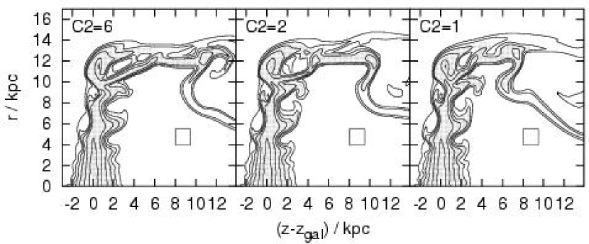
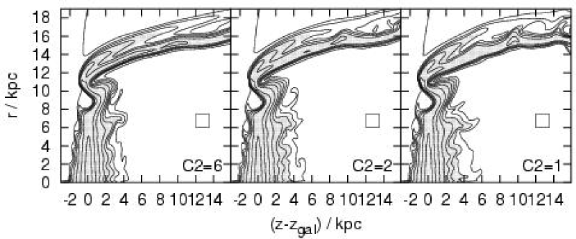
Figure 30: Comparison of the density distribution (at $t=200\,\textrm{Myr}$) for different viscosities. The plot style is the same as in Fig. 11. The top panels are for Mach number 0.8, the bottom panels for Mach number 2.53. For further parameters see Table 4. Each panel is labelled with the appropriate viscosity parameter $C_{2}$ (see Sect. 2). The rectangle corresponds to $10\times 10$ cells.

As expected, for the high viscosity parameter, the surface instabilities are softer, whereas for in the low viscosity case ($C_{2}=1$) the features are sharper. However, almost all features can be identified for all viscosities. We conclude that the use of the artificial viscosity does not bias our results.

Appendix B Influence of resolution

In order to test the influence of the resolution we have performed test runs with resolutions $50\,\textrm{pc}$, $100\,\textrm{pc}$, $150\,\textrm{pc}$ and $200\,\textrm{pc}$.

Fig. 31 compares the radius $r_{\mathrm{disk}}$ and mass $M_{\mathrm{disk}}$ of the remaining gas disk for the standard run (massive galaxy, exponential gas disk, $b_{\mathrm{gas}}=0.4\,\textrm{kpc}$, $t_{\mathrm{ICM}}{}_{1}$, $\tilde{p}_{\mathrm{ram}}=1000\,\textrm{cm}^{-3}\,\textrm{km}^{2}\,\textrm{s}^{-2}$, Mach number 0.8) for the four different resolutions.

Figure 31: Influence of grid size and resolution on evolution of gas disk radius, mass and fallen-back mass. See text for parameters.

Also the the mass of bound gas $M_{\mathrm{bnd}}$ and the mass of fallen-back gas $M_{\mathrm{fb}}$ are shown. The differences for all quantities are negligible. The small differences in $M_{\mathrm{bnd}}$ arise because in cases with higher resolution the the stripped gas can be compressed into smaller volumes, reaching higher densities locally. Such dense clouds are more likely to be bound than the clouds with lower densities.

In Fig. 32 we show snapshots at $t=200\,\textrm{Myr}$ for the four different resolutions.

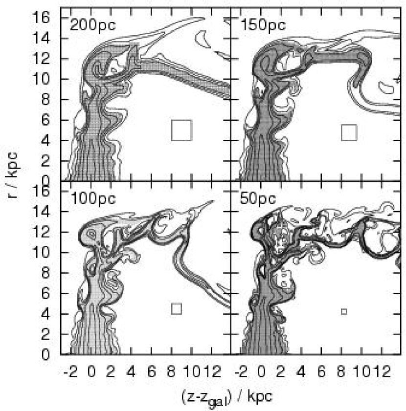
Figure 32: Influence of resolution: Snapshots at $t=200\,\textrm{Myr}$ for four different resolutions as given in the plot, see text for parameters. The plot style is the same as in Fig. 11. The size of $10\times 10$ cells is indicated by the rectangle in each panel.

The strongest difference occurs for the stripped material. The coarser grids cannot resolve the small-scale fragmentation of the stripped gas evident in the highest resolution. However, we did not attempt to interprete the fate of the stripped material shown in the simulations, as we neglected e.g. thermal conduction, which might be play an important role in the evolution of the stripped gas.

References

- Abadi et al. (1999) Abadi, M. G., Moore, B., & Bower, R. G. 1999, MNRAS, 308, 947
- Bomans et al. (2004) Bomans, D. J., Hensler, G., Tschöke, D., Boselli, A., & Napiwotzki, R. 2004, A&A, in press
- Borriello & Salucci (2001) Borriello, A. & Salucci, P. 2001, MNRAS, 323, 285
- Boselli et al. (1997) Boselli, A., Gavazzi, G., Lequeux, J., et al. 1997, A&A, 327, 522
- Burkert (1995) Burkert, A. 1995, ApJ, 447, 25L
- Casoli et al. (1998) Casoli, F., Sauty, S., Gerin, M., et al. 1998, A&A, 331, 451
- Cayatte et al. (1994) Cayatte, V., Kontanyi, C., Balkowski, C., & van Gorkom, J. H. 1994, AJ, 107, 1003
- Cayatte et al. (1990) Cayatte, V., van Gorkom, J. H., & Kotanyi, C. 1990, AJ, 100, 604
- Crowl et al. (2004) Crowl, H. H., Kenney, J. D. P., van Gorkom, J. H., & Vollmer, B. 2004, American Astronomical Society Meeting, 204
- Farouki & Shapiro (1980) Farouki, R. & Shapiro, S. L. 1980, ApJ, 241, 928
- Fujita (2004) Fujita, Y. 2004, PASJ, 56, 29
- Fujita & Nagashima (1999) Fujita, Y. & Nagashima, M. 1999, ApJ, 516, 619
- Gunn & Gott (1972) Gunn, J. E. & Gott, J. R. 1972, ApJ, 176, 1
- Hernquist (1993) Hernquist, L. 1993, ApJS, 86, 389
- Kenney et al. (2004) Kenney, J. D. P., Crowl, H., van Gorkom, J., & Vollmer, B. 2004, in IAU Symposium Series, Vol. 217, Recycling Intergalactic and Interstellar Matter, ed. P. Duc, J. Braine, & E. Brinks (PASP), 370
- Kenney & Koopmann (1999) Kenney, J. D. P. & Koopmann, R. A. 1999, AJ, 117, 181
- Kenney & Koopmann (2001) Kenney, J. D. P. & Koopmann, R. A. 2001, in ASP Conf. Ser., Vol. 240, Gas and Galaxy Evolution, ed. J. E. Hibbard, M. P. Rupen, & J. J. van Gorkom (San Francisco: ASP), 577
- Kenney & Young (1989) Kenney, J. D. P. & Young, J. S. 1989, ApJ, 344, 171
- Koopmann & Kenney (1998) Koopmann, R. A. & Kenney, J. D. P. 1998, ApJ, 497, 75L
- Koopmann & Kenney (2004a) Koopmann, R. A. & Kenney, J. D. P. 2004a, ApJ, in press, astro-ph/0406243
- Koopmann & Kenney (2004b) Koopmann, R. A. & Kenney, J. D. P. 2004b, ApJ, in press, astro-ph/0209547
- Lohmann (2000) Lohmann, F. C. 2000, Master’s thesis, University of Kiel
- Marcolini et al. (2003) Marcolini, A., Brighenti, F., & A.D’Ercole. 2003, MNRAS, 345, 1329
- Mihos (2004) Mihos, J. C. 2004, in Carnegie Observatories Astrophysics Series, Vol. 3, Clusters of Galaxies: Probes of Cosmological Structure and Galaxy Evolution, ed. J. S. Mulchaey, A. Dressler, & A. Oemler (Cambridge: Cambridge Univ. Press), 278
- Mori & Burkert (2000) Mori, M. & Burkert, A. 2000, ApJ, 538, 559
- Norman & Winkler (1986) Norman, M. L. & Winkler, K.-H. A. 1986, in Astrophysical Radiation Hydrodynamics, ed. K.-H. A. Winkler & M. L. Norman, NATO Advanced Research Workshop (Dortrecht: Reidel), 187
- Nulsen (1982) Nulsen, P. E. J. 1982, MNRAS, 198, 1007
- Portnoy et al. (1993) Portnoy, D., Pistinner, S., & Shaviv, G. 1993, ApJS, 86, 95
- Quilis et al. (2000) Quilis, V., Moore, B., & Bower, R. 2000, Science, 288, 1617
- Różyczka (1985) Różyczka, M. 1985, A&A, 143, 59
- Salucci & Burkert (2000) Salucci, P. & Burkert, A. 2000, ApJ, 537, 9L
- Schulz & Struck (2001) Schulz, S. & Struck, C. 2001, MNRAS, 328, 185
- Severing (1995) Severing, I. 1995, Master’s thesis, University of Kiel
- Solanes et al. (2001) Solanes, J. M., Manrique, A., García-Gómez, C., et al. 2001, ApJ, 548, 97
- Stone & Norman (1992) Stone, J. M. & Norman, M. L. 1992, ApJS, 80, 753
- Toyama & Ikeuchi (1980) Toyama, K. & Ikeuchi, S. 1980, Prog. Theo. Phys., 64, 831
- Tschöke et al. (2001) Tschöke, D., Bomans, D. J., Hensler, G., & Junkes, N. 2001, A&A, 380, 40
- Vollmer (2003) Vollmer, B. 2003, A&A, 398, 525
- Vollmer et al. (2004a) Vollmer, B., Balkowski, C., Cayatte, V., van Driel, W., & Huchtmeier, W. 2004a, A&A, 419, 35
- Vollmer et al. (2004b) Vollmer, B., Beck, R., Kenney, J. D. P., & van Gorkom, J. H. 2004b, AJ, 127, 3375
- Vollmer et al. (2001a) Vollmer, B., Braine, J., Balkowski, C., Cayatte, V., & Duschl, W. J. 2001a, A&A, 374, 824
- Vollmer et al. (2001b) Vollmer, B., Cayatte, V., Balkowski, C., & Duschl, W. J. 2001b, ApJ, 561, 708
- Vollmer et al. (1999) Vollmer, B., Cayatte, V., Boselli, A., Balkowski, C., & Duschl, W. J. 1999, A&A, 349, 411
- Vollmer et al. (2000) Vollmer, B., Marcelin, M., Amram, P., et al. 2000, A&A, 364, 532