Madam - a map-making method for CMB experiments

Abstract

We present a new map-making method for CMB measurements. The method is based on the destriping technique, but it also utilizes information about the noise spectrum. The low-frequency component of the instrument noise stream is modelled as a superposition of a set of simple base functions, whose amplitudes are determined by means of maximum-likelihood analysis, involving the covariance matrix of the amplitudes. We present simulation results with $1/f$ noise and show a reduction in the residual noise with respect to ordinary destriping. This study is related to Planck LFI activities.

1 Introduction

Construction of the CMB map from time-ordered data (TOD) is an important part of the data analysis of CMB experiments. Future space missions like Planck present new challenges for the data analysis. The amount of data Planck produces is far larger than that of any earlier experiments.

The destriping technique (Burigana et al. 1997, Delabrouille 1998, Maino et al. 1999, 2002, Keihänen et al. 2004) provides an efficient map-making method for large data sets. The method is non-optimal in accuracy but fast and stable. Other methods have been developed which aim at finding the optimal minimum-variance map for Planck -like data (e.g. Natoli et al. 2001, Doré et al. 2001, Borrill 1999).

In this paper we present a new map-making method for CMB measurements, called MADAM (Map-making through Destriping for Anisotropy Measurements). The method is built on the destriping technique but unlike ordinary destriping, it also utilizes information about the noise spectrum. The aim is to improve the accuracy of the output map as compared to destriping, while still keeping, at least partly, the speed and stability of the destriping method.

The basic idea of the method is the following. The low-frequency component of the instrument noise in the TOD is modelled as a superposition of simple base functions, whose amplitudes are determined by means of maximum-likelihood analysis, involving the covariance matrix of the amplitudes. The covariance matrix is computed from the noise spectrum, assumed to be known.

This paper is organized as follows. In Section 2 we go through the maximum-likelihood analysis that forms the basis of our map-making method. We describe the map-making algorithm in Section 3. In Section 4 we consider the covariance matrix of component amplitudes. Some technical calculations related to this section are presented in Appenxix A. We give results from numerical simulations in Section 5 and present our conclusions in Section 6.

2 Map-making problem

2.1 Maximum-likelihood analysis of the destriping problem

In the following we present a maximum-likelihood analysis on which our map-making method is based. The analysis is similar to that presented in Keihänen (2004), the main difference being, that here we include the covariance of the correlated noise component.

We write the time-ordered data (TOD) stream as

$${\mathbf{y}}=\mathbf{P}{\mathbf{m}}+{\mathbf{n}}^{\prime}.$$ (1)

Here the first term presents the CMB signal and the second term presents noise. Vector ${\mathbf{m}}$ presents the pixelized CMB map and pointing matrix $\mathbf{P}$ spreads it into TOD.

We divide the noise contribution into a correlated noise component and white noise, and model the correlated part as a linear combination of some orthogonal base functions,

$${\mathbf{n}}^{\prime}=\mathbf{F}{\mathbf{a}}+{\mathbf{n}}.$$ (2)

Vector ${\mathbf{a}}$ contains the unknown amplitudes of the base functions and matrix $\mathbf{F}$ spreads them into TOD. Each column of matrix $\mathbf{F}$ contains the values of the corresponding base function along the TOD. Assuming that the white noise component and the correlated noise component are independent, the total noise covariance is given by

$$\mathbf{C}_{t}=\langle{\mathbf{n}}^{\prime}({\mathbf{n}}^{\prime})^{T}\rangle=\mathbf{F}\mathbf{C}_{a}\mathbf{F}^{T}+\mathbf{C}_{n}$$ (3)

where $\mathbf{C}_{n}=\langle{\mathbf{n}}{\mathbf{n}}^{T}\rangle$ is the white noise covariance, $\mathbf{C}_{a}=\langle{\mathbf{a}}{\mathbf{a}}^{T}\rangle$ is the covariance matrix for the component amplitudes ${\mathbf{a}}$, and $\langle x\rangle$ denotes the expectation value of quantity $x$.

Our aim is to find the maximum-likelihood estimate of ${\mathbf{m}}$ and ${\mathbf{a}}$ simultaneously, for given data ${\mathbf{y}}$. We consider the likelihood of the data, which by the chain rule of probability theory can be written as

$$P({\mathbf{y}})=P({\mathbf{y}}|{\mathbf{m}},{\mathbf{a}})P({\mathbf{a}}|{\mathbf{m}})P({\mathbf{m}}).$$ (4)

Here $P(a|b)$ denotes the conditional probability of $a$ under condition $b$. Now $P({\mathbf{m}})$ is constant, since we are treating the underlying CMB sky as deterministic (we associate no probability distribution to it). The probability distribution of ${\mathbf{a}}$ is independent of the map so that $P({\mathbf{a}}|{\mathbf{m}})=P({\mathbf{a}})$. We assume gaussianity and write

$$P({\mathbf{a}})=(2\pi\det\mathbf{C}_{a})^{-1/2}\exp(-\frac{1}{2}{\mathbf{a}}^{T}\mathbf{C}_{a}^{-1}{\mathbf{a}}).$$ (5)

With ${\mathbf{m}}$ and ${\mathbf{a}}$ fixed, the likelihood of the data is given by the white noise distribution

$$P({\mathbf{y}}|{\mathbf{m}},{\mathbf{a}})=(2\pi\det\mathbf{C}_{n})^{-1/2}\exp(-\frac{1}{2}{\mathbf{n}}^{T}\mathbf{C}_{n}^{-1}{\mathbf{n}})$$ (6)

where now ${\mathbf{n}}={\mathbf{y}}-\mathbf{F}{\mathbf{a}}-\mathbf{P}{\mathbf{m}}$. The white noise covariance ${\mathbf{C}}_{n}$ is assumed to be diagonal, but not necessarily uniform.

Maximizing the likelihood (4) is equivalent to mimimizing the inverse of its logarithm. We obtain the chi-square minimization function

$$\chi^{2} = -2\ln P({\mathbf{y}})=-2\ln(P({\mathbf{y}}|{\mathbf{m}},{\mathbf{a}})P({\mathbf{a}}))\hfill$$ (7)

$$= ({\mathbf{y}}-\mathbf{F}{\mathbf{a}}-\mathbf{P}{\mathbf{m}})^{T}\mathbf{C}_{n}^{-1}({\mathbf{y}}-\mathbf{F}{\mathbf{a}}-\mathbf{P}{\mathbf{m}})$$

$$+{\mathbf{a}}^{T}\mathbf{C}_{a}^{-1}{\mathbf{a}}+\hbox{constant}$$

We want to minimize $(\ref{chi1})$ with respect to both ${\mathbf{a}}$ and ${\mathbf{m}}$. Minimization with respect to ${\mathbf{m}}$ gives

$${\mathbf{m}}=(\mathbf{P}^{T}\mathbf{C}_{n}^{-1}\mathbf{P})^{-1}\mathbf{P}^{T}\mathbf{C}_{n}^{-1}({\mathbf{y}}-\mathbf{F}{\mathbf{a}})\,.$$ (8)

Substituting Eq. (8) back into Eq. (7) we get the chi-square into the form

$$\chi^{2}=({\mathbf{y}}-\mathbf{F}{\mathbf{a}})^{T}\mathbf{Z}^{T}\mathbf{C}_{n}^{-1}\mathbf{Z}({\mathbf{y}}-\mathbf{F}{\mathbf{a}})+{\mathbf{a}}^{T}\mathbf{C}_{a}^{-1}{\mathbf{a}},$$ (9)

where

$$\mathbf{Z}=\mathbf{I}-\mathbf{P}(\mathbf{P}^{T}\mathbf{C}_{n}^{-1}\mathbf{P})^{-1}\mathbf{P}^{T}\mathbf{C}_{n}^{-1}\,.$$ (10)

Here $\mathbf{I}$ denotes the unit matrix.

We minimize $\chi^{2}$ with respect to ${\mathbf{a}}$, to obtain an estimate for the amplitude vector ${\mathbf{a}}$. The solution is given by

$$(\mathbf{F}^{T}\mathbf{C}_{n}^{-1}\mathbf{Z}\mathbf{F}+\mathbf{C}_{a}^{-1}){\mathbf{a}}=\mathbf{F}^{T}\mathbf{C}_{n}^{-1}\mathbf{Z}{\mathbf{y}}.$$ (11)

Here we have used the property $\mathbf{Z}^{T}\mathbf{C}_{n}^{-1}\mathbf{Z}=\mathbf{C}_{n}^{-1}\mathbf{Z}$.

The MADAM algorithm uses the conjugate gradient technique to solve vector ${\mathbf{a}}$ from (11). Note that the matrix on the left-hand side is symmetric. An estimate for the CMB map can then be computed using Eq. (8).

2.2 Comparison to the minimum-variance solution

If the underlying CMB map is treated as deterministic, noise is Gaussian, and its statistical properties are known, the optimal minimum-variance map is given by

$${\mathbf{m}}=(\mathbf{P}^{T}\mathbf{C}_{t}^{-1}\mathbf{P})^{-1}\mathbf{P}^{T}\mathbf{C}_{t}^{-1}{\mathbf{y}}$$ (12)

where $\mathbf{C}_{t}$ is the covariance of the noise TOD.

In the following we show that if the total noise covariance is of the form (3), the map estimate given by Eqs. (8) and (11) equals the minimum-variance map (12).

We develop the solution (11) into Taylor series as

$${\mathbf{a}}=(\mathbf{C}_{a}-\mathbf{C}_{a}\mathbf{F}^{T}\mathbf{C}_{n}^{-1}\mathbf{Z}\mathbf{F}\mathbf{C}_{a}+\ldots)\mathbf{F}^{T}\mathbf{C}_{n}^{-1}\mathbf{Z}{\mathbf{y}}.$$ (13)

We write ${\mathbf{y}}-\mathbf{F}{\mathbf{a}}$ out and recollapse the resulting expansion, to get

$${\mathbf{y}}-\mathbf{F}{\mathbf{a}}=(\mathbf{I}+\mathbf{F}\mathbf{C}_{a}\mathbf{F}^{T}\mathbf{C}_{n}^{-1}\mathbf{Z})^{-1}{\mathbf{y}}.$$ (14)

We now use Eq. (3) and write $\mathbf{F}\mathbf{C}_{a}\mathbf{F}^{T}\mathbf{C}_{n}^{-1}=\mathbf{C}_{t}\mathbf{C}_{n}^{-1}-\mathbf{I}$. Using this and writing $\mathbf{Z}$ out we arrive at

$$\mathbf{P}^{T}\mathbf{C}_{n}^{-1}({\mathbf{y}}-\mathbf{F}{\mathbf{a}})$$

$$= \mathbf{P}^{T}[\mathbf{C}_{t}-(\mathbf{C}_{t}\mathbf{C}_{n}^{-1}-\mathbf{I})\mathbf{P}(\mathbf{P}^{T}\mathbf{C}_{n}^{-1}\mathbf{P})^{-1}\mathbf{P}^{T}]^{-1}{\mathbf{y}}$$

$$= [\mathbf{I}-\mathbf{P}^{T}(\mathbf{C}_{n}^{-1}-\mathbf{C}_{t}^{-1})\mathbf{P}(\mathbf{P}^{T}\mathbf{C}_{n}^{-1}\mathbf{P})^{-1}]^{-1}\mathbf{P}^{T}\mathbf{C}_{t}^{-1}{\mathbf{y}}.$$

In the last equality we have taken $\mathbf{C}_{t}$ out from the left and used the identity $\mathbf{A}(\mathbf{I}+\mathbf{BA})^{-1}=(\mathbf{I}+\mathbf{AB})^{-1}\mathbf{A}$, which is easily verified by expanding both sides as Taylor series. The MADAM solution for the map (Eq. (8)) then becomes

$${\mathbf{m}}=[\mathbf{P}^{T}\mathbf{C}_{n}^{-1}\mathbf{P}-\mathbf{P}^{T}(\mathbf{C}_{n}^{-1}-\mathbf{C}_{t}^{-1})\mathbf{P}]^{-1}\mathbf{P}^{T}\mathbf{C}_{t}^{-1}{\mathbf{y}}$$ (16)

which readily simplifies into (12).

If the chosen base function set accurately models the correlated noise component, the CMB map estimate given by MADAM equals the minimum-variance solution. This is necessarily true at the limit where the number of base functions $L$ per ring approaches the number of samples $n$, since the base functions then form a complete orthogonal basis. In practice, however, it is not possible to use that many base functions, since both the required memory and CPU time increase with increasing $L$ so that the method finally becomes unfeasible.

3 Implementation

3.1 Map-making algorithm

Equations (8) and (11) form the basis of the MADAM map-making method. In this Section we consider the implementation of the method.

Our starting point is a Planck -like scanning strategy, where the detector scans the CMB sky in circles which fall on top of each other on consecutive rotations of the instrument. In order to reduce the amount of data, the data from consecutive scan circles is averaged, a process called ’coadding’. We call one coadded circle a ’ring’. In the nominal Planck scanning strategy, the same circle is scanned 60 times before repointing. We denote by $M$ the number of coadded circles. On each ring, we model the correlated noise component as a linear combination of some simple orthogonal arithmetic functions, such as sine and cosine functions or Legendre polynomials. In the simplest case we fit only uniform baselines.

The MADAM algorithm can easily be generalized to a scanning strategy with no coadding, by setting the coadding factor $M$ equal to one. We consider both types of scanning strategy in the simulation section. If no coadding is done, one can choose any length of data to represent a ring. The concept of ring then loses its connection to the spin period and its length becomes a freely chosen parameter.

The most frequently used parameters and symbols of this paper have been collected in Table 1.

Table 1: Main parameters and symbols used in this paper and values used in simulation.

symbol	parameter	value
$n$	number of samples/ring	4608
$N$	number of rings	8640
$M$	coadding factor	60
$L$	number of base functions	1-65
$f_{\mathrm{s}}$	sampling frequency	76.8 Hz
$f_{\mathrm{sp}}$	spin frequency of the spacecraft	1/60 Hz
$\sigma$	white noise std	2700 $\mu$K
$f_{\mathrm{min}}$	minimum freq. (noise spectrum)	$10^{-5}$ Hz
$f_{\mathrm{kn}}$	knee frequency (noise spectrum)	0.1 Hz
$\gamma$	slope of the noise spectrum	-1.0
${\mathbf{m}}$	pixelized CMB map
$\mathbf{P}$	pointing matrix
$\mathbf{C}_{n}$	white noise covariance
$\mathbf{F}$	base function matrix
${\mathbf{a}}$	base function amplitudes
$\tilde{\mathbf{a}}$	reference values for ${\mathbf{a}}$
$\mathbf{C}_{a}$	covariance of amplitudes ${\mathbf{a}}$
$\mathbf{C}^{k}$	$k$th component covariance
$b_{k}$	… and its coefficient
$g_{k}$	$k$th characteristic frequency

The MADAM map-making algorithm consists of the following steps.

1. Choose a set of base functions to model the correlated noise component and compute the covariance matrix $\mathbf{C}_{a}$ of their amplitudes. The computation of the covariance matrix is discussed in Section 4.

2. Using the conjugate gradient technique, solve ${\mathbf{a}}$ from Eq. (11). The tricky part here is the evaluation of the term $\mathbf{C}_{a}^{-1}{\mathbf{a}}$, since matrix $\mathbf{C}_{a}$ is very large. For Planck -like data its dimension typically varies from thousands to hundreds of thousands. Fortunately, the matrix has symmetries, which allow us to evaluate $\mathbf{C}_{a}^{-1}{\mathbf{a}}$ in a quite efficient manner, as we show in Section 3.2.

3. Solve the CMB map according to Eq. (8). This means simple binning of the destriped TOD into pixels, weighting by the white noise covariance. Here we have used HEALPix (Górski et al. 1999, 2004) pixelization.

3.2 Evaluation of $\mathbf{C}_{a}^{-1}{\mathbf{a}}$

Conjugate gradient solution of Eq. (11) requires that we evaluate

$${\mathbf{x}}=\mathbf{C}_{a}^{-1}{\mathbf{a}}$$ (17)

several times for different ${\mathbf{a}}$. Here ${\mathbf{a}}$ and ${\mathbf{x}}$ are vectors of $(NL)$ elements, where $N$ is the number of rings and $L$ is the number of base functions per ring. Matrix $\mathbf{C}_{a}$ has dimension $(NL,NL)$ and is thus expensive to invert. However, $\mathbf{C}_{a}$ has symmetries which allow us to perform the inversion quite efficiently.

We use index notation in the following. Evaluation Eq. (17) is equivalent to solving $x_{il}$ from

$$a_{il}=\sum_{i^{\prime}l^{\prime}}C_{a,ii^{\prime}ll^{\prime}}x_{i^{\prime}l^{\prime}}.$$ (18)

Here $i,i^{\prime}$ label rings and $l,l^{\prime}$ label base functions. The matrix has the symmetry property $C_{a,ii^{\prime}ll^{\prime}}=C_{a,i^{\prime}il^{\prime}l}$.

We assume that the properties of the correlated noise component do not change with time. Matrix $\mathbf{C}_{a}$ then depends on indices $i,i^{\prime}$ only through their difference, being thus approximately circulant in indices $i,i^{\prime}$. The matrix can be stored as a table of $L^{2}N$ elements.

A general symmetric matrix equation of moderate size can be solved by Cholesky decomposition. Crout’s algorithm to find the decomposition is given e.g. in Press et al. (1992). On the other hand, circulant matrix equations can be solved by the Fourier technique.

We solve equation (18) using a combined technique, where we apply Cholesky decomposition to the indices $l,l^{\prime}$, and Fourier technique to indices $i,i^{\prime}$.

We drop indices $i,i^{\prime}$ for a while and introduce the following notation. We denote by $\hat{C}_{ll^{\prime}}$ an $(N,N)$ submatrix of $\mathbf{C}_{a}$. Now $\hat{C}$ can be understood as an $(L,L)$ matrix whose elements are themselves $(N,N)$ matrices. Similarly, we denote by $\hat{a}_{l}$ an $N$-element subvector of ${\mathbf{a}}$.

We now have

$$\hat{a}_{l}=\sum_{l^{\prime}}\hat{C}_{ll^{\prime}}\hat{x}_{l^{\prime}}$$ (19)

where it must be understood that each term $\hat{C}_{ll^{\prime}}\hat{x}_{l^{\prime}}$ involves a matrix multiplication of order $N$. Matrix $\hat{C}$ has the symmetry property $\hat{C}_{ll^{\prime}}=(\hat{C}_{l^{\prime}l})^{T}$. Especially, the diagonal elements $\hat{C}_{ll}$ are symmetric.

We apply Crout’s algorithm to Eq. (19). We follow the procedure presented in Press et al. (1992), keeping in mind that instead of scalar elements we are now operating with matrices.

We want to decompose $\hat{C}$ into

$$\hat{C}_{lk}=\sum_{j}\hat{L}_{lj}\hat{L}_{kj}^{T}$$ (20)

where $\hat{L}_{lj}=0$ for $j>l$. Here $\hat{L}$ is a lower triangular matrix, whose elements are again $(N,N)$ matrices. Note that the transpose sign refers to the element $\hat{L}_{kj}$, not $\hat{L}$ itself.

We write

$$\hat{C}_{lk} = \hat{L}_{lk}\hat{L}_{kk}^{T}+\sum_{j<k}\hat{L}_{lj}\hat{L}_{kj}^{T}\quad(l>k)$$ (21)

$$\hat{C}_{ll} = \hat{L}_{ll}\hat{L}_{ll}^{T}+\sum_{j<l}\hat{L}_{lj}\hat{L}_{lj}^{T}.$$ (22)

From this we can solve the elements of $\hat{L}$,

$$\hat{L}_{lk} = [\hat{L}_{kk}^{-1}(\hat{C}_{lk}^{T}-\sum_{j<k}\hat{L}_{kj}\hat{L}_{lj}^{T})]^{T}\quad(l>k)$$ (23)

$$\hat{L}_{ll} = [\hat{C}_{ll}-\sum_{j<l}\hat{L}_{lj}\hat{L}_{lj}^{T}]^{1/2}.$$ (24)

For each $l$, we first use Eq. (23) to solve $\hat{L}_{lk}$ for $k=1\ldots l-1$ and then Eq. (24) to solve $\hat{L}_{ll}$. Once $\hat{L}$ is known, elements $\hat{x}_{k}$ can be solved by backsubstitution as

$$\hat{z}_{k} = \hat{L}_{kk}^{-1}(\hat{a}_{k}-\sum_{j<k}\hat{L}_{kj}\hat{z}_{j})\qquad k=1\ldots L$$ (25)

$$\hat{x}_{k} = \hat{L}_{kk}^{-1}(\hat{z}_{k}-\sum_{j>k}\hat{L}_{jk}^{T}\hat{x}_{j})\qquad k=L\ldots 1.$$ (26)

The procedure presented above contains operations between $(N,N)$ matrices and vectors of length $N$. These $(N,N)$ matrices are nearly circulant, except for the corners, where they do not ’wrap around’ like circulant matrices do. However, the deviation is small, and we may treat the matrices as circulant.

Circulant matrix operations are most conveniently carried out in Fourier space. We pad each vector with zeros up to the next power of two, and use the Fast Fourier Transform (FFT) technique to perform the Fourier transforms.

To each elementary operation involving a circulant matrix corresponds an operation in Fourier space. The corresponding Fourier operations are the following.

1. Matrix multiplication – element by element multiplication of Fourier transforms

2. Matrix transpose – complex conjugate of the Fourier transform

3. Square root of a matrix – Square root of the Fourier transform.

4. Matrix inversion – inverse of the Fourier transform.

The procedure on determining ${\mathbf{x}}=\mathbf{C}_{a}^{-1}{\mathbf{a}}$ can be summarized as follows. First perform Fourier transform to the circulant ring index $i-i^{\prime}$ of $\mathbf{C}_{a}$. Then carry out Cholesky decomposition in index $l$ as described above, and store the resulting $\hat{L}$ matrix.

For each vector ${\mathbf{a}}$, carry out a Fourier transform along the ring index $i$, perform backsubstitution as given by (25)-(26), and do an inverse Fourier transform to obtain ${\mathbf{x}}$.

The total operation count of the above procedure is proportional to $L^{3}N\ln{N}$, as contrasted to $L^{3}N^{3}$ of normal matrix inversion. Furthermore, the decomposition can be done ’in place’ in the space of $L^{2}N$ elements, instead of $L^{2}N^{2}$.

3.3 Covariance of the output map

The covariance of the output map of MADAM is given by

$$\mathbf{C}_{m}=[\mathbf{P}^{T}(\mathbf{C}_{n}+\mathbf{F}\mathbf{C}_{a}\mathbf{F}^{T})^{-1}\mathbf{P}]^{-1},$$ (27)

assuming that the noise is well modelled by the noise model (2). The inverse of (27) can be put into the form

$$\mathbf{C}_{m}^{-1}=$$

$$\mathbf{P}^{T}\mathbf{C}_{n}^{-1}\mathbf{P}-\mathbf{P}^{T}\mathbf{C}_{n}^{-1}\mathbf{F}(\mathbf{C}_{a}^{-1}+\mathbf{F}^{T}\mathbf{C}_{n}^{-1}\mathbf{F})^{-1}\mathbf{F}^{T}\mathbf{C}_{n}^{-1}\mathbf{P}.$$

We presented in Section 3.2 a procedure for evaluating $\mathbf{C}_{a}^{-1}{\mathbf{a}}$ for arbitrary ${\mathbf{a}}$. By running this procedure $L$ times one can compute the inverse of matrix $\mathbf{C}_{a}$. Matrix $\mathbf{C}_{a}^{-1}+\mathbf{F}^{T}\mathbf{C}_{n}^{-1}\mathbf{F}$ can then again be decomposed and stored using the same procedure. When this is done, one can then easily compute any element of $\mathbf{C}_{m}^{-1}$ using formula (3.3).

4 Covariance of the component amplitudes

4.1 General

In this section we consider the computation of the covariance matrix $\mathbf{C}_{a}$.

First we define reference values for the amplitude vector ${\mathbf{a}}$. Suppose the actual coadded noise TOD, denoted by ${\mathbf{u}}$, is known. We consider here the correlated noise component only. We fit the noise model $\mathbf{F}{\mathbf{a}}$ to the noise stream. A least-squares fit gives

$$\tilde{\mathbf{a}}=(\mathbf{F}^{T}\mathbf{F})^{-1}\mathbf{F}^{T}{\mathbf{u}}.$$ (29)

Eq. (29) gives the reference values or best estimates for the amplitude vector. We compute the covariance matrix as

$$\mathbf{C}_{a}=\langle\tilde{\mathbf{a}}\tilde{\mathbf{a}}^{T}\rangle.$$ (30)

Let now $y_{p}$ be the original, uncoadded noise stream. We assume that the noise is stationary and its auto-correlation $c_{p-p^{\prime}}=\langle y_{p}y_{p^{\prime}}\rangle$ is known.

The coadded noise stream is

$$u_{ij}=\frac{1}{M}\sum_{m=0}^{M-1}y_{[iMn+mn+j]}.$$ (31)

Here $n$ is the number of samples per ring and $M$ is the number of coadded circles ($M=60$ for the nominal Planck scanning strategy). Index $i=0\cdots N-1$ labels rings, $j=0\cdots n-1$ labels samples on a ring, and $m=0\cdots M-1$ labels circles coadded into a ring.

Let $F_{lj}$ be the values of the base functions $l=1\cdots L$ on a ring. We assume orthogonality and write

$$\bar{F}_{lj}=\big{(}\sum_{j^{\prime}}F^{2}_{lj^{\prime}}\big{)}^{-1}F_{lj}.$$ (32)

The reference values for component amplitudes are, according to (29), given by

$$\tilde{a}_{il}=\sum_{j=0}^{n-1}\bar{F}_{lj}u_{ij}=\sum_{j=0}^{n-1}\bar{F}_{lj}\frac{1}{M}\sum_{m=0}^{M-1}y_{[iMn+mn+j]}.$$ (33)

For uniform baselines, for instance, the reference value is simply the average of the noise over the ring.

Next we calculate the theoretical covariance of the reference values (33). The elements of the covariance matrix are given by

$$C_{a,ii^{\prime}ll^{\prime}}=\langle\tilde{a}_{il}\tilde{a}_{i^{\prime}l^{\prime}}\rangle$$

$$=\sum_{j,j^{\prime}=0}^{n-1}\bar{F}_{lj}\bar{F}_{l^{\prime}j^{\prime}}\frac{1}{M^{2}}\!\!\sum_{m,m^{\prime}=0}^{M-1}\langle y_{[inM+mn+j]}y_{[i^{\prime}nM+m^{\prime}n+j^{\prime}]}\rangle$$

$$=\sum_{j,j^{\prime}=0}^{n-1}\bar{F}_{lj}\bar{F}_{l^{\prime}j^{\prime}}\frac{1}{M^{2}}\!\!\sum_{m,m^{\prime}=0}^{M-1}c_{[(i-i^{\prime})nM+(m-m^{\prime})n+j-j^{\prime}]}.$$

The sum over $m,m^{\prime}$ can be combined into one sum over $m^{\prime\prime}=m-m^{\prime}$,

$$C_{a,ii^{\prime}ll^{\prime}}=$$

$$\sum_{j,j^{\prime}=0}^{n-1}\bar{F}_{lj}\bar{F}_{l^{\prime}j^{\prime}}\!\!\!\sum_{m^{\prime\prime}=-M}^{M}\frac{M-|m^{\prime\prime}|}{M^{2}}c_{[(i-i^{\prime})nM+m^{\prime\prime}n+j-j^{\prime}]}.$$

This is a general formula for the elements of the covariance matrix $\mathbf{C}_{a}$.

4.2 Exponential expansion of the auto-correlation function

Covariance (4.1) is rather heavy to evaluate computationally, since it contains a three-dimensional sum. However, if the auto-correlation function can be expanded in exponential functions, the covariance can be computed in a very efficient way. This holds, e.g., for $1/f$ and $1/f^{2}$ noise.

Suppose the auto-correlation function can be expanded as

$$c(t)=\sum_{k}b_{k}c_{k}(t)$$ (36)

where

$$c_{k}(t)=\exp(-g_{k}|t|)$$ (37)

where $g_{k}$ is a selected set of characteristic frequencies and and $b_{k}$ are coefficients to be determined.

We denote by $\mathbf{C}^{k}$ the covariance matrix that corresponds to an exponential auto-correlation function of the form (37). Once the component covariances $\mathbf{C}^{k}$ and coefficients $b_{k}$ have been determined, the total covariance $\mathbf{C}_{a}$ can be computed as

$$\mathbf{C}_{a}=\sum_{k}b_{k}\mathbf{C}^{k}.$$ (38)

The component covariances $\mathbf{C}^{k}$ can be computed in a very efficient way making use of the basic properties of the exponent function.

Expanding the auto-correlation as (36) is equivalent to expanding the power spectrum as

$$P(f)=\sum_{k}b_{k}\frac{2g_{k}}{g_{k}^{2}+(2\pi f)^{2}}.$$ (39)

The expansion does not exist for arbitrary noise spectra. In Appendix A we calculate the expansion explicitly for a power-law spectrum of the form

$$P(f)=\left(\frac{f_{\mathrm{kn}}}{f}\right)^{\gamma}\frac{\sigma^{2}}{f_{\mathrm{s}}}\quad(f>f_{\mathrm{min}}).$$ (40)

for $-2\leq\gamma<0$. Here $f_{\mathrm{kn}}$ is the knee frequency, at which the spectral power equals the white noise power $\sigma^{2}/f_{\mathrm{s}}$, $\sigma$ is the white noise std, and $f_{\mathrm{s}}$ is the sampling frequency.

For $1/f$ noise ($\gamma=-1$) the expansion is particularly simple. If the characteristic frequencies $g_{k}$ are chosen uniformly in logarithmic scale, the correct spectrum is obtained with

$$b_{k}=2\sigma^{2}\frac{f_{\mathrm{kn}}}{f_{\mathrm{s}}}\Delta,$$ (41)

where $\Delta$ is the logarithmic interval in $g_{k}$.

The $1/f$ spectrum, as given by the expansion (39) with coefficients (41), is shown in Fig. 1. The $1/f$ form holds inside the frequency range $f_{\mathrm{min}}<f<f_{\mathrm{max}}$ spanned by the characteristic frequencies $g_{k}$. Below $f_{\mathrm{min}}$ the spectrum levels out, as can be seen from the figure.

Another simple example is the $1/f^{2}$ spectrum ($\gamma=-2$). In that case the desired spectrum is given by one single $g$ component with coefficient

$$b=\frac{2\pi^{2}f_{\mathrm{kn}}^{2}}{g}\frac{\sigma^{2}}{f_{\mathrm{s}}}$$ (42)

and $g=2\pi f_{\mathrm{min}}$.

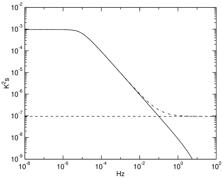
Figure 1: $1/f$ noise power spectrum, as given by expansion (39) and Eq. (41). The solid line shows the pure $1/f$ noise spectrum. The dashed line shows the white noise level ($P_{\rm wn}=\sigma^{2}/f_{\mathrm{s}}$). The dash-dotted line shows the total noise spectrum, including both components. The parameters were $\sigma=2700$ $\mu$K, $f_{\mathrm{s}}=76.8$ Hz, $f_{\mathrm{kn}}=0.1$ Hz, $\Delta=1$, $f_{\mathrm{min}}=10^{-5}$ Hz, $f_{\mathrm{max}}=10$ Hz.

4.3 Component covariance matrices

In this section we give explicit formulae for the elements of the component covariance matrix $\mathbf{C}^{k}$ that corresponds to the auto-correlation function (37). Derivation is given in Appendix A. Here we just quote the results.

We use again the index notation, where indices $i,i^{\prime}$ refer to rings and $l,l^{\prime}$ to base functions. The elements of the component covariance matrix are given by

$$C^{k}_{ii^{\prime}ll^{\prime}}=G_{k}S^{+}_{kl}S^{-}_{kl^{\prime}}\exp\big{(}-\frac{g_{k}}{f_{\mathrm{sp}}}(i-i^{\prime}-1)M\big{)}\quad(i>i^{\prime})$$ (43)

$$C^{k}_{ii^{\prime}ll^{\prime}}=G_{k}S^{-}_{kl}S^{+}_{kl^{\prime}}\exp\big{(}-\frac{g_{k}}{f_{\mathrm{sp}}}(i^{\prime}-i-1)M\big{)}\quad(i<i^{\prime})$$ (44)

$$C^{k}_{ii^{\prime}ll^{\prime}}=\frac{1}{M}\sum_{j=0}^{n-1}\big{(}\bar{F}_{lj}\bar{F}_{l^{\prime}j}+\bar{F}_{lj}A_{l^{\prime}j}+\bar{F}_{l^{\prime}j}A_{lj}\big{)}$$

$$\hskip 28.45274pt\qquad+G_{k}^{0}(S^{+}_{kl}S^{-}_{kl^{\prime}}+S^{-}_{kl}S^{+}_{kl^{\prime}}).\qquad(i=i^{\prime})$$

Here $f_{\mathrm{sp}}=f_{\mathrm{s}}/n$, where $n$ is the number of samples on a ring, represents the spin frequency of the instrument. If no coadding is applied, $n$ can be chosen freely, and $f_{\mathrm{sp}}$ does not need to have any connection to the scanning pattern of the instrument. In that case $f_{\mathrm{sp}}$ represents simply the inverse of the chosen baseline length.

Factors $S^{+}$ and $S^{-}$ are defined as

$$S^{+}_{kl}=\sum_{j=0}^{n-1}\bar{F}_{lj}\exp(-\frac{g_{k}}{f_{\mathrm{s}}}j)$$ (46)

$$S^{-}_{kl}=\sum_{j=0}^{n-1}\bar{F}_{lj}\exp(-\frac{g_{k}}{f_{s}}(n-j)).$$ (47)

Coadding brings in the factors

$$G_{k}=\frac{1}{M^{2}}\frac{[1-\exp(-\frac{g_{k}}{f_{\mathrm{sp}}}M)]^{2}}{[1-\exp(-\frac{g_{k}}{f_{\mathrm{sp}}})]^{2}}$$ (48)

and

$$G_{k}^{0}=\frac{1}{M}\frac{1}{1-\exp(-\frac{g_{k}}{f_{\mathrm{sp}}})}\Big{[}1-\frac{1}{M}\frac{1-\exp(-\frac{g_{k}}{f_{\mathrm{sp}}}M)}{1-\exp(-\frac{g_{k}}{f_{\mathrm{sp}}})}\Big{]}$$ (49)

If no coadding is done ($M=1$), we have $G_{k}=1$ and $G_{k}^{0}=0$.

Factor $A_{lj}$ is defined by

$$A_{lj}=\sum_{j^{\prime}=0}^{j-1}\bar{F}_{lj^{\prime}}\exp(-\frac{g_{k}}{f_{\mathrm{s}}}(j-j^{\prime}))$$ (50)

and can be computed rapidly using the recurrence relation

$$A_{lj}=(A_{l,j-1}+\bar{F}_{l,{j-1}})\exp(-\frac{g_{k}}{f_{\mathrm{s}}}),$$ (51)

with the starting value $A_{l0}=0$.

Formulae (43)-(4.3) are very fast to evaluate numerically, as compared to the general formula (4.1).

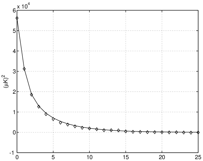
Figure 2: Covariance between uniform baselines, as a function of the distance between rings. The solid line shows the theoretical curve, computed using Eqs. (43)-(4.3). Diamonds present the values determined from simulated noise. The noise parameters were $\sigma=2700$ $\mu$K, $f_{\mathrm{s}}=76.8$ Hz, $f_{\mathrm{kn}}=0.1$ Hz, $\Delta=1$, $f_{\mathrm{min}}=10^{-5}$ Hz, $f_{\mathrm{max}}=10$ Hz.

Table 2: The first elements of the covariance matrix $\mathbf{C}_{a}$ (in ($\mu$K)²). The noise parameters were the same as in Fig. 2. We used Fourier components as base functions, normalized as $\sum_{j}F_{lj}^{2}=n$. We show elements $l,l^{\prime}=1\ldots 5$ and $i-i^{\prime}=0\ldots 3$. Index value $l=1$ refers to the uniform baseline and values $l=2$ and $l=3$ ($l=4$ and $l=5$) to the sine and cosine of the first (second) Fourier mode, respectively. The noise parameters were the same as in Fig. 2.

$l$	i-i’	$l^{\prime}=1$	$l^{\prime}=2$	$l^{\prime}=3$	$l^{\prime}=4$	$l^{\prime}=5$
1	0	56049	0	-2.41	0	-0.668
	1	31324	-89.6	1.10	-44.9	0.307
	2	18707	-28.9	0.0531	-14.5	0.0133
	3	12928	-16.3	0.0210	-8.17	5.25e-3
2	0	0	161	0	1.64	0
	1	89.6	-1.42	0.209	-0.745	0.0696
	2	28.9	-0.0751	2.35e-4	-0.0376	5.88e-5
	3	16.3	-0.0297	5.90e-5	-0.0148	1.48e-5
3	0	-2.41	0	158	0	-0.123
	1	1.10	-0.209	0.133	-0.139	0.0617
	2	0.0531	-2.35e-4	1.14e-6	-1.18e-4	2.85e-7
	3	0.0210	-5.90e-5	1.73e-7	-2.95e-5	4.32e-8
4	0	0	1.64	0	79.9	0
	1	44.9	-0.745	0.139	-0.401	0.0524
	2	14.5	-0.0376	1.18e-4	-0.0188	2.94e-5
	3	8.17	-0.0148	2.95e-5	-7.42e-3	7.38e-6
5	0	-0.668	0	-0.123	0	79.0
	1	0.307	-0.0696	0.0617	-0.0524	0.0334
	2	0.0133	-5.88e-5	2.85e-7	-2.94e-5	7.13e-8
	3	5.25e-3	-1.48e-5	4.32e-8	-7.38e-6	1.08e-8

Figure 2 presents the theoretical covariance, computed using expansion (38), between uniform baselines for $1/f$ noise with $f_{\mathrm{kn}}=0.1$ Hz. Other parameters used were $f_{\mathrm{s}}=76.8$ Hz, $f_{\mathrm{sp}}=1/60$ Hz, $n=4608$ and $M=60$. We show in the same figure the covariance as determined from simulated $1/f$ noise. We generated 10 realizations of noise TOD of one year length, and computed their auto-correlation using the Fourier technique. The agreement is very good.

As another example we show in Table 2 the first elements of the covariance matrix for Fourier components. Index $l=1$ refers to the uniform baseline and indices $l=2$ and $l=3$ ($l=4$ and $l=5$) to the sine and cosine of the first (second) Fourier mode, respectively. We have normalized all components to $\sum_{j}F_{lj}^{2}=n$. Elements of matrix $\mathbf{F}$ are thus $F_{1j}=1$, $F_{2j}=\sqrt{2}\sin(2\pi j/n)$, $F_{3j}=\sqrt{2}\cos(2\pi j/n)$, $F_{4j}=\sqrt{2}\sin(4\pi j/n)$, $F_{5j}=\sqrt{2}\cos(4\pi j/n)$, and $\bar{\mathbf{F}}$ is given by $\bar{F}_{lj}=F_{lj}/n$. We see that the dominant elements are those corresponding to uniform baselines.

5 Simulation results

5.1 Data sets

We have produced two sets of simulated TOD. We refer to them as ’coadded’ and ’uncoadded’ data sets.

The coadded data set mimicks the one year TOD from one Planck LFI 70 GHz detector. The scanning pattern was the following. The spin axis remained in the equatorial plane and was turned 2.4 arcmin every hour, so that after 8640 hours the spin axis had turned 360 degrees. The detector turned around the spin axis with an opening angle of 85 $\deg$ and spin frequency $f_{\mathrm{sp}}=1/60$ Hz. The sampling frequency was $f_{\mathrm{s}}=76.8$ Hz. We coadded data of 60 consecutive spin circles to form a ring. Our total data set consisted of 8640 rings, with 4608 samples in each. The sky coverage was 0.9964.

The uncoadded data set was generated with a quite similar scanning pattern. The main difference was that instead of moving in steps, the spin axis turned continuously at the rate of 360 degrees in 8640 min. The sampling and spin frequencies as well as the opening angle were the same as in the first data set. Because the spin axis moved continuously, consecutive circles did not fall on top of each other, and no coadding was done. The total length of the TOD was the same as in the coadded data set, i.e. 8640$\times$4608 samples. The amount of data was equivalent to 6 days of one detector Planck data, spread over the whole sky. This scanning pattern was rather artificial, but our purpose was only to demonstrate the use of MADAM in the case of uncoadded data. Full-scale simulations with realistic uncoadded one-year Planck data are beyond the scope of this paper.

The underlying CMB map was created by the Synfast code of the HEALPix package (Górski et al. 1999, 2004), starting from the CMB anisotropy angular power spectrum computed with the CMBFAST code (Zeljak & Zaldarriaga 1996) using the cosmological parameters $\Omega_{\rm tot}=1.00$, $\Omega_{\Lambda}=0.7$, $\Omega_{\mathrm{b}}h^{2}=0.02$, $h=0.7$, $n=1.00$, and $\tau=0.0$. We created the input map with HEALPix resolution $N_{\mathrm{side}}=2048$ and with a symmetric Gaussian beam with full width at half maximum (FWHM) of 14 arcmin. We then formed the signal TOD by picking temperatures from this map. Our output maps have resolution parameter $N_{\mathrm{side}}$=512, corresponding to an angular resolution of 7 arcmin.

We used the Stochastic Differential Equation (SDE) technique to create the instrument noise stream, which we added to the signal TOD. We generated noise with power spectrum

$$P(f)=\left(1+\frac{f_{\mathrm{kn}}}{f}\right)\frac{\sigma^{2}}{f_{\mathrm{s}}},\quad(f>f_{\mathrm{min}})$$ (52)

with parameters $\sigma=2700$ $\mu$K, knee frequency $f_{\mathrm{kn}}=0.1$ Hz, and $f_{\mathrm{min}}=10^{-5}$ Hz. The white noise level 2700 $\mu$K (CMB temperature scale) corresponds to the estimated white noise level of one 70 GHz LFI detector. We used the same noise spectrum for both data sets.

We run our code on one processor of an IBM eServer Cluster 1600 supercomputer.

5.2 Results for coadded data

We show our results for the coadded data set in Tables 3-5. As a figure of merit we have used the rms of the residual noise map. The residual noise map was computed by subtracting from the output map a reference map. The reference map was created by coadding the pure signal TOD into a map. We then subtracted the monopole from the residual map and computed its rms value.

Table 3: Average rms of the residual noise map for different numbers of base functions, for coadded data. We fit Fourier components and Legendre polynomials. The averages are taken over 10 noise realizations. We show also the number of iteration steps and CPU time in the Fourier case.

	Legendre	Fourier
$L$	rms$/\mu$K	rms$/\mu$K	iter	CPU/s
1	110.634	110.634	16	59
2	110.560
3	110.525	110.485	20	65
4	110.481
5	110.451	110.422	28	106
7	110.413	110.386	28	123
9	110.387	110.363	32	164
11	110.368	110.347	32	191
15	110.344	110.326	36	267
25	110.312	110.301	40	530
35	110.298	110.290	44	758
45	110.290	110.283	52	1154
65		110.277	56	1959

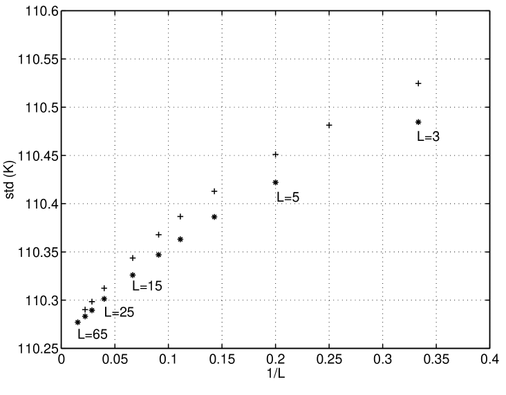
Figure 3: Rms of the residual noise map plotted against the inverse of the number of base functions, for Legendre polynomials (+) and Fourier components (*). The numerical values are given in Table 3. The std seems to converge towards value 110.26 $\mu$K at the limit $L\rightarrow n$.

The results for different numbers of base functions are given in Table 3. The given rms values are averages over 10 noise realizations. We tried two sets of base functions: Fourier components and Legendre polynomials. Because a Fourier fit always includes an uniform baseline plus an equal number of sine and cosine functions, the total number $L$ of base functions is always an odd number. The rms values continue improving when we increase the number of base functions. Fourier components give lower rms values than Legendre polynomials for the same number of components. In the rest of the simulations in this section we fitted only Fourier components.

We show also the number of iterations and total CPU time taken by one run in the case of Fourier components. Since the CPU time naturally depends on the computer used and may vary from run to run, the values quoted should not be taken too seriously. They merely give an idea how the run time increases with increasing number of base functions.

In Fig. 3 we have plotted the rms values against the inverse of the number of base functions. At the limit $1/L\rightarrow 0$ the rms values seem to be approaching the value 110.26 $\mu$K. We expect that to be the std of the minimum-variance map (Section 2.2). The expected contribution from white noise to the residual map rms is 108.95 $\mu$K. This value was computed from the white noise sigma and the known distribution of measurements in the sky.

We have compared results of fitting uniform baselines using MADAM and ordinary destriping technique. We got the destriping results by running MADAM with $\mathbf{C}_{a}^{-1}=0$. At this limit the method reduces to pure destriping. The destriping result was 110.63444 $\mu$K (110.63443 $\mu$K with MADAM). This indicates that when fitting uniform baselines only, the covariance plays very little role, but the baselines can be determined from the data alone with good accuracy.

Keihänen et al. (2004) showed that fitting Fourier components beyond the uniform baseline with the ordinary destriping technique, without using the covariance matrix, did not improve the results. In this work we have found a clear improvement. This indicates, that information about the noise spectrum is important when fitting base functions other than the uniform baseline.

Table 4: Effect of misestimating the noise spectrum. We show the average residual map std (in $\mu$K) for different numbers of Fourier components and for different assumed knee frequencies $f_{\mathrm{kn}}$ (upper panel), spectral slopes $\gamma$ (middle), and minimum frequencies $f_{\mathrm{min}}$ (lower panel). The other two noise parameters were kept at their correct values ($f_{\mathrm{kn}}=0.1$ Hz, $\gamma=-1.0$, and $f_{\mathrm{min}}=10^{-5}$ Hz). The lowest rms value on each row is denoted by an asterisk. The correct parameter value is shown in boldface.

		$f_{\mathrm{kn}}$
L	0.03 Hz	0.05 Hz	0.1 Hz	0.2 Hz
1	110.634*	110.634*	110.634*	110.634*
3	110.492	110.484*	110.485	110.492
5	110.436	110.420*	110.422	110.441
7	110.409	110.387	110.386*	110.411
9	110.392	110.366	110.363*	110.393
11	110.382	110.353	110.347*	110.380
15	110.369	110.335	110.326*	110.363
25	110.355	110.319	110.301*	110.344
		$\gamma$
L	-0.6	-0.8	-1.0	-1.2
1	110.640	110.635	110.634*	110.634
3	110.490	110.483*	110.485	110.488
5	110.428	110.419*	110.422	110.428
7	110.394	110.384*	110.386	110.393
9	110.373	110.361*	110.363	110.369
11	110.359	110.346*	110.347	110.352
15	110.340	110.326*	110.326*	110.330
25	110.321	110.303	110.301*	110.304
35	110.314	110.293	110.290*	110.292
		$f_{\mathrm{min}}$
L	$10^{-6}$ Hz	$\mathbf{10^{-5}}$ Hz	$10^{-4}$ Hz	$10^{-3}$ Hz
1	110.634*	110.634*	110.635	110.655
3	110.485*	110.485*	110.485	110.510
5	110.422*	110.422*	110.422	110.463
7	110.386*	110.386*	110.386	110.433
9	110.363*	110.363*	110.363	110.415
11	110.347*	110.347*	110.347	110.402
15	110.326*	110.326*	110.326	110.386
25	110.301*	110.301*	110.302	110.367

We have also studied the effect of misestimating the noise spectrum. We varied in turn each of the three noise parameters (knee frequency, spectral slope, and minimum frequency) while keeping the other two at their correct values ($f_{\mathrm{kn}}=0.1$ Hz, $\gamma=-1.0$, $f_{\mathrm{min}}=10^{-5}$ Hz). We then recomputed the covariance matrix $\mathbf{C}_{a}$ with the new parameter values and rerun the map estimation. We fitted Fourier components only. The results are shown in Table 4.

It is perhaps surprising that for small $L$ underestimating the knee frequency or assuming a less deep slope seems to improve the results. This can be understood as follows. When $L$ is small, the noise is not perfectly modelled by the base functions. There is an error involved, related to the higher Fourier components that have not been included in the analysis. This error affects the estimation of the lower components, leading to a too high variation in their amplitudes. The error in the covariance matrix, caused by misestimation of the noise spectrum, partly compensates for this error. We notice that the best results are obtained with a spectrum (less deep a slope or lower knee frequency) which leads to a smaller covariance for the low-frequency Fourier components. Smaller covariance tends to restrict the variation of the amplitudes, thus decreasing their error also. With larger $L$ the phenomenon disappears, and the lowest rms is obtained with the correct noise spectrum, as expected.

Table 5: Pixelization noise. Rms of the residual map for noise-free TOD. The error is due to finite pixelization of the sky.

$L$	rms/$\mu$K
1	0.138
3	0.207
5	0.233
7	0.257
9	0.274
11	0.289
15	0.319
25	0.359
35	0.380
45	0.393

Table 5 shows results from a run with noise-free data. The TOD contained only the contribution from the CMB signal, but no instrument noise. The error that still remains in the map is due to ’pixelization noise’ (Doré et al. 2001) caused by the finite size of sky pixels. The pixelization error increases with increasing number of base functions, but is very small compared with the error due to instrument noise.

5.3 Results for uncoadded data

If no coadding is applied, the length $n$ of a ring is not determined by the scanning pattern of the instrument, but is a free parameter to be chosen at will. We then have two parameters to select: the number $L$ of base functions and their length $n$.

To keep things simple, we tried two schemes. First we kept the baseline length fixed at one minute and varied the number of Fourier components that we fitted. Secondly, we fitted uniform baselines only ($L=1$) but varied their length.

Results from the first case are shown in Table 6. The baseline length was fixed at $n=4608$ samples (one minute). We show again the average rms of the residual noise map, averaged over 10 realizations of noise. The white noise level is higher than in the coadded case by a factor of $\sqrt{60}$. The expected white noise contribution to the map rms is 844.0 $\mu$K.

Table 7 shows results of fitting uniform baselines of different lengths. The first column gives the length $n$ of the baseline, as the number of samples. The second column gives the baseline length in seconds. The third column shows the number of baselines per minute ($4608/n$). The shortest baseline we tried consisted of only 9 samples.

The third column of Table 7 and the first column of Table 6 are comparable, since they give the total number of unknows per one minute of TOD. We see that for a given number of unknowns, fitting Fourier components works better than fitting uniform baselines. However, when we compare CPU times, we see that fitting uniform baselines is more effective.

Table 6: Average residual noise rms for different numbers of Fourier components, for the uncoadded data set. The ring length was $n=4608$. Also shown are the number of iteration steps and the CPU time for one run.

$L$	rms/$\mu$K	iter	CPU/s
1	857.131	28	68
3	855.782	36	102
5	855.294	48	161
7	838.373	52	205
9	854.842	56	280
11	854.718	60	336
15	854.555	64	436
25	854.357	76	847

Table 7: Results of fitting uniform baselines of different lengths to uncoadded data. The first three columns give the baseline length as the number of samples and in seconds, respectively, and the number of baselines per one minute of TOD. The next columns give the average residual noise rms, number of iteration steps and total CPU time taken by one run.

$n$	$t$/s	N/min	rms/$\mu$K	iter	CPU/s
4608	60.0	1	857.131	28	68
2304	30.0	2	856.220	32	80
1152	15.0	4	855.837	36	96
576	7.5	8	855.202	48	123
288	3.75	16	854.769	64	150
144	1.88	32	854.463	84	215
72	0.94	64	854.271	116	331
36	0.47	128	854.169	160	672
18	0.23	256	854.116	224	1284
9	0.12	512	854.092	320	2889

Table 8: Comparison between MADAM and destriping.

			MADAM	destriping
$n$	$t$/s	N/min	rms/$\mu$K	rms/$\mu$K
4608	60.0	1	857.131	857.135
2304	30.0	2	856.220	856.239
1152	15.0	4	855.837	856.779
576	7.5	8	855.202	861.118
288	3.75	16	854.769	875.798

As in the case of coadded data, we compared results of fitting uniform baselines using MADAM and ordinary destriping technique. The results are shown in Table 8. With one minute baselines the difference between the methods is small, but increases with decreasing $n$, in favour of MADAM. The rms value obtained with destriping reaches a minimum around 0.5 min baseline length, while with MADAM the values continue improving. With small values of $n$ MADAM is clearly superior to basic destriping.

6 Conclusions

We have presented a new map-making method for CMB experiments called MADAM. The method is based on the well known destriping technique, but unlike basic destriping, it also uses information on the known statistical properties of the instrument noise in the form of the covariance matrix of the base function amplitudes. We have shown that with this extra information the CMB map can be estimated with better accuracy than with pure destriping.

We have tested the method with simulated coadded Planck -like data. As a figure of merit we have used the rms of the residual noise map. Our simulations show that fitting more base functions clearly improves the accuracy of the output map, with the cost of increasing requirements for CPU time and memory.

We have shown theoretically that the map estimate given by MADAM approaches the optimal minimum-variance map when the number of fitted base functions increases. In practice it is not possible to reach the exact minimum-variance map using MADAM, due to CPU time and memory limitations. Still, MADAM provides a fast and efficient map-making method. By varying the number of base functions the user may flexibly move from a very fast but less accurate map-making (small $L$) to a more accurate but more time-consuming map-making (large $L$), depending on what is desired.

We also demonstrated the use of MADAM for uncoadded data. Although the data set used was quite artificial, in the sense that it does not mimick data from any existing CMB experiment, the method was shown to work well for uncoadded data also.

The current implementation of the method is a serial one. With a parallelized version we expect to be able to process data sets equivalent to full-year uncoadded Planck data.

Appendix A Covariance matrix for a power-law power spectrum

We discussed the computation of the covariance matrix $\mathbf{C}_{a}$ in Section 4. In this appendix we present some technical calculations which were omitted there.

A.1 Exponential expansion for a power-law spectrum

Assume that the auto-correlation function of the noise can be expanded as

$$c(t)=\sum_{k}b_{k}\exp(-g_{k}|t|)$$ (53)

where and $g_{k}$ is a selected set of characteristic frequencies. We now derive the coefficients $b_{k}$ in the case of a power-law power spectrum of the form

$$P(f)\propto f^{\gamma}$$ (54)

for $-2\leq\gamma<0$.

The power spectrum $P(f)$ and the auto-correlation function $c(t)$ of stationary noise are related by the cosine transform

$$P(f)=\int_{-\infty}^{\infty}c(t)\cos(2\pi ft)dt.$$ (55)

The auto-correlation function $\exp(-g|t|)$ corresponds to the power spectrum

$$P(f,g)=\frac{2g}{g^{2}+(2\pi f)^{2}}.$$ (56)

The total power spectrum corresponding to the auto-correlation (53) is given by

$$P(f)=\sum_{k}b_{k}P(f,g_{k})=\sum_{k}\frac{2b_{k}g_{k}}{g_{k}^{2}+(2\pi f)^{2}}.$$ (57)

We pick the frequencies $g_{k}$ uniformly in logarithmic scale inside some range $[f_{\mathrm{min}},f_{\mathrm{max}}]$ and use the ansatz

$$b_{k}=Ag_{k}^{\gamma+1}\Delta$$ (58)

where $\Delta=\ln(g_{k+1}/g_{k})$ is the logarithmic step in $g$ and $A$ is a constant to be determined. The total power spectrum becomes

$$P(f)=A\sum_{k}\frac{2g_{k}^{\gamma+2}}{g_{k}^{2}+(2\pi f)^{2}}\Delta.$$ (59)

We transform the sum into an integral

$$P(f) = A\int_{f_{\mathrm{min}}}^{f_{\mathrm{max}}}\frac{2g^{\gamma+2}}{g^{2}+(2\pi f)^{2}}\frac{dg}{g}$$

$$\approx A\int_{0}^{\infty}\frac{2g^{\gamma+1}}{g^{2}+(2\pi f)^{2}}dg\quad(f_{\mathrm{min}}\ll f\ll f_{\mathrm{max}}).$$

The integral converges for $-2<\gamma<0$,

$$P(f)=A\frac{\pi(2\pi f)^{\gamma}}{\sin[(\gamma+2)\pi/2]}\quad\propto\,f^{\gamma}.$$ (61)

We choose

$$A=\frac{\sigma^{2}}{f_{\mathrm{s}}}\frac{1}{\pi}(2\pi f_{\mathrm{kn}})^{-\gamma}\sin[(\gamma+2)\pi/2]$$ (62)

to obtain the desired power spectrum

$$P(f)=\frac{\sigma^{2}}{f_{\mathrm{s}}}(\frac{f}{f_{\mathrm{kn}}})^{\gamma}\qquad(f_{\mathrm{min}}\ll f\ll f_{\mathrm{max}}).$$ (63)

Here $\sigma$ is the white noise std, $f_{\mathrm{s}}$ is the sampling frequency, and $f_{\mathrm{kn}}$ is the knee frequency, at which the power of the power-law noise component equals the white noise power $\sigma^{2}/f_{\mathrm{s}}$. The maximum $f_{\mathrm{max}}$ should well exceed the knee frequency.

The coefficients $b_{k}$ are given by

$$b_{k}=\frac{\sigma^{2}}{f_{\mathrm{s}}}\frac{1}{\pi}(2\pi f_{\mathrm{kn}})^{-\gamma}\sin[(\gamma+2)\pi/2]g_{k}^{\gamma+1}\Delta$$ (64)

for $-2<\gamma<0$. Especially, for $1/f$ noise ($\gamma=-1$) we have the simple formula

$$b_{k}=2\sigma^{2}\frac{f_{\mathrm{kn}}}{f_{\mathrm{s}}}\Delta.$$ (65)

The case $\gamma=-2$ requires a separate treatment. We see directly from Eq. (56), that the desired spectrum is given by one single $g$ component with coefficient

$$b=\frac{2\pi^{2}f_{\mathrm{kn}}^{2}}{g}\frac{\sigma^{2}}{f_{\mathrm{s}}}.$$ (66)

The spectrum then has the form

$$P(f)=\frac{f_{\mathrm{kn}}^{2}}{f_{\mathrm{min}}^{2}+f^{2}}\frac{\sigma^{2}}{f_{\rm s}}$$ (67)

where $f_{\mathrm{min}}=g/(2\pi)$. The spectrum behaves as $\propto f^{-2}$ at $f\gg f_{\mathrm{min}}$ and levels out below $f_{\mathrm{min}}$.

A.2 Component covariance matrices

Once the expansion (53) has been found, the covariance matrix can be computed as

$$\mathbf{C}_{a}=\sum_{k}b_{k}\mathbf{C}^{k}.$$ (68)

In the following we calculate the component covariance matrices $\mathbf{C}^{k}$.

In Section 4 we derived the general formula

$$C_{ii^{\prime}ll^{\prime}}=$$

$$\sum_{j,j^{\prime}=0}^{n-1}\bar{F}_{lj}\bar{F}_{l^{\prime}j^{\prime}}\frac{1}{M^{2}}\sum_{m,m^{\prime}=0}^{M-1}c_{[(i-i^{\prime})nM+(m-m^{\prime})n+j-j^{\prime}]}.$$

Assume then that the auto-correlation function is of the exponential form

$$\langle y_{p}y_{p^{\prime}}\rangle=c_{k,p-p^{\prime}}=\exp(-g_{k}|t|)=\exp\big{(}-\frac{g_{k}}{f_{\mathrm{s}}}|p-p^{\prime}|\big{)}$$ (70)

where $f_{\mathrm{s}}$ is the sampling frequency and indices $p,p^{\prime}$ label samples along the TOD. We substitute this into Eq. (A.2). The covariance becomes

$$C^{k}_{ii^{\prime}ll^{\prime}} = \sum_{jj^{\prime}=0}^{n-1}\bar{F}_{lj}\bar{F}_{l^{\prime}j^{\prime}}\frac{1}{M^{2}}\sum_{m,m^{\prime}=0}^{M-1}$$

$$\times\exp\big{(}-\frac{g_{k}}{f_{\mathrm{s}}}|(i-i^{\prime})nM+(m-m^{\prime})n+j-j^{\prime}|\big{)}.$$

We treat cases $|i-i^{\prime}|>0$ and $i=i^{\prime}$ separately.

1. $|i-i^{\prime}|>0$. If $i-i^{\prime}>0$ the quantity inside the brackets is positive, and we can split the four-dimensional sum into a product of four sums as

   $$C^{k}_{ii^{\prime}ll^{\prime}} = \exp\big{(}-\frac{g_{k}}{f_{\mathrm{s}}}(i-i^{\prime}-1)nM\big{)}$$ (72)

   $$\times\frac{1}{M^{2}}\sum_{m=0}^{M-1}{\rm e}^{-\frac{g_{k}}{f_{\mathrm{s}}}mn}\sum_{m=0}^{M-1}{\rm e}^{-\frac{g_{k}}{f_{\mathrm{s}}}(M-1-m)n}$$

   $$\times\sum_{j=0}^{n-1}\bar{F}_{lj}{\rm e}^{-\frac{g_{k}}{f_{\mathrm{s}}}j}\sum_{j^{\prime}=0}^{n-1}\bar{F}_{l^{\prime}j^{\prime}}{\rm e}^{-\frac{g_{k}}{f_{\mathrm{s}}}(n-j^{\prime})}.$$

   We have arranged the terms in such a way that the argument of an exponent function is always negative. This is helpful in numerical evaluation. The sum over $m,m^{\prime}$ can be carried out analytically, yielding

   $$G_{k} = \frac{1}{M^{2}}\sum_{m=0}^{M-1}{\rm e}^{-\frac{g_{k}}{f_{\mathrm{s}}}mn}\sum_{m=0}^{M-1}{\rm e}^{-\frac{g_{k}}{f_{\mathrm{s}}}(M-1-m)n}$$ (73)

   $$= \frac{1}{M^{2}}\frac{(1-{\rm e}^{-\frac{g_{k}}{f_{\mathrm{sp}}}M})^{2}}{(1-{\rm e}^{-\frac{g_{k}}{f_{\mathrm{sp}}}})^{2}}$$

   where $f_{\mathrm{sp}}=f_{\mathrm{s}}/n$.

   The elements for which $i-i^{\prime}<0$ are obtained from the symmetry relation,$C^{k}_{ii^{\prime}ll^{\prime}}=C^{k}_{i^{\prime}il^{\prime}l}$.

2. The case $i=i^{\prime}$ is more complicated, since the quantity inside the brackets in Eq. (A.2) takes both positive and negative values. We split the sum into three terms ($m=m^{\prime}$, $m>m^{\prime}$, and $m<m^{\prime}$) and the $m=m^{\prime}$ term further into three terms ($j=j^{\prime}$, $j>j^{\prime}$, and $j<j^{\prime}$),

   $$C^{k}_{iill^{\prime}} = \sum_{jj^{\prime}=0}^{n-1}\bar{F}_{lj}\bar{F}_{l^{\prime}j^{\prime}}\frac{1}{M^{2}}\sum_{m,m^{\prime}=0}^{M-1}\ {\rm e}^{-\frac{g_{k}}{f_{\mathrm{s}}}|(m-m^{\prime})n+j-j^{\prime}|}$$ (74)

   $$= \frac{1}{M^{2}}\sum_{m=0}^{M-1}\sum_{m^{\prime}<m}{\rm e}^{-\frac{g_{k}}{f_{\mathrm{s}}}(m-m^{\prime}-1)n}$$

   $$\quad\times\sum_{j=0}^{n-1}\bar{F}_{lj}{\rm e}^{-\frac{g_{k}}{f_{\mathrm{s}}}j}\sum_{j^{\prime}=0}^{n-1}\bar{F}_{l^{\prime}j^{\prime}}{\rm e}^{-\frac{g_{k}}{f_{\mathrm{s}}}(n-j^{\prime})}$$

   $$+ \frac{1}{M^{2}}\sum_{m^{\prime}=0}^{M-1}\sum_{m<m^{\prime}}{\rm e}^{-\frac{g_{k}}{f_{\mathrm{s}}}(m^{\prime}-m-1)n}$$

   $$\quad\times\sum_{j=0}^{n-1}\bar{F}_{lj}{\rm e}^{-\frac{g_{k}}{f_{\mathrm{s}}}(n-j)}\sum_{j^{\prime}=0}^{n-1}\bar{F}_{l^{\prime}j^{\prime}}{\rm e}^{-\frac{g_{k}}{f_{\mathrm{s}}}j}$$

   $$+ \frac{1}{M}\sum_{j=0}^{n-1}\bar{F}_{lj}\bar{F}_{l^{\prime}j}+\frac{1}{M}\sum_{j=0}^{n-1}\bar{F}_{lj}\sum_{j^{\prime}<j}\bar{F}_{l^{\prime}j^{\prime}}{\rm e}^{-\frac{g_{k}}{f_{\mathrm{s}}}(j-j^{\prime})}$$

   $$+ \frac{1}{M}\sum_{j^{\prime}=0}^{n-1}\bar{F}_{l^{\prime}j^{\prime}}\sum_{j<j^{\prime}}\bar{F}_{lj}{\rm e}^{-\frac{g_{k}}{f_{\mathrm{s}}}(j^{\prime}-j)}.$$

   The sum over $m,m^{\prime}$ can again be calculated analytically,

   $$G_{k}^{0} = \frac{1}{M^{2}}\sum_{m=0}^{M-1}\sum_{m^{\prime}<m}\exp(-\frac{g_{k}}{f_{\mathrm{sp}}}(m-m^{\prime}-1))$$

   $$= \frac{1}{M}\frac{1}{1-\exp(-\frac{g_{k}}{f_{\mathrm{sp}}})}\Big{[}1-\frac{1}{M}\frac{1-\exp(-\frac{g_{k}}{f_{\mathrm{sp}}}M)}{1-\exp(-\frac{g_{k}}{f_{\mathrm{sp}}})}\Big{]}.$$

   Formula (74) may seem complicated, but is easy and fast to evaluate numerically.

Equations (72) and (74), when written in compact form, give the formulae (43)-(4.3) in Section 4.

References

- Burigana (1997) Burigana C., Malaspina M., Mandolesi N., Danese L., Maino D., Bersanelli M., Maltoni M., 1997, Int. Rep. TeSRE/CNR, 198/1997, November, (astro-ph/9906360)
- Delabrouille (1998) Delabrouille J., 1998, A&AS, 127, 555
- Maino (1999) Maino D. et al., 1999, A&AS, 140, 383
- Maino (2002) Maino D., Burigana C., Górski K.M., Mandolesi N., Bersanelli M., 2002, A&A, 387, 356
- Keihänen (2004) Keihänen E., Kurki-Suonio H., Poutanen T., Maino D., Burigana C., 2004, A&A, 428, 287
- Natoli (2001) Natoli P., de Gasperis G., Gheller C., Vittorio N., 2001, A&A, 372, 346
- Doré (2001) Doré O., Teyssier R., Bouchet F.R., Vibert D., Prunet S. 2001, A&A, 374, 358
- Borrill (1999) Borrill, J. 1999, preprint (astro-ph/9911389)
- Górski (1999) Górski K.M., Hivon E., Wandelt B.D., 1999, in Proceedings of the MPA/ESO Cosmology Conference ”Evolution of Large-Scale Structure”, ed. A.J. Banday, R.S. Sheth, & L. Da Costa, PrintPartners Ipskamp, NL, 37, (astro-ph/9812350)
- Górski (2004) Górski K.M., Hivon E., Banday A.J., Wandelt B.D., Hansen F.K., Reinecke M., Bartelman M., 2004, preprint (astro-ph/0409513)
- Press (1992) Press W.H., Teukolsky S.A., Vetterling W.T., Flannery B.P., 1992, Numerical Recipes, 2nd ed. (Cambridge University Press, Cambridge)
- Seljak (1996) Seljak U., Zaldarriaga M., 1996, ApJ, 469, 437