Study the X-ray Dust Scattering Halos with Chandra Observations of Cygnus X-3 and Cygnus X-1

Abstract

We improve the method proposed by Yao et al (2003) to resolve the X-ray dust scattering halos of point sources. Using this method we re-analyze the Cygnus X-1 data observed with Chandra (ObsID 1511) and derive the halo radial profile in different energy bands and the fractional halo intensity (FHI) as $I(E)=0.402\times E_{{\rm keV}}^{-2}$. We also apply the method to the Cygnus X-3 data (Chandra ObsID 425) and derive the halo radial profile from the first order data with the Chandra ACIS+HETG. It is found that the halo radial profile could be fit by the halo model MRN (Mathis, Rumpl $\&$ Nordsieck, 1977) and WD01 (Weingartner $\&$ Draine, 2001); the dust clouds should be located at between 1/2 to 1 of the distance to Cygnus X-1 and between 1/6 to 3/4 (from MRN model) or 1/6 to 2/3 (from WD01 model) of the distance to Cygnus X-3, respectively.

1 Introduction

X-ray halos are formed by the small-angle scatterings of X-rays off dust grains in the interstellar medium. The scatterings are significantly affected by (a) the energy of radiation; (b) the optical depth of the scattering, due to the effects of multiple scatterings; (c) the grain size distribution and compositions; and (d) the spatial distribution of dusts along the line of sight (Mathis $\&$ Lee, 1991, Mathis, Rumpl $\&$ Nordsieck, 1977). Analyzing the properties of X-ray halos is an important tool to study the interstellar grains, which plays a central role in the astrophysical study of the interstellar medium, such as the thermodynamics and chemistry of the gas and the dynamics of star formation.

Before Chandra was lunched, it has been very difficult to get the accurate physical parameters of the X-rays halos due to the poor angular resolution of the previous instruments. With excellent angular resolution, good energy resolution and broad energy band, the Chandra ACIS is so far the best instrument for studying the X-ray halos. However, the direct images of bright sources obtained with ACIS usually suffer from severe pile-up. Although the data in CC-mode or HETGs have either no or less serious pileup, the data in CC mode have only one dimensional images and the data in HETGs are mixed with different energies and radius data, from which we can not get the halo’s radial profile directly. By making use of the assumption that the real halo should be an isotropic image, we have reported the reconstruction of the images of X-ray halos from the data obtained with the HETGS and/or in CC mode. The detailed method has been described in Yao et al. (2003, here after Paper I).

In this paper, we improve the method to resolve the X-ray dust scattering halos of point sources which is proposed in Paper I. The method can resolve the halo more accurately than the method in Paper I, even when some data are contaminated. Furthermore, we modify the method to create the PSF of Chandra. These will be shown in section 2. Using this method we reanalyze the Cygnus X-1 data and also apply the new method to the Cygnus X-3 data, which will be shown in section 3. Finally we give our conclusions and make some discussions in section 4.

2 The method, point spread function and simulation

In Paper I, we have reported that if the flux of a point source plus its X-ray halo is isotropically distributed and centered at the point source as $F(r)$, and the projection process in which the two-dimensions halo image is projected to one dimension image can be represented by a matrix operator $M(r,d)$, then the projected flux distribution $P(d)$ is

$$P(d)=M(r,d)\times F(r),$$ (1)

where $r$ is the distance from the centroid source position and $d$ is the distance from the projection center (refer ro Fig. 1). After calculating the inverse matrix of the operator $M(r,d)$, we can get the source flux $F(r)$. In CC-mode, we can only get the count rate $C(d)$, but not the flux projection $P(d)$ directly. With the exposure map of CCDs calculated, we can get another equation

$${\rm{exposure}\ \rm{map}\choose\rm{matrix}}\times M(r,d)\times F(r)=M^{\prime}(r,d)\times F(r)=C(d),$$ (2)

where $M^{\prime}(r,d)={\rm{exposure}\ \rm{map}\choose\rm{matrix}}\times M(r,d)$ is another matrix. Because the inverse matrix of the operator $M^{\prime}(r,d)$ may not exist, we use the iterative method to solve the above equations. Using the iterative method, we can get the result even though some data in $P(d)$ or $C(d)$ are imperfect or defected. For example, the large angle data $C(d^{*})$ in CC-mode zeroth order are usually contaminated by the data from the HETGs 1st order. In this case we can set these data $C(d^{*})$ and the corresponding matrix elements of $M(r,d^{*})$ to zero. In the process of reconstruction, we can set some limits based on physical constraints, for example the flux of halo should be larger than zero and the flux in the small angle should be larger than the one in the large angle.

Figure 1: The projection of the photons in zeroth order image along the read-out direction and the projection of the photons along the grating arm.

We use the steepest descent method (Marcos Raydan, et al, 2001) to solve equation 3. Then the iterative process can be expressed as

$$F^{(k+1)}(r)=F^{(k)}(r) + \frac{[C(d)-M^{\prime}(r,d)F^{(k)}(r)]^{T}[C(d)-M^{\prime}(r,d)F^{(k)}(r)]}{[M^{\prime}(r,d)[C(d)-M^{\prime}(r,d)F^{(k)}(r)]]^{T}[C(d)-M^{\prime}(r,d)F^{(k)}(r)]}$$ (3)

$$\times [C(d)-M^{\prime}(r,d)F^{(k)}(r)]$$

and where $F^{(k+1)}(r)$ and $F^{(k)}(r)$ are the values of F(r) in the ($k+1$)th and $k$th iterative loops, $[C(d)-M^{\prime}(r,d)F^{(k)}(r)]^{T}$ is the transpose of the matrix $C(d)-M^{\prime}(r,d)F^{(k)}(r)$. In our iterative process, the loop is stopped when $\frac{1}{N}\sum_{d=1}^{N}(\frac{M^{\prime}(r,d)F(r)-C(d)}{\Delta C(d)})^{2}<0.05$, where $N$ is number of $C(d)$ and $\Delta C(d)$ is the error of $C(d)$.

The accurate Chandra PSF (Point Spread Function) is important for reconstructing the halo accurately. We used the MARX simulator to calculate the PSF, but found that at large angles (above 50 arcsec), the PSF from the MARX simulation is very different from the radial flux profile of a point source without halo. Due to the pile-up for bright point sources in the center, we cannot get the PSF from the observation of a bright point source at small angles (below 3–5 arcsec). Therefore we calculated the PSF from the observation data of bright point sources without halo (for example Her X-1) at large angles and from the MARX simulation at small angles.

To test our method, we produced with MARX 4.0 simulator a point source plus one disk source to mimic a point source with its X-ray halo observed with Chandra ACIS+HETGs in TE mode. The reconstructed halo radial surface brightness distribution is consistent with the simulation input, and the recovered FHI (Fractional Halo Intensity) (49.25%) is also consistent with the input value (50%). We thus conclude that the improved method can resolve the radial profile of the halo accurately.

3 Application to Cygnus X-3 and Cygnus X-1

Cygnus X-3 is an X-ray binary with more than 40$\%$ halo flux in 0.1–2.4 keV (ROSAT energy range) (Predelh et al, 1995). The bright X-ray halo has been used to determine the distance of the source (Predelh, et al, 2000). Cygnus X-3 is so bright that there was severe piled-up in the zeroth order image of Chandra ACIS. We use our method to resolve the halo from the data with the highest statistical quality, which was observed on 2000 April 4 (ObsID 425) with Chandra ACIS+HETGs in TE mode.

We use the first order data (HEG $\pm 1$ and MEG $\pm 1$) within 60 arcsec around the source position. First, we filter the data in selected regions using the CCD energy measurement along the grating arm and generate the exposure map for each energy band and region. Dividing the count images by the exposure map, an image in flux units is produced. Then we project the image along the grating arm and get the projected flux in units of photons cm^-2 s^-1 arcsec^-2 per energy band. Finally, we sum the data from the four regions (HEG $\pm 1$ and MEG $\pm 1$) and derive the projected total flux. With the same procedure, we get the projections of PSFs from other sources with negligible halos observed with Chandra ACIS+HETG in TE mode. In order to improve the statistical quality, we use data from four observations, namely, Her X-1 (ObsID 2749) and PKS 2155-304 (ObsID 337, 3167 and 3706). After extracting the projections of PSF, we obtain the pure halo projections. Finally we calculate the operator matrix and derive the halo radial profile in units of photons cm^-2 s^-1 arcsec^-2. The reconstructed halo radial profile is shown in Fig. 2.

Figure 2: The reconstructed halo radial profile of Cygnus X-3. The squares data are the 1st order projection. The dotted line is the projection of PSF in 1st order, the solid line is the pure halo projection, and the dashed line is the reconstructed halo radial profile multiplied by 10 for clarity. Due to the poor statistical quality, the halo within 4 arcsec is not reconstructed.

Figure 3: The reconstructed halo radial profile of Cygnus X-1. The squares data are the projected flux disribution (counts/s). The solid line is reconstructed flux distribution (convolved by the PSF), the dotted line is the PSF from the MARX 4.0 simulation and the Chandra Her X-1 data (ObsID 2749), and the dashed line is the pure halo radial profile multiplied by 10 for clarity.

Figure 4: The X-ray halo profile of Cygnus X-1, fitted using the halo models MRN and WD01. The solid lines are the models MRN (thick line) and WD01 (thin line) where the dust clouds are located between 1/2 to 1 of the distance to the source. The dashed lines are the models MRN (thick line) and WD01 (thin line) with smoothly distributed dust.

Cygnus X-1, discovered in 1965, is one of the brightest X-ray sources in the sky. There is about 11% halo flux in 0.1-2.4 keV (Predehl & Schmit, 1995). In Paper I, we tested our method on Chandra data of Cygnus X-1. Here we re-analyze the data observed on 2000 January 12 (ObsID 1511) with Chandra ACIS+HETGs in CC-mode with an effective exposure of 12.7 ks.
The zeroth order data are the projection C(d) in units of counts arcsec^-2. Then we calculate the exposure map ${\rm{exposure}\ \rm{map}\choose\rm{matrix}}$ in units of counts cm² s photon^-1 of the CCDs within $2^{{}^{\prime}}$ from the source position. Multiplying the exposure map matrix to the projected matrix $M(r,d)$, we obtain the new matrix $M^{\prime}(r,d)$. Using the iterative method, we derive the radial flux $F(r)$ in units of photons cm^-2 s^-1 arcsec^-2.

For energies above 4.0 keV, the grating arms extend into the $2^{\prime}$ region and the zeroth order data in some bins are contaminated by the grating events. Therefore we set these contaminated bins and the corresponding operator matrix elements to zero. For example, the data between 102 arcsec and 117 arcsec (corresponding to 30-32 bins) in energy region 4.5–5.0 keV and the corresponding matrix elements $M[30:32][*]$ are set to zero. The reconstructed flux distribution, the Chandra PSF and the extracted halo in energy band 1.0–1.5 keV are shown in Fig. 3.

Then, we used the halo models MRN and WD01 to fit our halo radial profile of Cygnus X-1 and Cygnus X-3. The two models have different dust grain size distributions: $n(a)~{}a^{-3.5}$ for MRN and $n(a)$ for WD01 is much more complex (refer to Weingartner $\&$ Draine, 2001). For both sources we find the smoothly distributed dust models cannot describe their halo profiles. Then we change the position of the dust cloud manually in the models to fit the halo profile. The best-fit results suggest that the dust clouds should be located at between 1/2 to 1 of the distance to Cygnus X-1 and between 1/6 to 3/4 (fitted by MRN) or 1/6 to 2/3 (fitted by WD01) of the distance to Cygnus X-3, as shown in Fig. 4 and Fig. 5, respectively.

Figure 5: X-ray halo profiles of Cygnus X-3 at 2.0–2.5 keV and 3.0–3.5 keV fitted using the halo models MRN and WD01. The thick solid line is the MRN model where the dust clouds are located between 1/6 to 3/4 of the distance to the source. The thin solid line is the WD01 model where the dust clouds are located between 1/6 to 2/3 of the distance to the source. The dotted lines are the model MRN (thick line) and WD01 (thin line) with smoothly distributed dust.

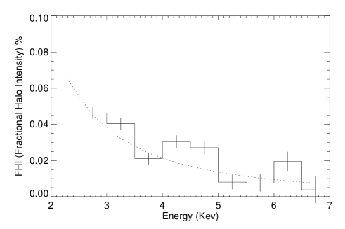
Figure 6: The FHI (relative to the source flux), as a function of energy with the best fit curve $I(E)=(0.339\pm 0.010)\times E_{{\rm keV}}^{-2}$

Finally, we calculate the FHI (Fractional Halo Intensity) of Cygnus X-1 as a function of energy. Using the halo in 120 arcsec instead of the whole halo to derive the FHI, we find

$$I(E)=(0.339\pm 0.010)\times E_{\rm{keV}}^{-2}$$ (4)

as shown in Fig. 6. This is very different from the result derived in Paper I. The main reason is that in Paper I we only used the MARX 3.0 to calculate the PSF whose contribution is under-estimated at large angles, especially in high energy bands.

Because for this observation of Cygnus X-3 (ObsID 425) only 512 bins of the CCDs were used, we can only reconstruct the halo as much as 60 arcsec from the grating arm, the FHI of Cygnus X-3 cannot be calculated adequately.

4 Conclusion and discussion

In this paper, we improve the method we proposed in Paper I to resolve the point source halo from the Chandra CC mode data and/or grating data. The method can resolve the halo more accurately than the method in Paper I, even when some data are contaminated. Taking advantage of the high angular resolution of the Chandra instrument, we are able to probe the intensity distribution of the X-ray halos as close as to 2-4 arcsec around their associated bright point sources.

The FHI derived from the Cygnus X-1 data is fitted by the $E^{-2}$ law predicted theoretically, and also consistent with the results obtained previously by Predehl $\&$ Schmit (1995) and Smith et al. (2002). Fitting the derived halo radial profile to the WD01 model, we find the X-ray scattering dust clouds should be located at between 1/2 to 1 of the distance to Cygnus X-1 and between 1/6 to 3/4 (from model MRN) or 1/6 to 2/3 (from model WD01) of the distance to Cygnus X-3, respectively. We also find that the hydrogen column densities derived by fitting the WD01 have different values in different energy bands, as also noticed by Smith et al. (2002). This implies that our understanding of the dust grain size distribution needs to be improved.

Although we have calculated PSF using the data from four observations, the statistical uncertainties are still quite large due to low counting rates of those sources, especially in the low and high energy ends. It is expected that we should be able to calculate the PSF more accurately using more data from point sources with negligible halos in the futures. The limited statistics of the radial halo profiles derived in this paper also prevent us from probing the dust spatial distribution more accurately; more and higher quality data are also needed for this study.