Using Weak Lensing to find Halo Masses

Abstract

Since the strength of weak gravitational lensing is proportional to the mass along the line of sight, it might be possible to use lensing data to find the masses of individual dark matter clusters. Unfortunately, the effect on the lensing field of other matter along the line of sight is substantial. We investigate to what extent we can correct for these projection effects if we have additional information about the most massive halos along the line of sight from deep optical data. We conclude that unless we know the masses and positions of halos down to a very low mass, we can only correct for a small part of the line-of-sight projection, which makes it very hard to get accurate mass estimates of individual halos from lensing data.

,

1 Introduction

Weak gravitational lensing is the small distortion, or shearing, of the images of distant galaxies by the bending of light due to the potentials associated with density fluctuations along the line of sight. This means that the lensing effect on galaxy shapes depends on large scale structure and its evolution over a long period of time, making weak gravitational lensing a potentially very useful tool to teach us about cosmology in general and the formation of structures in particular. Although most recent investigations focus on using the statistical properties of the lensing field to learn about cosmology, lensing might also be used to determine the masses of individual dark matter halos. For a recent review of the status of weak lensing research, we refer to Van Waerbeke & Mellier (2003) or Refregier (2003).

Naively, lensing offers a way to find the mass of halos because the strength of the shear is proportional to the mass along the line of sight. Unfortunately, lensing is caused by all mass along the line of sight, not just by the particular halo we want to find the mass of. This projection effect of density fluctuations along the line of sight is known to be considerable (Metzler, White & Loken, 2001; White, van Waerbeke & Mackey, 2002; Padmanabhan et al., 2003; Hennawi & Spergel, 2004), which makes it hard to derive the mass of a halo from the lensing field directly. However, if we have additional information about the mass along the line of sight, we may be able to correct for its effect, at least partly (we refer to Dodelson 2004 for a more statistical approach to correcting for line-of-sight projection). One way of getting this information is to use deep optical data, that we need anyway to detect background source galaxies, to find halos by applying modern cluster finding methods (see for example Gladders & Yee 2000 on RCS and Bahcall et al. 2003 on SDSS). More specifically, halos can be located by looking for groups of galaxies, using the fact that galaxies tend to trace the dark matter distribution. If we then correct for the lensing effect of these line-of-sight halos, we might be able to retrieve the lensing signal caused purely by the particular halo of interest, which is a measure of its mass. Knowledge of halo masses would be very useful from a cosmological point of view because it can be used to construct the mass function, which would help us to provide better constraints on cosmological parameters such as the equation of state of the dark energy (Mohr, 2002; Mohr et al., 2002). In this paper we will investigate to what extent we can correct for line-of-sight projection effects in the lensing field and we will show that it is unlikely that the lensing field can be used to determine individual halo masses with a higher accuracy than the 10% level. In section 2, we will discuss the theory and the practical aspects of our analysis. The results are discussed in section 3.

2 Model

We will analyze the method described above by considering lensing maps based on simulations of structure formation. We first discuss these simulations and how they are used to calculate lensing fields in section 2.1. These fields will play the role of the observed data. To find out if we can correct for the lensing effect of line-of-sight halos and use the lensing field to find halo masses, we will use information about the positions and masses of these halos together with a model for their density profiles to calculate their contributions to the measured field. This halo model will be discussed in section 2.2. Readers only interested in the results are referred to section 3.

2.1 N-body simulations

The basis for the lensing maps is a high resolution N-body simulation of structure formation in a $\Lambda$CDM universe which was run using the TreePM code described in White (2002). The model (specifically Model 1 of Yan & White & Coil 2004) assumed $\Omega_{\rm mat}=0.3$, $\Omega_{\Lambda}=0.7$, $h=0.7$, a scale-invariant primordial spectrum and $\sigma_{8}=1$. The simulation used $512^{3}$ dark matter particles of equal mass $1.7\times 10^{10}\,h^{-1}M_{\odot}$ in a cubical box of fixed comoving size $300\,h^{-1}$Mpc on a side with periodic boundary conditions. The softening was of a spline form with Plummer equivalent smoothing $20\,h^{-1}$kpc, fixed in comoving coordinates. The simulation was started at a redshift $z=60$ when density fluctuations on the relevant scales were still in the linear regime. Between $z=2$ and $z=0$ the particle distribution was dumped every $100\,h^{-1}$Mpc.

For each output we produced a halo catalog by running a “friends-of-friends” (FoF) group finder (e.g. Davis et al. 1985) with a linking length $b=0.15$ in units of the mean inter-particle spacing. This procedure partitions the particles into equivalence classes, by linking together all particle pairs separated by less than a distance $b$. This means that FoF halos are bounded by a surface of density roughly $140$ times the background density. More than half of all the particles are unclustered and are assigned to the “no group” category. Note that since simulated dark matter clusters do not have clear boundaries, our definition (and any other practical definition for that matter) excludes a small part of each cluster from the FoF cluster. The halo mass is estimated as the sum of the masses of the particles in the FoF halo, times a small correction factor (typically 10%) which provides the best fit to the Sheth-Tormen mass function (Sheth & Tormen, 2001). The resulting catalog contains the angular position in the sky, the redshift and the mass for each halo. Since the typical source distance is a lot bigger than the box size (for a source redshift $z_{s}=1$ the distance is about $2300\,h^{-1}$Mpc), we place a number of boxes in a row to get the complete matter distribution between $z=0$ and $z=z_{s}$ within a field of view of $3^{\circ}$. The origin of each box is chosen at random in order to prevent tracing through the same structure more than once.

As a measure for the lensing effect, we focus on the convergence $\kappa$ because this is an easy quantity to work with. While it is possible to use a full ray tracing algorithm (Jain, Seljak & White, 2000; Vale & White, 2003) to compute $\kappa$ from the simulations, we used a simpler approach, based on the Born approximation, which should be more than adequate for our purposes (White & Hu, 2000). The Born approximation gives (Van Waerbeke & Mellier, 2003):

$$\kappa\simeq\frac{3}{2}H_{0}^{2}\Omega_{\rm mat}\int_{0}^{\chi_{s}}d\chi\frac{\chi(\chi_{s}-\chi)}{\chi_{s}}\frac{\delta}{a}$$ (1)

where $\delta$ is the overdensity, $a$ is the scale-factor and $\chi$ is the comoving distance. The integral is along a straight line between observer and source. We thus calculate maps of $1024\times 1024$ pixels corresponding to a $3^{\circ}\times 3^{\circ}$ field of view. For simplicity we use a fixed source redshift $z_{s}=1.05$.

2.2 The Halo Model

In order to find the mass of a particular halo we wish to use the lensing field around it and correct for the expected effect of other observed halos along the line of sight. To calculate this correction we must assume a certain density profile for each line-of-sight halo. The density profile we use in our model is the NFW distribution (Navarro, Frenk & White 1997,1996,1995). Previous simulations of structure formation have shown that most dark matter halos roughly follow this profile, which is given by:

$$\rho(r)=\frac{\delta_{c}\rho_{c}}{\left(r/r_{s}\right)\left(1+r/r_{s}\right)^{2}},$$ (2)

where $r$ is the distance to the halo center and $\rho_{c}=3H^{2}(z)/8\pi G$ is the critical density at the redshift $z$ of the halo. The scale radius $r_{s}=r_{200}/c$ is a characteristic radius of the cluster, $c$ is a dimensionless number known as the concentration parameter, and

$$\delta_{c}=\frac{200}{3}\frac{c^{3}}{\ln(1+c)-c/(1+c)}$$ (3)

is a characteristic overdensity for the halo. The virial radius, $r_{200}$, is defined as the radius inside which the mass density of the halo is equal to $200\rho_{c}$.

We assume that for $r>r_{200}$ $\rho(r)=\overline{\rho}(z)$ where $\overline{\rho}(z)$ is the mean mass density of the universe at redshift $z$. In other words, the halo ends at $r_{200}$. Previous analyses of simulations of structure formation have shown that $c$ is redshift and mass dependent. We use the concentration relation from Bullock et al. (2001):

$$c(M,z)=\frac{9}{1+z}\left[\frac{M}{M_{\star}(z)}\right]^{-0.13}\,.$$ (4)

Here $M_{\star}$ is defined by $\sigma(M_{\star},z)=\sigma(M_{\star},0)g(z)=1.686$, where $\sigma(M,z)$ is the standard deviation in the relative density of a region of volume $V=M/\overline{\rho}(z)$ at redshift $z$ and $g$ is the growth factor. In our model, we use Eq (4) for $c(M,z)$ where we take the transfer function from Eisenstein & Hu (1999) to calculate $\sigma(M,0)$ and the fitting function from Wang & Steinhardt (1998) for $g(z)$. This gives values of $M_{\star}(z)$ ranging from $1.5\times 10^{12}\,h^{-1}M_{\odot}$ to $1.5\times 10^{13}\,h^{-1}M_{\odot}$ from $z=1$ to $z=0$. Given the above equations, we can calculate the density as a function of distance to the halo center if we know $M$ and $z$.

3 Results

Among other things, to what extent we can correct for projection effects depends on how much of the convergence is caused by the set of halos that we are able to identify in an optical survey. Since only the more massive clusters are likely to be found by looking for groups of galaxies, the contributions to the convergence from smaller clusters and matter that is not part of any cluster can not be corrected for at all and therefore needs to be sufficiently small for our method to work (Metzler, White & Loken 2001 also adressed this question to some extent). To give a rough idea of the contributions to the field of halos in different mass ranges, we first analyze the convergence power spectrum in section 3.1. In section 3.2 we then turn our attention to the tangential shear $\gamma_{\rm T}$ around (the most massive) halos and analyze the effect on this quantity of other matter along the line of sight. Next, we try to compensate for the effect of “known” halos by subtracting their effect on the shear using the halo model described above. Finally, in section 3.3 we incorporate the uncertainty in the masses of the line-of-sight halos that arises from the fact that their masses will likely be estimated from cluster richness measurements.

3.1 Power spectrum as a function of halo mass

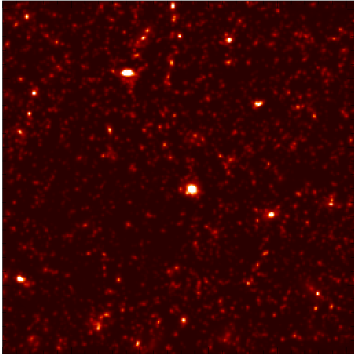
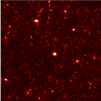
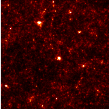
Figure 1: Convergence maps ($3^{\circ}\times 3^{\circ}$) from different selections of particles. From upper left to lower right: only particles in halos more massive than $M=10^{14}$, $10^{13}$ and $10^{12}\,h^{-1}M_{\odot}$ and finally, all particles. The maps have been smoothed with a Gaussian with FWHM$=1^{\prime}$ and the scale is between -0.036 and 0.2.

Figure 2: Convergence power spectra resulting from simulations of structure formation. We show the spectrum resulting from all structure except halos with mass above masscuts of $10^{15}\,h^{-1}M_{\odot}$ (solid), $10^{14}\,h^{-1}M_{\odot}$ (dashed) and $10^{13}\,h^{-1}M_{\odot}$ (dotted). On average, the power from halos less massive than $10^{14}\,h^{-1}M_{\odot}$ is about a factor 2 lower than the total power.

Using the simulation data and the group information of each particle, we construct convergence maps for different selections of particles. Structure that is left out this way is replaced by a uniform matter density such that all maps have the same average convergence. In Fig. 1 we show the contributions to the convergence field from halos with masses above $10^{14}$, $10^{13}$ and $10^{12}\,h^{-1}M_{\odot}$. In Fig. 2 we show the power spectra of maps where the effect of halos more massive than certain mass cuts has been taken out. The cuts are chosen to be $10^{15},10^{14}$ and $10^{13}\,h^{-1}M_{\odot}$ in order to be able to compare the results to the analytical results of Cooray, Hu & Miralda-Escude (2000). Fig. 2 shows that the power spectrum coming from matter in halos with mass below $10^{14}\,h^{-1}M_{\odot}$ and ungrouped matter is about half of the total, which agrees nicely with their predictions. The power from halos less massive than $10^{13}\,h^{-1}M_{\odot}$ and ungrouped matter is roughly 10% - 20%. Since the selection of line-of-sight halos we will be able to find in optical data will be determined by a (redshift dependent) minimum mass, very roughly corresponding to the mass cuts in Fig. 2, we already see that a significant part (in terms of the power spectrum) of the projection effect will be difficult to correct for.

3.2 Deprojecting known halos

Figure 3: Scatter in mass estimates from $\gamma_{\rm T,halo}$ with respect to the virial mass $M_{200}$ for the set of 141 target halos defined in the text. $\gamma_{\rm T,halo}$ is the shear at $r=r_{200}/2$ purely caused by the halo of interest, so line-of-sight projection has not yet been taken into account. The arrows indicate the median (left) and the mean (right). The histogram that even if we are able to correct for the projection effect of all line-of-sight structure perfectly, we still have to deal with the fact that the enclosed mass within $r$ may differ from $M_{200}$ and the fact that $\gamma_{\rm T,halo}$ does not exactly correspond to the enclosed mass if $\kappa(r)\not=0$.

Figure 4: Scatter in mass estimates based on the transverse shear for a sample of 141 massive halos defined in the text. $\gamma_{\rm T}$ is the average shear at radius $r_{200}/2$. Projection effects of line-of-sight structure cause a large scatter in mass estimates derived directly from the measured shear.

In this and the following section we investigate to what extent we can eliminate line of sight projection if we know the masses and positions of (some of) the line-of-sight halos. As a measure for the mass enclosed within a transverse radius $r$ of the halo center we use $\gamma_{\rm T}(r)$, the average tangential shear at $r$, because unlike the convergence this is a quantity that can be observed. It is related to the convergence by

$$\gamma_{\rm T}(r)=\kappa(<r)-\kappa(r)$$ (5)

(see for example Mandelbaum et al. 2004). Here $\kappa(<r)$ and $\kappa(r)$ are the average convergences within the area with radius $r$ and at $r$ respectively. The mass of a certain halo within $r$ relates to the tangential shear caused only by that halo $\gamma_{\rm T,halo}$ through:

$$M_{\rm encl}(r)\propto\frac{c^{2}}{4\pi G}\frac{\chi_{s}}{(1+z)\chi(\chi_{s}-\chi)}A_{\rm halo}\gamma_{\rm T,halo}(r),$$ (6)

where $A_{\rm halo}$ is the projected surface area of the region within $r$ in units of comoving distance squared and the relation is an equality if $r$ is big enough for $\kappa(r)$ to be zero since in that case $\gamma_{\rm T,halo}(r)=\kappa_{\rm halo}(<r)$. If $\kappa(r)>0$, we need to multiply $\gamma_{\rm T,halo}$ by a correction factor before we can relate it to the mass by the above equation. If the halo has an NFW profile with $c\approx 4$, this factor will be about $1.6$ at a radius $r=r_{200}/2$. We calculate the shear for a set of target halos defined by $M>3\times 10^{14}\,h^{-1}M_{\odot}$ and comoving distance between $500$ and $1900\,h^{-1}$Mpc, so that the lensing kernel is at least about half of its maximum. Using 10 realisations this gives us a set of 141 halos.

Figure 5: Distribution of the number of halos above mass cuts of $10^{14}\,h^{-1}M_{\odot}$ and $5\times 10^{13}$ that lie along the line of sight of a certain halo. The number of halos along the line-of-sight was calculated for a set of 141 massive halos (see text) and a halo is considered to lie on the line of sight of one of those halos if their projected separation is less than the sum of their virial radii. We will assume that line-of-sight halos more massive than the above mass thresholds can be identified in optical surveys. The histograms show that there is only a small number of these halos along the line of sight of each target halo and therefore one might expect that they account for only a small part of the line-of-sight projection.

The transverse radius $r$ the shear is evaluated at is taken to be $r_{200}/2$. The disadvantage of this choice of $r$ is that this way we do not get information about the mass of the part of the halo that lies outside of $r_{200}/2$. However, for larger radii, a lot of pixels with low signal will be included and the signal to noise ratio consequently will go down. We checked that $r=r_{200}/2$ gives shear measurements with less noise from projection than larger values of $r$. In Fig. 3 we show the relation between the virial mass and the mass enclosed within $r=r_{200}/2$ as calculated from $\gamma_{\rm T,halo}(r)$, using Eq (6) with a correction factor of $1.6$. $\gamma_{\rm T,halo}$ is obtained from the lensing field with just the halos more massive than $3\times 10^{14}\,h^{-1}M_{\odot}$ in it. Since there are only a few halos more massive than $3\times 10^{14}\,h^{-1}M_{\odot}$ in each map, this practically means that for each target halo, $\gamma_{\rm T,halo}$ is the shear purely caused by that halo. The scatter is due to the fact that the ratio of $\kappa(r)$ over $\gamma_{\rm T,halo}$ is not always exactly 1.6 and, more importantly, the fact that the mass enclosed does not in general equal $M_{200}$ (see for example Metzler, White & Loken 2001 for a more detailed discussion of this issue). The enclosed mass for example has a large dependence on the orientation of the halo in case it is elliptical. In the rest of this paper we will ignore the problem of calculating the (virial) mass in case $\gamma_{\rm T,halo}$ is known and instead focus on the problem of how to find $\gamma_{\rm T,halo}$ in the first place.

Figure 6: Scatter in mass estimates based on the transverse shear for a sample of 141 massive halos defined in the text. $\gamma_{\rm T}$ is the average shear at radius $r_{200}/2$ after correcting for the projection effect of line-of-sight halos more massive than $M_{\rm threshold}$ and $\gamma_{\rm T,halo}$ is the shear purely caused by the halo of interest. Since we completely correct for the effect of halos above the thresholds, these results show that most of the scatter is caused by halos below the mass thresholds and by unclustered matter.

In Fig. 4 we show how much the “measured” shear $\gamma_{\rm T}$, caused by all structure along the line of sight, deviates from the shear that is caused by just the halo of interest $\gamma_{\rm T,halo}$. In light of the discussion in the previous paragraph, Fig. 4 shows that projection effects will cause large errors in mass estimates obtained from the uncorrected lensing field. Fig. 5 shows the statistics of how many halos more massive than mass thresholds of $1\times 10^{14}$ and $5\times 10^{13}\,h^{-1}M_{\odot}$ there are along the line of sight of each of the target halos. We choose these particular thresholds because virtually all halos more massive than these thresholds can be detected from deep optical surveys (Gladders & Yee, 2000) while for lower thresholds this will become very difficult. We correct for the lensing effect by these line-of-sight halos by using the actual matter distribution (from the N-body simulations) of each line-of-sight halo to calculate its contribution to the lensing field and subsequently subtract this from the “measured” total field. We also include in this correction all structure within $3r_{200}$ of the halo center that is not part of the halo by our FoF halo definition described in section 2.1 because we do not want to exclude the lensing effect of structure that can be considered part of the halo but is not part of the FoF halo. In Fig. 6 we show that the scatter only gets a little smaller when we correct for the lensing field caused by halos above the thresholds. These plots provide us with an upper limit on how well we can correct for halos above the given mass thresholds. In reality, we do not know the exact profiles of the line-of-sight halos, which means we have to resort to a halo model (see section 2.2) to correct for their effect.

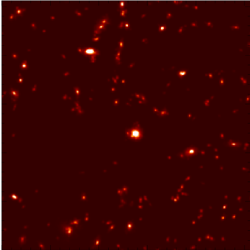
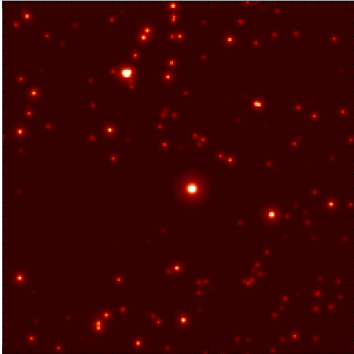
Figure 7: Convergence maps that only take into account halos more massive than $10^{14}\,h^{-1}M_{\odot}$. On the left we use the simulated matter distribution. On the right, we use the halo catalog together with our NFW halo model. We use maps of this type to correct for the lensing effect of “known” halos by subtracting them from the complete convergence maps. The maps have been smoothed with a Gaussian with FWHM$=1^{\prime}$ and the scale is between -0.036 and 0.2.

We also construct convergence maps using halo masses and positions from the halo catalog assuming all halos follow NFW density profiles. Earlier work shows that lensing maps using the NFW profile can have power spectra that agree with power spectra obtained from simulated matter distributions very well (Ma & Fry, 2000; Seljak, 2000). In Fig. 7 we show such a map only taking into account halos more massive than $10^{14}\,h^{-1}M_{\odot}$ next to the map using the original simulation data with the same mass threshold. The two lensing fields indeed look fairly similar, even though it is obvious that the assumption that halos are spherically symmetric is an idealization. We now use NFW convergence maps, only including halos above certain mass thresholds, to correct for the lensing effect of those halos (Fig. 8) by first subtracting the NFW convergence map from the complete map and then calculating the tangential shear. Comparison with the previous case where we use the exact density profile to calculate the correction shows that assuming an NFW profile introduces extra scatter.

The former results show that our ability to retrieve $\gamma_{\rm T,halo}$ is severely limited by the lensing effect of halos below the mass thresholds and mass that is not part of any halo at all. Only a small part of the scatter is caused by the halos we correct for, defined by $M>M_{\rm threshold}$. This can be explained by the fact that each target halo has only a small number of these halos along its line of sight (Fig. 5). We explicitly checked that as we go to lower mass thresholds the histograms tighten significantly, but we must reduce $M_{\rm threshold}$ to values smaller than $10^{12}\,h^{-1}M_{\odot}$ for the width to drop below 10 %. The NFW results, in addition, suffer a little from the fact that we use idealized halo shapes to calculate the correction. We expect that this situation can be improved by changing the halo model. For example, one could allow for elliptical halos instead of only spherically symmetric ones and there may also be some gain in modelling halos beyond the virial radius. We will not pursue these approaches here though. As noted before, no matter how much we improve our halo model, we will never be able to reduce the scatter further than in the case shown in Fig. 6 (unless we can find line-of-sight halos down to much lower masses).

Figure 8: Scatter in mass estimates based on the transverse shear for a sample of 141 target halos defined in the text. $\gamma_{\rm T}$ is the measured shear after correcting for the projection effect of line-of-sight halos more massive than $M_{\rm threshold}$ assuming NFW profiles for those halos. $\gamma_{\rm T,halo}$ is the shear purely caused by the halo of interest. In addition to the error caused by the projection effect from halos below the thresholds, the slight extra scatter with respect to Fig. 6 is caused by the difference between true halo shapes and the assumed NFW model.

3.3 Mass based on cluster richness

Figure 9: Scatter in mass estimates based on the transverse shear for a sample of 141 massive halos (see text). $\gamma_{\rm T}$ is the measured shear after correcting for the projection effect of line-of-sight halos more massive than $M_{\rm threshold}$ assuming NFW profiles and estimating their masses from the cluster richness. We assume our survey detects all galaxies with magnitude below $25$. $\gamma_{\rm T,halo}$ is the shear purely caused by the halo of interest. The upper plots assume all halos with $M>M_{\rm threshold}$ have been identified and in the lower plots we correct for halos with the number of observed galaxies $N>N_{\rm threshold}$.

Instead of using the catalog masses for the line-of-sight halos it is more realistic to use masses derived from an observable such as cluster richness. We expect richness data will be the most readily available mass estimator for a large sample of halos. Specifically we shall (optimistically) assume all of the dark halos above certain threshold values of the number of observed galaxies can be identified from an optical survey. We use the number of galaxies as a mass estimator. For a more detailed account on galaxies in dark matter halos, we refer to the appendix. We first use $\langle N\rangle=30(M/10^{15}\,h^{-1}M_{\odot})$ to calculate the expected number of galaxies with $L>L_{\star}(z)$, where $L_{\star}$ is defined by a corresponding absolute magnitude of $M_{\star}(z)=-20.4-z$. We then apply a random Poisson scatter to the number of satellite galaxies to get a value of $N$ for each halo. The number of observed galaxies is defined to be the number of galaxies with magnitude smaller than $25.0$ and is found using the luminosity function. The line-of-sight halo masses we use to build our NFW maps are calculated from this “observed” quantity by making the assumption $N=\langle N\rangle$ and inverting the calculations described above. The resulting masses will deviate from the real masses because of the Poisson scatter in $N-1$ and because of rounding. However, one might expect this scatter not to be so important because the average mass will not be affected and we are correcting for a number of line-of-sight halos. Another reason why the mass scatter will likely not have a big effect is that, as we saw in the previous section, the effect of halos above the thresholds is very small anyway.

We now use these masses based on cluster richness and again the assumption of NFW profiles to correct the tangential shear for projection effects. The results are shown in Fig. 9 for different selections of halos. We first consider the case where all halos above mass threshold of $1\times 10^{14}$ and $5\times 10^{13}\,h^{-1}M_{\odot}$ have been identified to compare with results from the previous section (top). As expected, the added uncertainty in mass does not make a big difference. The most realistic cases we consider are those corresponding to the results in the bottom two plots. Here, whether a halo is considered to be observable or not is based on a minimum observable galaxy number (10 and 25) instead of a minimum mass.

4 Conclusions

Gravitational lensing provides a powerful means to measure the mass distribution in the universe. We were hoping that we could use the tangential shear caused by dark matter halos to find their masses. A problem would be the effect of other mass along the line of sight on the shear. We investigated if it is possible to use positions and masses of line-of-sight halos obtained from deep field optical data to correct for this effect. In section 3.2 we showed that even if we can correct for the lensing effect of all line-of-sight halos with mass above $5\times 10^{13}\,h^{-1}M_{\odot}$ perfectly, the effect of halos below that mass and unclustered matter is big enough to make halo mass estimates based on the shear deviate strongly (20% deviations are not very rare) from the actual masses. Since in reality we will not know the exact shapes of halos, this sets a limit on how accurately we may hope to calculate individual halo masses.

This brings us to the second problem. In reality we will have to use a model for the shapes of halos. Assuming all halos follow a NFW matter distribution causes estimated contributions of line-of-sight halos to the lensing field to deviate from the actual contributions. Of course, more realistic models could improve the results, but only up to the limit mentioned above. Finally, in section 3.3 the use of galaxy counts to find the masses of line-of-sight halos has been taken into account. We conclude that it is very difficult to use the tangential shear to calculate masses of individual halos with high accuracy and it is unlikely that any other measure of the lensing field can be used for this purpose. An interesting future project would be to investigate the more statistical approach of comparing predictions of the shear (or an other observable measure of the lensing field) as a function of halo mass from simulations to measured lensing fields around a large sample of halos to find the number of halos per mass range. While it has never been demonstrated that high accuracy calibration of the shear-mass relation is possible using simulations, there is in principle no obstacle to this route. Of course, using simulations to calibrate observations, rather than test algorithms, is more demanding of the theory.

We would like to thank Chris Vale for useful discussions and also Alexandre Amblard and Joseph Hennawi for their helpful comments on an earlier draft.

5 Appendix: Galaxy counts

Generally, a halo contains $1$ central galaxy and $N-1$ satellite galaxies above a certain reference luminosity $L_{\star}$, where the number of satellite galaxies follows a Poisson distribution (Kravtsov et al., 2004). The mean number of galaxies as a function of mass is given by the relation $\langle N\rangle\sim M^{\alpha}$, with $\alpha\approx 0.9$. The number of galaxies that we will be able to observe will likely be determined by an upper limit on the apparent magnitude, which can be related to a minimum luminosity $L_{\rm min}$ if we know the physical distance to the galaxy/halo. The number of galaxies per volume in a given luminosity range is given by the Schechter luminosity function:

$$\phi(L)dL=\phi_{\star}\left[\frac{L}{L_{\star}}\right]^{\beta}e^{-L/L_{\star}}dL\ \ \ \ (\beta\approx-1),$$ (7)

from which it follows that

$$N_{L>L_{\rm min}}=N\,\frac{\Gamma(\beta+1,L_{min}/L_{\star})}{\Gamma(\beta+1,1)},$$ (8)

where $N_{L>L_{min}}$ is the number of galaxies in the halo with $L>L_{min}$, $N$ is the number of galaxies with $L>L_{\star}$ discussed above and $\Gamma(\alpha,x)$ is the incomplete gamma function. The relations above can be used to relate the number of observed galaxies to the halo mass. Of course, the accuracy of this method is limited because of the Poisson scatter in the number of satellite galaxies and because the relations used are far from exact.

References

- (1)
- Bacon (2000) Bacon D. J., Refregier A. R., Ellis R. S., 2000, MNRAS, 318, 625
- Bahcall et al. (2003) Bahcall N. A. et al., 2003, ApJ.Suppl., 148, 243-274
- Bullock et al. (2001) Bullock J. et al., 2001, MNRAS, 321, 559
- Cooray, Hu & Miralda-Escude (2000) Cooray A., Hu W., Miralda-Escude J., 2000, ApJ, 535, L9
- Davis et al. (1985) Davis M., Efstathiou G., Frenk C. S., White S. D. M., 1985, ApJ, 292, 371-394
- Dodelson (2004) Dodelson S., 2004, Phys.Rev.D70
- Eisenstein & Hu (1999) Eisenstein D. J., Hu W., 1999, ApJ, 511, 5
- Gladders & Yee (2000) Gladders M. D., Yee H. K. C., 2000 [astro-ph/0011073]
- Hennawi & Spergel (2004) Hennawi J. F., Spergel D. N., 2004, submitted to ApJ [astro-ph/0404349]
- Hoekstra et al. (2002) Hoekstra H., Yee H. K. C., Gladders M. D., Barrientos L. F., Hall P. B.,Infante L., 2002, ApJ, 572, 55
- White & Hu (2000) White M., Hu W., 2000, ApJ, 537, 1
- Jain, Seljak & White (2000) Jain B., Seljak U., White S. D. M., 2000, ApJ, 530, 547
- Jarvis et al. (2003) Jarvis M., Bernstein G., Jain B., Fischer P., Smith D., Tyson J. A.,Wittman D., 2003, AJ,125,1014
- Kravtsov et al. (2004) Kravtsov A. V. et al., 2004, ApJ, 609, 35-49
- Ma & Fry (2000) Ma C., Fry J. N., 2000, ApJ, 543, 503-513
- Mandelbaum et al. (2004) Mandelbaum R., Tasitsiomi A., Seljak U., Kravtsov A. V., Wechsler R. H., 2004 [astro-ph/0410711]
- Metzler, White & Loken (2001) Metzler C. A., White M., Loken C., 2001, ApJ, 547, 560
- Mohr (2002) Mohr J. J., 2002, Contribution to AMiBA 2001 Proceedings, ASP conference Series [astro-ph/0112502]
- Mohr et al. (2002) Mohr J. J., O’Shea B., Evrard A. E., Bialek J., Haiman Z., 2002, contribution to Dark Matter 2002 conference proceeding [astro-ph/0208102]
- Navarro, Frenk & White (1995) Navarro J. F., Frenk C. S., White S. D. M., 1995, MNRAS 275, 720
- Navarro, Frenk & White (1996) Navarro J. F., Frenk C. S., White S. D. M., 1996, ApJ, 462, 563
- Navarro, Frenk & White (1997) Navarro J. F., Frenk C. S., White S. D. M., 1997, ApJ, 490, 493
- Padmanabhan et al. (2003) Padmanabhan N., Seljak U., Pen U. I., 2003, New Astronomy, 8, 581
- Refregier (2003) Refregier A., 2003, ARA&A, 41, 645
- Rhodes et al. (2001) Rhodes J., Refregier A., Groth E. J., 2001, ApJ, 552, L85
- Seljak (2000) Seljak U., 2000, MNRAS 318, 203
- Sheth & Tormen (2001) Sheth R. K., Tormen G., 2002, MNRAS 329, 61
- Vale & White (2003) Vale C., White M., 2003, ApJ, 592, 699-709
- Wang & Steinhardt (1998) Wang L., Steinhardt P. J., 1998, ApJ, 508, 483-490
- White (2002) White M., 2002, ApJ Suppl. 143, 241
- White & Vale (2004) White M., Vale C., 2004, Astropart.Phys. 22, 19
- White, van Waerbeke & Mackey (2002) White M., van Waerbeke L., Mackey J., 2002, ApJ, 575, 640-649
- Van Waerbeke et al. (2000a) Van Waerbeke L. et al., 2000, A&A, 358, 30
- Van Waerbeke & Mellier (2003) Van Waerbeke L., Mellier Y., 2003 [astro-ph/0305089]
- Yan & White & Coil (2004) Yan R., White M., Coil A., 2004, ApJ, 607, 739-750