The Neon Abundance of Galactic Wolf–Rayet Stars

Abstract

The fast, dense winds which characterize Wolf-Rayet (WR) stars obscure their underlying cores, and complicate the verification of evolving core and nucleosynthesis models. Core evolution can be probed by measuring abundances of wind-borne nuclear processed elements, partially overcoming this limitation. Using ground-based mid-infrared spectroscopy and the 12.81$\mu m$ [Ne ii] emission line measured in four Galactic WR stars, we estimate neon abundances and compare to long-standing predictions from evolved-core models. For the WC star WR 121, this abundance is found to be $\gtrsim 11\times$ the cosmic value, in good agreement with predictions. For the three less-evolved WN stars, little neon enhancement above cosmic values is measured, as expected. We discuss the impact of clumping in WR winds on this measurement, and the promise of using metal abundance ratios to eliminate sensitivity to wind density and ionization structure.

1. INTRODUCTION

Wolf–Rayet (WR) stars are evolved massive stars characterized by high mass loss rates ($10^{-5}\leq\dot{M}\leq 10^{-4}\>\mathrm{M}_{\odot}\>\mathrm{yr}^{-1};\dot{M}_{WR}\sim 10^{10}\>\dot{M}_{\odot}$), driven in fast ($v_{\infty}\sim\mathrm{few}\times 10^{3}\,\mathrm{km/s}$) stellar winds. The dense WR winds obscure their underlying cores and the region from which the outflowing wind material is initially accelerated. The difficulty in quantifying bulk parameters of WR stars which arises due to this obscuration is typified by the uncertainty regarding the appropriate photospheric temperature to assign them. When the most commonly used definition of the photosphere is adopted (the location of optical depth $\tau\sim 2/3$), a temperature degeneracy arises in the models of WR atmospheres — for all WR subtypes, the effective photospheric temperature derived is $T_{2/3}\sim 30,000\,\mathrm{K}$, for reasons unknown (Schmutz, Leitherer, & Gruenwald, 1992). More effective for predicting luminosity and emergent flux distribution is the inferred core temperature, but this assignment depends critically on the ad hoc choice of a velocity structure of the wind, the commonly assumed form of which Schmutz (1997) showed to be largely invalid in the single WR star (HD 50896 – WR 6) for which the optically thin, supersonic portion of the wind has been modeled hydrodynamically. Testing models of WR core evolution, and the advanced nuclear reactions which occur there, is complicated by this disconnect between the observable bulk properties of the wind, and the wind-driving core buried beneath it.

A powerful technique for probing WR core evolution which sidesteps these difficulties is available in the measured abundances of wind-borne nuclear processed elements. Neon in particular undergoes a remarkable abundance change during the later stages of a WR star’s lifetime. By the end of the more evolved WC phase (characterized by wind material dominated by $\alpha$-burning by-products, carbon in particular), ${}^{22}\mathrm{Ne}$ becomes the fourth most abundant element, after ${}^{4}\mathrm{He}$, ${}^{12}\mathrm{C}$, and ${}^{16}\mathrm{O}$. The reactions of interest contributing to the creation of neon during He-burning in massive stars are (Maeder, 1983):

${}^{14}\mathrm{N}$$(\alpha,\gamma)\Rightarrow$${}^{18}\mathrm{F}$$(\beta,\nu)\Rightarrow$${}^{18}\mathrm{O}$$(\alpha,\gamma)\Rightarrow$${}^{22}\mathrm{Ne}$ $(\alpha,n)\Rightarrow$${}^{25}\mathrm{Mg}$ $(\alpha,\gamma)\Rightarrow$${}^{26}\mathrm{Mg}$

${}^{4}\mathrm{He}$$(\alpha,\gamma)\Rightarrow$${}^{8}\mathrm{Be}$$(\alpha,\gamma)\Rightarrow$${}^{12}\mathrm{C}$$(\alpha,\gamma)\Rightarrow$${}^{16}\mathrm{O}$$(\alpha,\gamma)\Rightarrow$${}^{20}\mathrm{Ne}$

Essentially all of the ${}^{14}\mathrm{N}$ produced via the CN branch of the CNO cycle which dominates the earlier WN evolutionary phase is converted to ${}^{22}\mathrm{Ne}$. The further conversion of neon to ${}^{25}\mathrm{Mg}$ and ${}^{26}\mathrm{Mg}$ is inefficient except at the highest temperatures (achieved only in stars with initial masses $\gtrsim 100\textrm{M}_{\odot}$), and the production of ${}^{20}\mathrm{Ne}$ via ${}^{16}\mathrm{O}$ is also negligible except in the most advanced WC and WO stages of the highest mass stars. The two main consequences of these critical neon production chains are a strong increase in the overall abundance of neon by a factor of $\sim$200 over the course of the WR phase, and a rise in the isotopic abundance ratio ${}^{22}\mathrm{Ne}$/${}^{20}\mathrm{Ne}$ from $\sim$0.1 to $\sim$35. Both of these changes to the neon abundance occur quite rapidly (in the course of several thousand years) at the onset of the WC phase. Late-stage depletion of ${}^{22}\mathrm{Ne}$ by conversion to magnesium is only 30% during the final $10^{6}$ yr of the most massive stars’ lives, with the overwhelming majority of WRs maintaining their full neon excess, thanks to the combined effects of the interior mixing and mass-loss which bring material to the surface. Assuming normal p-p nuclear processing of hydrogen entirely to helium, the cosmic abundance of neon by number is $\mathrm{Ne/He}=3.7\times 10^{-4}$ (see § 5.5). The neon abundance predicted by WR evolutionary models is $\mathrm{Ne/He}=6.6\times 10^{-3}$, or over 17 times the cosmic value. This result, first described by Maeder (1983), has remained valid despite recent model updates to accomodate rotational mixing and the turbulent diffusion of core material into the wind it drives (Maeder & Meynet, 2000).

We will give background on the detection of neon in WR winds in § 2, describe the observations in § 3, outline the abundance calculation and inputs in §§ 4–5, and present the results in § 6.

2. BACKGROUND

Despite lingering uncertainties concerning the true structure of WR winds, broad agreement between the surface abundances predicted by core evolution models was obtained early on for almost all abundant elements, both for WN (e.g. Crowther, Hillier, & Smith, 1995a) and WC (e.g. Maeder & Meynet, 1994) stars. However, a long standing discrepancy concerning the model-sensitive neon abundance predictions centered on $\gamma^{2}$ Velorum (WC8), the nearby, optically-brightest WR star. While the Maeder abundances were well-confirmed for all other elements, the measured neon abundances of $\gamma^{2}$ Vel remained quite low, near or just above the cosmic value.

In one of the earliest mid-infrared (MIR) measurements of a WR star, Aitken, Roche, & Allen (1982) calculated Ne⁺ and S³⁺ abundances in $\gamma^{2}$ Vel from ground-based spectra. van der Hucht & Olnon (1985) found a similarly elevated neon abundance for $\gamma^{2}$ Vel using IRAS LWS spectra, seemingly confirming its predicted over-abundance with respect to cosmic levels. Both of these results, however, were later significantly corrected by Barlow et al. (1988), who discovered flaws in the calculations and in the atomic inputs, and found a revised neon abundance again quite close to cosmic values. Dessart et al. (2000) adjusted $\gamma^{2}$ Velorum’s neon abundance yet again, using ISO data and an improved distance value along with more modern, clumping-corrected mass loss rates to derive a value coincidentally quite close to the original determination of Aitken et al., and in good agreement with theory. Willis et al. (1997) found an elevated neon abundance in the ISO SWS spectrum of WR 146 (WC5), and in total, four ISO WC stars (Willis et al., 1997; Dessart et al., 2000) and one WN star (Morris et al., 2000) have yielded neon abundances. Morris et al. (2004) used early Spitzer IRS spectra to measure the neon abundance of WN4 star WR6, and found values consistent with no enhancement.

Table 1Program WR Stars with Observed Neon

Object	Name	Spectral	D	$A_{v}$		$v$	$f_{10\mu m}$
		Type	(kpc)	(mag)		(mag)	(Jy)
WR 105	Ve2-47	WN9h	1.58	8.63 $\pm$	.03	12.92	0.68
WR 116	ST 1	WN8h	2.48	6.89		13.38	0.44
WR 121	AS 320	WC9d	1.83	5.72 $\pm$	.32	12.41	1.51
WR 124	209 BAC	WN8h	3.36	4.43		11.58	0.14

Note. — All spectral types, magnitudes, and extinction coefficients are from van der Hucht (2001). Extinctions with quoted errors are for stars with known cluster associations, and are considerably more accurate.

3. OBSERVATIONS

Smith & Houck (2001) (hereafter SH01) present a flux-calibrated 8–13 µm spectral survey of a large sample of northern Galactic WR stars representing all sub-types. Among the sample, four stars exhibited broad, non-nebular [Ne ii] 12.81 µm line emission. These are listed in Table 1, along with spectral types, photometric or cluster distances and reddening, visual magnitudes and mid-infrared fluxes. The spectra were obtained with Score (Smith et al., 1998; Van Cleve et al., 1998), a prototype instrument for the short wavelength, high resolution module of Spitzer’s IRS spectrograph (Houck et al., 2004), operated at the Palomar 5m. Standard beam-switched 5Hz chopping and nodding were used to remove the sky signal. The chop amplitude was chosen to be small enough so that the object fell within Score’s 12″ diameter slit-viewer field when the slit was on adjacent sky. Two equal amplitude source images in the slit-viewer’s 11.3 µm silicate filter were thus obtained simultaneously with the spectra, and used to correct the absolute flux calibration for the changing slit throughput function, which is affected by seeing, pointing accuracy, and object acquisition. This calibration, and a general description of the spectral reduction process, are described in more detail by SH01. Initial flux-calibration was performed using same-airmass observations of Cohen et al. (1995) infrared standard stars. Line strengths were computed using a polynomial fit to the nearby continuum. Fig. 1 shows the Score MIR spectra of one of the WN and the single WC program stars. The WN star exhibits lines of helium and neon, while the WC star exhibits only [Ne ii].

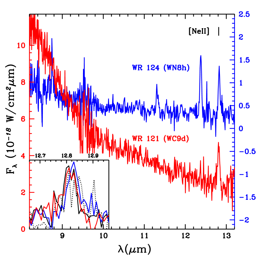
Figure 1.— Score spectra of two of the program stars. The [Ne ii] 12.81 µm line is inset for all four stars (solid: WR105, dotted: WR116, see SH01 for full spectra). The dusty WC9d has a steep slope typical of $\sim$1000K heated dust emission, with a slight break in the slope at 9.5 µm, characteristic of moderate, broad silicate absorption. The noise excess in both spectra at 9.7 µm is due to telluric O₃.

One distinct difference between the Score data used here and ISO SWS spectra used to compute previous neon abundances is worth mentioning. The entirety of ISO’s SWS spectral beam ($\sim 20\arcsec\times 35\arcsec$) is mapped onto the spectrograph’s large detector elements and is included in the recorded spectra. For this reason, contamination by nebular emission lines originating in the often bright, extended nebulae surrounding WR stars is often a concern. Score’s small $1\arcsec\times 2\arcsec$ slit excludes most of this nebular emission, leading in some cases to significant differences between spectra of the same non-variable WR star observed with both ISO and Score (cf. WR146 in Willis et al. (1997) vs. SH01, as described in §4.2 of the latter). While we know of no cases in which neon or other abundances computed using ISO data were affected by this type of contamination, the Score spectra of fainter WR stars used here should be relatively less affected by nebular emission.

4. CALCULATING NEON ABUNDANCE

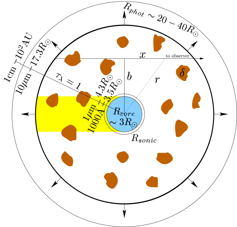
Figure 2.— Wind model geometry. Observer is to the right, along the line of sight coordinate $x$. The clumps of fill factor $\delta$ are indicated schematically. The shading to the left of the core along the line of sight indicates the region from which no continuum emission is observed. Also indicated are representative physical radii for the core, sonic point, and the photosphere (from Heger & Langer, 1996), as well as the location of the continuum optical depth $\tau_{\lambda}=1$ at a variety of wavelengths, from the WN5 wind model of Hillier (1987).

4.1. Mass Loss & Clumping

For a uniform, spherical, but clumped wind with terminal velocity $v_{\infty}$ and constant volume filling fraction $\delta$ ($0\leq\delta\leq 1$), as depicted in Fig. 2, the mass loss rate can be written:

$$\dot{M}=4\pi r^{2}\delta\cdot\!n\mu m_{H}v_{\infty}$$ (1)

where $\mu$ is the mean atomic mass per ion, and $n$ is the number density of the ionized gas. Defining the standard mass loss coefficient $\mathcal{A}\equiv\frac{\dot{M}}{4\pi\mu m_{H}v_{\infty}}$, the density can be expressed as:

$$n=\frac{\mathcal{A}}{\delta r^{2}}$$ (2)

The dominant radiative output of the wind at mid-infrared and longer wavelengths is free-free emission (Wright & Barlow, 1975). The free-free optical depth along a particular line of sight through the clumped wind to the observer is

$$\tau(b)=\int\delta\kappa_{ff}dx=\delta\mathcal{K}(\nu,T)\int n_{e}n\,dx=\frac{\pi\mathcal{K}(\nu,T)\mathcal{A}^{2}\gamma_{e}}{2\delta b^{3}}$$ (3)

where the reduced free-free opacity $\mathcal{K}(\nu,T)=\kappa_{ff}/nn_{e}$, $\gamma_{e}$ is the number of electrons per ion, and we have made use of the $1/r^{2}$ density profile of Eq. 2. Assuming a constant, thermal source function, and integrating over cylinders of constant impact parameter $b$ (and thus constant free-free optical depth), we recover Wright & Barlow’s infrared/radio free-free flux expression, modified to include the effects of clumping via the fill factor $\delta$:

$$S_{\nu}=\left(\frac{\dot{M}Z}{\sqrt{\delta}\mu v_{\infty}}\right)^{4/3}\frac{\left(\gamma_{e}g_{\nu}\nu\right)^{2/3}}{D^{2}}\left(\frac{\pi e^{6}}{6\sqrt{3}c^{4}m_{H}^{2}m_{e}^{3/2}}\right)^{2/3}\Gamma(\text@frac{1}{3})$$ (4)

where $D$ is the distance to the star, $g_{\nu}$ is the frequency dependent free-free Gaunt factor, and $Z$ is the rms average charge per ion. Most WR mass loss rate estimates are derived from radio measurements of the free-free emission using Eq. 4. Given the same assumptions of atomic parameters of the wind ($Z$, $\mu$, $\gamma_{e}$), it is apparent that, in the absence of information about the clumping fill factor $\delta$, the clumping-scaled mass loss rate, $\dot{M}_{scl}\equiv\dot{M}/\sqrt{\delta}$, is derived.

4.2. Two level emission

For fine structure lines arising from ions with ground states consisting of only two energy levels, the fractional abundance of the ion by number, $\gamma_{i}\equiv n_{i}/\sum_{j}n_{j}$, can be calculated straightforwardly from the observed line flux by neglecting all other transitions. Following Barlow et al. (1988), the flux due to a given line transition can be written:

$$4\pi D^{2}\mathcal{F}_{ul}=\int\limits_{0}^{\infty}n_{u}A_{ul}h\nu_{ul}4\pi r^{2}dr$$ (5)

where $A_{ul}$ is the Einstein emission coefficient for the line in question, and $n_{u}$ is the density of the ions populating the upper level of the transition.

The upper level density and electron density follow from the definition of $\gamma_{i}$:

$$n_{u}=\frac{f_{u}\gamma_{i}\mathcal{A}}{\delta r^{2}}\>;\>n_{e}=\frac{\gamma_{e}\mathcal{A}}{\delta r^{2}}$$ (6)

where $f_{u}$ is the fraction of that ionic species present in the upper level. Plugging into Eq. 5 for $n_{u}$, we find the line flux to be:

$$\mathcal{F}_{ul}=\frac{\gamma_{i}\mathcal{A}A_{ul}h\nu_{ul}}{D^{2}}\int\limits_{0}^{\infty}f_{u}(n_{e}(r),T)\>dr$$ (7)

To derive the upper-level fraction $f_{u}(n_{e}(r),T)$, we begin with the total collisional de-excitation rate per unit volume is (Osterbrock, 1974):

$$n_{e}n_{u}q_{ul}=\sqrt{\frac{2\pi}{kT}}\frac{\hbar^{2}}{m^{\frac{3}{2}}}\frac{\Omega_{ul}(T)n_{e}n_{u}}{\omega_{u}}$$ (8)

where $\Omega_{ul}(T)$ is the collision strength, and $\omega_{u}$ is the statistical weight of the upper level. The collisional excitation rate can be obtained from the de-excitation rate using detailed balance:

$$n_{e}n_{l}q_{lu}=\sqrt{\frac{2\pi}{kT}}\frac{\hbar^{2}}{m^{\frac{3}{2}}}\frac{\Omega_{lu}(T)n_{e}n_{l}}{\omega_{l}}e^{\frac{-h\nu_{ul}}{kT}}$$ (9)

In the simple two level ion, statistical equilibrium between the levels can be written succinctly:

$$n_{e}n_{l}q_{lu}=n_{e}n_{u}q_{ul}+A_{ul}n_{u}$$ (10)

from which the upper level population can be found simply, using $n_{i}=n_{u}+n_{l}$, as

$$f_{u}=\left(1+\frac{1+\frac{n_{c}}{n_{e}}}{\frac{q_{lu}}{q_{ul}}}\right)^{-1}$$ (11)

where $n_{c}\equiv\frac{A_{ul}}{q_{ul}}$ is the critical density in the two level approximation. Plugging in for $n_{e}$ from Eq. 6, and the ratio of the collisional rates from Eqs. 8 – 9, we find

$$\mathcal{F}_{ul}=\frac{\gamma_{i}\mathcal{A}A_{ul}h\nu_{ul}}{D^{2}}\int\limits_{0}^{\infty}\left(1+\left[1+\frac{n_{c}\delta r^{2}}{\gamma_{e}\mathcal{A}}\right]\frac{\omega_{l}}{\omega_{u}}e^{\frac{h\nu}{kT}}\right)^{-1}dr$$ (12)

from which we can solve for the fractional abundance by number of the ion contributing to the line emission:

$$\gamma_{i}=\frac{2\mathcal{F}_{ul}D^{2}}{\pi\mathcal{A}^{\frac{3}{2}}A_{ul}h\nu}\frac{\omega_{l}}{\omega_{u}}e^{\frac{h\nu}{kT}}\sqrt{\frac{\delta n_{c}}{\gamma_{e}}\left[\frac{\omega_{u}}{\omega_{l}}e^{-\frac{h\nu}{kT}}+1\right]}$$ (13)

Notice that $\gamma_{i}\propto\sqrt{\delta}/\mathcal{A}^{\frac{3}{2}}$. In the absence of information about the clumping fill factor $\delta$, the scaled mass loss rate is derived from radio continuum measurements (see § 4.1). If the scaled mass loss rate is known then $\mathcal{A}\propto\dot{M}=\dot{M}_{scl}\sqrt{\delta}$, and the weak scaling of fractional abundance with clumping factor becomes $\gamma_{i}\propto\delta^{-\frac{1}{4}}$.

Note that we differ from Dessart et al. (2000) and Morris et al. (2000), who perform a numerical integration over the upper level ionic fraction $f_{u}$, after transforming from radial to density coordinates to mitigate finite step size inaccuracies near the origin. While they find discrepancies of order 20% between their analytical integral analogous to Eq. 12 and their numerical integration, we find no reason that such differences should occur for this two-level transition (for which the upper level fraction integral is exact) and presume it must have arisen from different atomic data inputs in the statistical equilibrium code used, or the finite numerical resolution of the integration.

Typically, WR wind abundances are formulated with respect to helium, almost always the most abundant element in all but the least evolved, late-type WN winds. Given knowledge of other elemental abundances, this can be calculated according to:

$$\mathrm{\frac{X_{i}}{He}}=\gamma_{i}\mathrm{\left(1+\frac{H}{He}+\frac{C}{He}+\frac{N}{He}+\frac{O}{He}+\ldots\right)}$$ (14)

where $\mathrm{X}_{i}$ represents the ion $i$, and the standard shorthand $\mathrm{X/Y}\equiv\mathrm{N_{X}/N_{Y}}$ has been used. Only the most important additional elements beyond helium are shown, and in many cases, the abundances of most will be so low that only one other element besides helium need be considered (e.g. carbon for WC stars, nitrogen and/or hydrogen for WN stars).

5. INPUTS

Table 2Atomic Data for Neon and Sulfur Lines.

Ion	Transition	Wavelength	$\omega_{l}$	$\omega_{u}$	$\Omega_{ul}$	$A_{ul}$	$n_{c}(8000\mathrm{K})$
		($\mu$m)				($10^{-3}\,\mathrm{s}^{-1}$)	($cm^{-3}$)
[S iv]	${}^{2}\!P^{\circ}_{3/2}\rightarrow{}^{2}\!P^{\circ}_{1/2}$	10.5105	2	4	8.47	7.70	3.77$\times 10^{4}$
[Ne ii]	${}^{2}\!P^{\circ}_{1/2}\rightarrow{}^{2}\!P^{\circ}_{3/2}$	12.8136	4	2	0.28	8.59	6.36$\times 10^{5}$

Note. — $\Omega_{ul}$ computed at $T_{e}=8000\mathrm{K}$. Dessart et al. (2000).

The fractional ionic abundance can be calculated directly from Eq. 13, given estimates of the distance, atomic wind parameters, and reddening. Table 2 lists the atomic data used for the two fine-structure lines considered here. The measured neon and sulfur line fluxes used here differ slightly from those presented in SH01, though the reduced spectra are unchanged. This is a result of better estimation of the continuum.

5.1. Chemical Composition

The adopted chemical composition of the winds serves only to normalize the computed abundance with respect to helium (Eq. 14), but does not change the results otherwise. All abundances mentioned are by number.

The three WN stars with neon present are all late types — the only WR type with any significant hydrogen remaining. The abundances assumed follow Nugis, Crowther, & Willis (1998), with N/He=0.005 for all late WN’s. The hydrogen content (H/He) of WR 105 (2.3) and WR 124 (1.9) were available from Nugis & Lamers (2000), computed using optical He i, He ii and H i line measurements. The latter value is also adopted for the WN8h star WR 116.

For the carbon star WR 121, the weighted mean in Nugis & Lamers for subtypes WC8-9 of carbon abundance (C/He=0.18), as well as oxygen abundance (O/C=0.2) was used. The WC9’s hydrogen abundance was assumed to be zero.

5.2. Mass Loss and Terminal Velocity

The mass loss rate enters Eq. 13 through the mass loss coefficient as $\mathcal{A}^{3/2}$, and hence significantly affects the values obtained for the abundance. Unfortunately, rates derived for individual stars often differ substantially, depending on the input assumptions, and details of the measurement. Along with imprecise distance estimates, poorly-constrained mass loss rates introduce the largest uncertainties in the computed abundances.

Eq. 4 can be used to determine the mass loss rate (or at least the scaled rate — $\dot{M}/\sqrt{\delta}$) from the measured radio flux, given independent estimates of the distance, terminal expansion velocity, and atomic parameters of the wind (e.g. Leitherer et al., 1995, 1997). The radio emitting regime is quite far out in the wind, such that the assumption that the terminal velocity has been obtained is always valid. The infrared free-free continuum, however, may not be optically thick (recall that $\kappa_{ff}\propto\lambda^{3}$ in the long wavelength limit). Contributions to the 10 µm continuum from the underlying stellar photosphere are typically only 10% of the free-free wind continuum (Barlow et al., 1981), and the cross-over from photosphere to wind-dominated emission occurs near 1–5 µm; however, since the free-free opacity is lower, the infrared emission originates deeper in the wind, sampling outflow which may not yet have reached terminal velocity, such that the assumption leading to Eq. 2 and a $1/r^{2}$ density distribution is violated, and the spectral index steepens compared to the constant velocity limit. In the absence of a valid velocity law, one possible technique to measure the mass loss rate is to scale the infrared flux with an empirically determined spectral index $\alpha$ ($f_{\nu}\propto\nu^{\alpha}$), as Barlow et al. (1981) did for $\gamma$ Velorum and HD 192163 to estimate a scaling with $\alpha=0.76$. More recently, Crowther et al. (1995a) found a value in close agreement, $\alpha=0.74$, based on a tailored analysis of several WN stars.

Scaling our MIR fluxes with this method and spectral index $\alpha=0.74$, mass loss rates for the three program WN stars (i.e. those without clear evidence of dust emission) were calculated. Each spectrum was dereddened using a composite extinction curve of Cohen (priv. communication), which, longward of $4.7\,\micron$, joins smoothly the curves used by Cohen (1993). The small inferred MIR reddening corrections are relatively uncertain, but the largest uncertainty is for the dusty types not considered in this calculation.

A 0.2 µm wide region centered on 12 µm was averaged to arrive at the Score flux density. IRAS Point Source Catalog 12 µm flux densities (Cohen, 1995) were found to be 2–5$\times$ higher, likely due to the very large IRAS beamsize. The extrapolation of the de-reddened 12 µm fluxes was performed to 4.80 GHz (6.25 cm) for comparability with Leitherer et al. (1997). Atomic parameters of the wind were adopted from Leitherer et al., using the usual relation for mean ionic mass

$$\mu=\frac{\sum\gamma_{i}m_{i}}{\sum\gamma_{i}}$$ (15)

where $m_{i}$ is the atomic mass of the ion. Only H, He, and C are included, since O never reaches abundances which would influence $\mu$ significantly. The mean molecular weights per ion Leitherer et al. compute are consistent enough within subtypes that we adopt $\mu=2.0$ for WN types later than WN6.

The mean number of electrons per ion, $\gamma_{e}$, and the RMS ionic charge, $Z$, were computed assuming He⁺ is the most prevalent ion in the radio emitting region. These quantities are very insensitive to any other assumption, since singly ionized helium and hydrogen contribute to both equivalently. Carbon is often assumed to exist as C⁺⁺ in the radio regime, but it does not significantly impact the calculation of either $\gamma_{e}$ or $Z$, each of which typically only ranges from 1.0–1.2. Given the magnitude of other uncertainties in the calculations, we adopt $Z=\gamma_{e}=1.1$. The Gaunt factor, which enters Eq. 4 through the free-free opacity, depends logarithmically on temperature and ionic charge at 4.90 GHz . We again follow Leitherer et al. in adopting $g_{4.8}=5.0$, which they computed for $T_{e}=10,000\,\mathrm{K}$.

Table 3Example Mass-Loss Rates from Various Methods.

Method	$\log(\dot{M})\>(\mathrm{M_{\odot}/yr})$		Reference
WR 105 (WN9h)
Radio	$<$-4.	41	(1)
Radio+Clumping	-4.	55	(2)
Extrapolated IR	-4.	95	(4)
Optical+1 µm Line Analysis	-4.	1	(5)
Optical+UV Line Analysis	-4.	2	(6)
WR 124 (WN8h)
Optical Line+Clumping	-4.	61	(2)
Extrapolated IR	-4.	7	(3)
Extrapolated IR	-4.	95	(4)
Optical+UV Line Analysis	-3.	8	(6)

References. — (1) Leitherer et al. (1997). (2) Nugis & Lamers (2000). (3) Barlow et al. (1981). (4) this work. (5) Schmutz, Hamann, & Wessolowski (1989). (6) Hamann & Koesterke (1998)

For two of the sources, mass loss rates were available from the clumping-corrected emission line-fitting results of Nugis & Lamers (2000): $\log(\dot{M})=-4.55$ (WR 105) and $\log(\dot{M})=-4.61$ (WR 124). Illustrating the uncertainty in the rates, Table 5.2 lists different estimates based on different techniques for two of the WN program stars. Rates based on UV, optical, IR, and radio data, with and without clumping accounted for, are listed for two of our program stars. It should be pointed out that only the Radio and Extrapolated IR methods do not require detailed modeling with the implicit ad hoc assumption for the form of the velocity field, although the IR rates do depend sensitively on the measured spectral slope for extrapolation. The variance among the different estimates is quite large, and, in the case of WR 124, the smallest and largest rates found differ by a factor of $\sim$14.

WR 105 is a confirmed non-thermal emitter (Chapman et al., 1999), with a spectral index $\alpha=-0.3$ over the 3–6 cm radio band. Since the infrared flux will likely not be modified by the thermal X-ray and non-thermal radio emission arising in the binary wind-wind collisional shocks thought to underly non-thermal WR sources (Eichler & Usov, 1993), we expect this star’s 12 µm extrapolated mass loss rate ($\log(\dot{M})=-4.95$) to be more accurate than radio-based results, and adopt it for abundance calculations.

Where available, we have preferred the radio and extrapolated infrared rates over others. In one case (WR 116) no radio or clumping corrected results were available, and we therefore adopted $\log(\dot{M})=-4.6$, based on observations of other WN8 stars.

Leitherer et al. (1997) put an upper limit on the mass loss rate of WR 121 from Australia Telescope Compact Array radio non-detection of $\log(\dot{M})<-4.5$, and Bieging et al. (1982) find a similar limit ($<$-4.55) using the Very Large Array. Abbott et al. (1986), however, had previously placed a firmer limit of $\log(\dot{M})<-4.8$. We adopt $\log(\dot{M})=-4.9$, based on values derived from radio detections of other WC9 stars, and in line with the lower mass-loss rate WC9’s exhibit compared to earlier WCs (Leitherer et al., 1997). The rate inferred from scaling WR 121’s MIR flux is not valid, having been unduly influenced by the excess heated dust emission evident in WR 121’s spectrum.

All terminal velocities are from van der Hucht (2001), except for WR 105, for which we adopt the value of Eenens & Williams (1994), $v_{\infty}=1200\,\mathrm{km/s}$, which closely matches our measurements of the [S iv] 10.5 µm FWHM in our spectrum, but deviates from most the recently cataloged value of $700\,\mathrm{km/s}$.

5.3. Temperature and Atomic Parameters

Despite the very high inferred effective temperatures ($>$60 kK) of the underlying star, WR winds are quite efficiently cooled by line radiation to $T_{e}\lesssim 10\mathrm{kK}$ in the radio emitting regime (Hillier, 1989). Though the exact temperature in the line-emitting region is uncertain, the temperature dependence of the derived ionic abundance is extremely weak at these long wavelengths ($h\nu/kT_{e}\sim.1\Rightarrow\gamma_{i}\propto T_{e}^{0.07}$); we therefore assume $T_{e}=8000\mathrm{K}$ for all four sources.

The mean ionic masses ($\mu$) and mean number of electrons per ion ($\gamma_{e}$) were taken from Leitherer et al. (1997) in the case of WR 105 and WR 121. For WR 124, $\mu$ was computed directly from the abundance ratios $\mathrm{N_{H}/N_{He}}$, and $\mathrm{N_{Z}/N_{He}}$ of Nugis & Lamers (2000). This same value was used for the other WN8h star considered, WR 116, and in both cases $\gamma_{e}=1.1$ was assumed from analogy with other late WN’s.

5.4. Total Neon Abundance

Estimating the total neon abundance from the spectra is difficult, especially since the [Ne iii] line at 15.56 µm is outside of the N-Band atmospheric window, and thus cannot be used to probe the gas in a higher ionization state. Theoretical neon ionization structure predictions could in principle be used to infer total neon abundances. Neon is now routinely included in the blanketed, non-LTE WR atmosphere code CMFGEN (Hillier & Miller, 1998), and hence its ionization structure can be modeled. It is an impurity species, and generally only has a small effect on the spectral energy distribution; it can, however, help drive the wind, especially in the outermost regions. Although a wind model specific to the very late WC9 star WR 121 was not available, by analogy to other models for low ionization WR stars (e.g. WN10), $\mathrm{Ne^{+}}$ is likely to be the dominant ion in the outer wind (J. Hillier, 2004, private communication).

Some handle on the most likely ionization state can also be had by noting that the ionization potential of S³⁺ is 35 eV, vs. $\mathrm{Ne^{+}}$: 21.6 eV and $\mathrm{Ne^{++}}$: 41.0 eV. Since their critical densities are reasonably close at these temperatures ($n_{e}\sim 10^{5}$), it is expected that the detection of [S iv] at 10.5 µm is an excellent predictor of [Ne iii]. Indeed, in the hot WN8 star WR 147, Morris et al. (2000) found [Ne iii] and [S iv], but no [Ne ii], and non-LTE model predictions of the outer winds of late WC stars show Ne⁺ as the dominant ion species (Willis et al., 1997). While the presence of [S iv] clearly does not imply a dearth of Ne⁺ (cf. WR 105, SH01, ), its absence places a stronger limit on the possible existence of Ne⁺⁺. By this argument Ne⁺ accounts for nearly all the neon in those stars with no [S iv] detection. Additional support for this conculsion as it pertains to WR 121 is provided by another WC9 star recently observed with the Spitzer’s IRS spectrograph, which offers similar resolution as Score but covers 10–40 µm. The IRS spectrum shows strong [Ne ii] without any detectable 15.56 µm [Ne iii]. This and other early IRS WR results will be presented in a forthcoming paper.

5.5. Cosmic Neon Abundance

The “cosmic” abundance of neon measured from solar coronal lines has been revised many times over the past 30 years. Recommended values for the fractional abundance by number, $\epsilon_{Ne}=10^{12}\times\mathrm{N_{Ne}/N_{H}}$ have ranged from $\log(\epsilon_{\mathrm{Ne}})=7.64$ to $8.04$ (converted from the total mass abundance of, e.g., Cameron (1973) and the references in Maeder (1983)). More recent values include those suggested by Grevesse & Sauval (1998) ($\log(\epsilon_{Ne})=8.08$), and the value found from the updated oxygen abundances of Asplund et al. (2004) ($\log(\epsilon_{Ne})=7.84$).

For evolved WC stars, the cosmic abundance is of little interest, since the bulk of the neon atoms entrained in the wind material were created directly from helium burning in the core. Final neon abundances with respect to helium can then be compared directly to model predictions, with little sensitivity on the initial amount of neon.

The less evolved WN stars do not produce any neon directly, and are therefore expected to exhibit $\mathrm{Ne/He}$ matching cosmic abundances. However, all WR stars produce, and potentially consume, helium, so that the “cosmic” value of $\mathrm{Ne/He}$ actually varies, depending on what assumptions are used to correct the helium abundance for its enhancement and/or depletion via nuclear processing. For example, Morris et al. (2000) and Morris et al. (2004) derive a corrected $\mathrm{Ne/He}$ abundance by assuming complete conversion from $4H\rightarrow He$ for the WN targets considered:

$$\left(\frac{\mathrm{Ne}}{\mathrm{He}}\right)_{corr}=\mathrm{\frac{N_{Ne}}{N_{He}+N_{H}/4}=\frac{Ne/H}{He/H+1/4}}$$ (16)

Using the latest Asplund et al. abundances, this yields a cosmic abundance $\mathrm{Ne/He}=2\times 10^{-4}$ in the severely H-depleted environment of WN winds. Barlow et al. (1988) perform a similar adjustment for the WC8 star $\gamma^{2}$ Velorum, assuming C/He=0.2 to correct $\mathrm{Ne/He}$ for processing of all hydrogen to helium, and subsequent conversion of helium to further elements.

Since any unprocessed hydrogen in the core or wind material (common in late WN stars) will invalidate the complete conversion assumption of Eq. 16, we adopt a range of cosmic $\mathrm{Ne/He}$ using the updated solar abundances of Asplund et al. (2004), from $\mathrm{Ne/He}=2.0\times 10^{-4}$ (complete H processing) to $3.7\times 10^{-4}$ (no H processing).

6. RESULTS

Table 4Neon and Sulfur Abundances.

Object	Type	$D$	$\gamma_{e}$	$\mu$	$v_{\infty}$	$\log(\dot{M})$	Line Flux	$\mathrm{\frac{X_{i}}{He}}$
		(kpc)			(km/s)	($\mathrm{M_{\odot}/yr}$)	($10^{-19}\>\mathrm{W/cm^{2}}$)	($\times 10^{-4}$)
Ne+
WR 105	WN9h	1.58	1.0	2.6	1200	-4.55	1.5	8.8
WR 116	WN8h	2.48	1.1	2.0	800	-4.6	1.6	5.3
WR 121	WC9d	1.83	1.1	4.7	1100	-4.9	2.1	41
WR 124	WN8h	3.36	1.1	2.0	710	-4.61	0.5	4.2
S3+
WR 105	WN9h	1.58	1.0	2.6	1200	-4.55	1.2	0.5

A summary of the inputs and results of the neon and sulfur abundance calculations for the four program sources are given in Table 4. Immediately apparent is the overabundance of Ne⁺ in WR 121, the late WC star. The three WN stars for which Ne⁺ abundance was measured are not expected to display abundance enhancements, since the byproducts of CNO processing should dominate. All are reasonably close to the cosmic value for $\mathrm{Ne/He}$, ranging from 1.1–4.4$\times$ cosmic (the latter corresponding to the fully-processed cosmic value), with WR 105 noticeably higher than the others.

Presuming all neon is accounted for in Ne⁺, the total neon abundance can still be increased by introducing the clumping fill factor $\delta$. If $\delta=0.1$, the abundances are increased by $\sim$1.8, presuming all other background abundances are unaffected. If all abundances (including helium) scale the same with clumping factor, the abundance ratios should technically be insensitive to it, but differing emission regimes complicate this argument (see § 7.2).

Another interesting constraint is available by considering the mass loss rate dependence. If for, e.g., the nitrogen star WR 124, the Optical+UV line analysis based rate of Hamann & Koesterke (1998) ($\dot{M}=10^{-3.8}\mathrm{M}_{\odot}\,\mathrm{yr}^{-1}$) had been adopted with all other inputs unchanged, the derived abundance would drop to $\mathrm{Ne^{+}/He}=2\times 10^{-5}$, or only $\sim$5% of the cosmic neon value. Since the reactions which convert neon to magnesium occur so rarely, and at core temperature attained only at latest stages of WR evolution and for the most massive WR cores, this casts doubt on such a high mass loss measurement; once predicted wind abundances are confirmed, neon and other products of nuclear processing can be used to constrain mass loss rates in the absence of other measures.

The WC star WR 121’s neon abundance $\mathrm{Ne^{+}/He}=4.1\times 10^{-3}$, is in quite good agreement with the long-standing prediction of $\mathrm{Ne/He}=6.6\times 10^{-3}$. Though any significant abundance of Ne⁺⁺, which we could not detect, would serve to increase $\mathrm{Ne/He}$, doubly ionized neon is not expected to be abundant in this source, due to the total absence of [S iv] emission. A realistic clumping factor of $\delta=0.15$ would imply an abundance exactly equal to the predicted value.

Sulfur, though produced in the advanced oxygen burning leading up to supernovae, is not significantly enhanced by normal stellar nucleosynthesis, and exhibits no abundance increase.

7. DISCUSSION

7.1. Neon Detection Frequency

Of the 29 WR stars cataloged by SH01, only four exhibited measurable [Ne ii] emission. The absence of neon in the remaining 25 is likely due to two factors: higher typical ionization of the wind in the neon-emitting regime, and bright continuum from heated dust diluting any spectral lines which otherwise would be present.

Among the ISO WR stars with detected neon emission, only $\gamma^{2}$ Vel (WC8) showed any non-nebular [Ne ii]. The remaining WC5–WC8 and WN8 ISO spectra exhibited only [Ne iii] 15.55 µm, which is inaccessible in the ground-based Score data. That the low [Ne ii] detection frequency is a result of higher average ionization is supported by the late subtypes of the four program stars discussed here; for both WN and WC, the subtype sequence is primarily one of ionization, with early types exhibiting lines of increasingly higher ionization species. This same earlier-type, increasing ionization sequence is also found in the trends of helium line emission strengths in the MIR spectra of SH01.

The majority of WC9 stars are dust emitters, with infrared excesses 10$\times$ or more the normal free-free excess seen in non-dust producing WR stars (Williams et al., 1987). The bright infrared continuum of heated carbon dust is usually unaccompanied by line emission in the thermal IR; presumably the lines suffer so much continuum dilution they are unmeasurable. Among the 6 WC9d late-type WC’s observed by SH01, only WR 121 showed any line emission, and indeed it is the only WC9 for which any MIR line emission has ever been observed (the two neon-emission WC10 stars reported by Aitken et al. (1980) based on early low-resolution ground-based spectroscopy were later revealed be planetary and proto-planetary nebulae).

A notable star in the original MIR sample of Smith & Houck without [Ne ii] present is WR145, a WN/WC type. The rare WN/WC transition stars, eight of which are cataloged by van der Hucht (2001), exhibit spectral signatures intermediate between the WN and WC classes, and are hypothesized to represent a transitional stage between CNO-dominated hydrogen-free WN stars, and $\alpha$-burning dominated WC stars (Crowther, Smith, & Willis, 1995b). A confirmation of enhanced neon abundance in one of the transition objects would support this interpretation, but unfortunately any neon in WR145 must be present as $\mathrm{Ne^{++}}$, as expected from the strong [S iv] emission the star exhibits.

7.2. Neon/Sulfur Abundance

As pointed out by Dessart et al. (2000), the use of neon abundances as derived in the previous section to constrain true core-evolution nuclear processes is complicated by the different emitting regimes of the elements in question. Because of their comparatively small radiative $A$ coefficients, the fine structure lines originate further out in the wind than the helium emission, at densities near $10^{5}\,\mathrm{cm}^{-3}$. A dependence on precise mass loss rates and (less problematic) terminal velocities also reduces the accuracy of direct abundance measurements, especially given the tendency of clumping to modify the measured $\dot{M}$ by factors of 2–5. A method which overcomes these difficulties is available in the $\mathrm{Ne/S}$ abundance. Since both [S iv] and [Ne ii] originate in roughly the same region of the wind, the abundance ratio derived from them should be independent of details of the wind structure, and remove any attendant systematic errors in estimating the mass loss rate, distance, and bulk parameters of the star.

The He i and He ii lines blended with [S iv] 10.5 µm are known by wind ionization models to contribute only very weakly to this line in $\gamma^{2}$ Velorum ($<$15%, De Marco et al., 2000). Due to the blend of neutral and ionized helium and hydrogen lines at this location, this contamination fraction is expected to remain nearly constant with WR subtype. We have therefore reduced the measured [S iv] input flux in Table 4 by this amount.

The $\mathrm{\mathrm{S^{3+}}/He}$ abundance found for the WN9 star WR 105 is in good agreement with the cosmic value of $\mathrm{S/He}=7.5\times 10^{-5}$, and if S⁺⁺ constitutes about one-third of the sulfur, as in WR 146 (Willis et al., 1997), the total sulfur abundance comes quite close to cosmic. The neon to sulfur ratio we find is $\mathrm{Ne^{+}/S^{3+}}=15.7$, somewhat larger than the cosmic value of the full abundance ratio $\mathrm{Ne/S}=7$. If, as expected, sulfur is less completely accounted for by S³⁺ than neon is by Ne⁺, the total sulfur abundance would be increase by a larger factor than would neon (around a factor of 2), and the final implied $\mathrm{Ne/S}$ can approach the expected cosmic value, as expected in this less-evolved WN star.

8. Conclusions

We have computed neon abundances for 3 WN and 1 WC star from ground-based spectra of the [Ne ii] 12.81 µm emission line. WR 121, the WC star, shows elevated $\mathrm{Ne^{+}}$ abundance, with an estimated total neon 11.1$\times$ the cosmic value, close to the expected 17.8$\times$ increase predicted by WR core evolution models. A significant population of emitting neon ions in the $\mathrm{Ne^{++}}$ ionization level, or realistic clumping fill factors $\delta$ would each revise this value upwards by up to a factor of 2, but distance and mass-loss rate uncertainties also contribute. Though elevated neon abundances have been found in several other WC stars, this is the least-evolved star for which such enhancement has been demonstrated. The WN stars were found to have abundances close to cosmic, consistent with no nuclear neon enhancement. For the single WN star for which neon and sulfur were both observed, the $\mathrm{Ne/S}$ ratio, which is insensitive to uncertainties in the star’s bulk parameters, was found to be consistent with cosmic values, despite larger uncertainties in the total sulfur abundance.

References

- Abbott et al. (1986) Abbott, D. C., Torres, A. V., Bieging, J. H., & Churchwell, E. 1986, ApJ, 303, 239
- Aitken et al. (1980) Aitken, D. K., Barlow, M. J., Roche, P. F., & Spenser, P. M. 1980, MNRAS, 192, 679
- Aitken et al. (1982) Aitken, D. K., Roche, P. F., & Allen, D. A. 1982, MNRAS, 200, 69P
- Asplund et al. (2004) Asplund, M., Grevesse, N., Sauval, A. J., Allende Prieto, C., & Kiselman, D. 2004, A&A, 417, 751
- Barlow et al. (1988) Barlow, M. J., Roche, P. F., & Aitken, D. K. 1988, MNRAS, 232, 821
- Barlow et al. (1981) Barlow, M. J., Smith, L. J., & Willis, A. J. 1981, MNRAS, 196, 101
- Bieging et al. (1982) Bieging, J. H., Abbott, D. C., & Churchwell, E. B. 1982, ApJ, 263, 207
- Cameron (1973) Cameron, A. G. W. 1973, Space Science Reviews, 15, 121
- Chapman et al. (1999) Chapman, J. M., Leitherer, C., Koribalski, B. ., Bouter, R., & Storey, M. 1999, ApJ, 518, 890
- Cohen (1993) Cohen, M. 1993, AJ, 105, 1860
- Cohen (1995) —. 1995, ApJS, 100, 413+
- Cohen et al. (1995) Cohen, M., Witteborn, F. C., Walker, R. G., Bregman, J. D., & Wooden, D. H. 1995, AJ, 110, 275+
- Crowther et al. (1995a) Crowther, P. A., Hillier, D. J., & Smith, L. J. 1995a, A&A, 293, 403
- Crowther et al. (1995b) Crowther, P. A., Smith, L. J., & Willis, A. J. 1995b, A&A, 304, 269
- De Marco et al. (2000) De Marco, O., Schmutz, W., Crowther, P. A., Hillier, D. J., Dessart, L., de Koter, A., & Schweickhardt, J. 2000, A&A, 358, 187
- Dessart et al. (2000) Dessart, L., Crowther, P. A., John Hillier, D., Willis, A. J., Morris, P. W., & van der Hucht, K. A. 2000, MNRAS, 315, 407
- Eenens & Williams (1994) Eenens, P. R. J., & Williams, P. M. 1994, MNRAS, 269, 1082+
- Eichler & Usov (1993) Eichler, D., & Usov, V. 1993, ApJ, 402, 271
- Grevesse & Sauval (1998) Grevesse, N., & Sauval, A. J. 1998, in Solar Composition and Its Evolution – From Core to Corona, 161–+
- Hamann & Koesterke (1998) Hamann, W. ., & Koesterke, L. 1998, A&A, 333, 251
- Heger & Langer (1996) Heger, A., & Langer, N. 1996, A&A, 315, 421
- Hillier (1987) Hillier, D. J. 1987, ApJS, 63, 947
- Hillier (1989) —. 1989, ApJ, 347, 392
- Hillier & Miller (1998) Hillier, D. J., & Miller, D. L. 1998, ApJ, 496, 407+
- Houck et al. (2004) Houck, J. R., et al. 2004, ApJS, 154, 211
- Leitherer et al. (1995) Leitherer, C., Chapman, J. M., & Koribalski, B. 1995, ApJ, 450, 289+
- Leitherer et al. (1997) —. 1997, ApJ, 481, 898+
- Maeder (1983) Maeder, A. 1983, A&A, 120, 113
- Maeder & Meynet (1994) Maeder, A., & Meynet, G. 1994, A&A, 287, 803
- Maeder & Meynet (2000) —. 2000, ARA&A, 38, 143
- Morris et al. (2004) Morris, P. W., Crowther, P. A., & Houck, J. R. 2004, ApJS, 154, 413
- Morris et al. (2000) Morris, P. W., van der Hucht, K. A., Crowther, P. A., Hillier, D. J., Dessart, L., Williams, P. M., & Willis, A. J. 2000, A&A, 353, 624
- Nugis et al. (1998) Nugis, T., Crowther, P. A., & Willis, A. J. 1998, A&A, 333, 956
- Nugis & Lamers (2000) Nugis, T., & Lamers, H. J. G. L. M. 2000, A&A, 360, 227
- Osterbrock (1974) Osterbrock, D. E., ed. 1974, Astrophysics of Gaseous Nebulae (W.H. Freeman and Co.)
- Schmutz (1997) Schmutz, W. 1997, A&A, 321, 268
- Schmutz et al. (1989) Schmutz, W., Hamann, W., & Wessolowski, U. 1989, A&A, 210, 236
- Schmutz et al. (1992) Schmutz, W., Leitherer, C., & Gruenwald, R. 1992, PASP, 104, 1164
- Smith & Houck (2001) Smith, J. D. T., & Houck, J. R. 2001, AJ, 121, 2115
- Smith et al. (1998) Smith, J. D. T., et al. 1998, Proc. SPIE, 3354, 798
- Van Cleve et al. (1998) Van Cleve, J., et al. 1998, PASP, 110, 1479
- van der Hucht (2001) van der Hucht, K. A. 2001, New Astronomy Review, 45, 135
- van der Hucht & Olnon (1985) van der Hucht, K. A., & Olnon, F. M. 1985, A&A, 149, L17
- Williams et al. (1987) Williams, P. M., van der Hucht, K. A., & The, P. S. 1987, A&A, 182, 91
- Willis et al. (1997) Willis, A. J., Dessart, L., Crowther, P. A., Morris, P. W., Maeder, A., Conti, P. S., & van der Hucht, K. A. 1997, MNRAS, 290, 371
- Wright & Barlow (1975) Wright, A. E., & Barlow, M. J. 1975, MNRAS, 170, 41