Emission measure distribution in loops impulsively heated at the foot-points

Abstract

This work is prompted by the evidence of sharply peaked emission measure distributions in active stars, and by the claims of isothermal loops in solar coronal observations, at variance with the predictions of hydrostatic loop models with constant cross-section and uniform heating. We address the problem with loops heated at the foot-points. Since steady heating does not allow static loop models solutions, we explore whether pulse-heated loops can exist and appear as steady loops, on a time average. We simulate pulse-heated loops, using the Palermo-Harvard 1-D hydrodynamic code, for different initial conditions corresponding to typical coronal temperatures of stars ranging from intermediate to active ($T\sim 3$–$10\times 10^{6}$ K). We find long-lived quasi-steady solutions even for heating concentrated at the foot-points over a spatial region of the order of $\sim 1/5$ of the loop half length and broader. These solutions yield an emission measure distribution with a peak at high temperature, and the cool side of the peak is as steep as $\sim T^{5}$, in contrast to the usual $\sim T^{3/2}$ of hydrostatic models with constant cross-section and uniform heating. Such peaks are similar to those found in the emission measure distribution of active stars around $10^{7}$ K.

1. Introduction

Coronae are important in the study of solar and stellar physics for several reasons: they are good tracers of stellar activity and of dynamo phenomena; also, bright coronae identify young stars and stellar formation regions more easily than many other characteristics. Nevertheless, fundamental aspects of stellar coronae—namely the heating mechanisms that sustain the hot, confined plasma—are not well understood. Although we are not able to observe directly the heating processes at work in stellar coronae, the characteristics of the observed coronal structures can provide us with an indirect probe for the properties of the coronal heating.

The earliest spatially resolved observations of the solar corona (e.g. Vaiana et al., 1973) have already showed that the hot plasma is highly structured and confined by the magnetic field in loop structures, which are considered the basic building blocks of the coronae. Considerable effort has been devoted in the last three decades to understanding the physics of these structures of confined plasma and to develop adequate models that account for the observed properties of coronal emission. The first loop models (e.g., Rosner et al., 1978, hereafter RTV; Vesecky et al., 1979; Serio et al., 1981, hereafter S81) were flux tubes of constant cross section filled with plasma in hydrostatic equilibrium, and in energy balance under the effects of steady heating, heat flux and radiative losses, with the magnetic field only confining the plasma. These models demonstrated a wide range of validity and satisfactorily reproduced a large number of coronal X-ray and EUV observations; both solar and stellar (e.g. Rosner & Vaiana, 1977; Pallavicini et al., 1981; Giampapa et al., 1985; Landini et al., 1985; Peres et al., 1987; Reale et al., 1988; Reale, 2002; Testa et al., 2002). However TRACE and SoHO have observed loops apparently incompatible with hydrostatic equilibrium (in terms of their spatial distribution of temperature and density) though appearing as quasi-static (e.g. Brekke et al., 1997; Warren et al., 2002; Winebarger et al., 2002; Golub, 2004). Some authors claimed that these loops are heated non-uniformly and in particular at their foot-points (Aschwanden et al., 2000, 2001; Winebarger et al., 2003). On the other hand, if the heating is too localized at the foot-points, static loops should be thermally unstable, as widely discussed since the first works on modeling of loop structures, e.g. RTV, Antiochos (1979), S81, Peres et al. (1982). Recently, detailed analyses of solar observations have brought up again the question of the location of the heating release (e.g. Priest et al., 2000; Aschwanden, 2001; Reale, 2002).

In order to attempt to explain structures that apparently persist for time scales longer than the characteristic cooling time with foot-point heating models, the models must be dynamic, since static solutions with foot-point heating can be unstable. Dynamic models of this kind have been recently used in several works (e.g. Warren et al., 2002, 2003; Spadaro et al., 2003; Müller et al., 2004). For instance, Warren et al. (2003) successfully reproduced several observed characteristics with a multi-threaded model, impulsively heating loops to several million degrees and allowing them to cool to TRACE–observable temperatures ($\sim 10^{6}$ K).

The study of the stellar coronae allows us to investigate the effect of stellar parameters (effective temperature, surface gravity, rotation, chemical composition, etc) on the coronal models, developed for the Sun. On one hand, when studying stellar coronae a first approach is based on the hypothesis that the solar corona is an adequate paradigm to interpret the observations of stellar coronae. On the other hand, the assumption of the solar analogy must be validated by comparing the characteristics of solar and stellar coronae.

Recent high quality spectral observations have provided us with detailed information on the properties of stellar coronal emission. High resolution spectra obtained with, e.g., EUVE, in the EUV range, and with the new observatories Chandra and XMM-Newton in the X-ray band, allow us to diagnose the plasma conditions in a large sample of stellar coronae at different activity levels. Since stellar coronae cannot be spatially resolved by present-day telescopes, we must resort to indirect means in order to compare the properties of coronal structures among different stars and with the observed characteristics of the solar corona. The emission measure distribution vs. temperature, $EM(T)$, defined by:

$$EM(T_{i})=\int_{\Delta T_{i}}n_{e}^{2}(T)dV,$$ (1)

where $n_{e}$ is the electron density, and V is the volume filled with plasma at $T\in\Delta T_{i}$, contains substantial information about the coronal emitting plasma, mainly on its thermal structuring, and proves to be a useful diagnostic tool for comparing the coronal emission of different stars.

The global $EM(T)$ of the X-ray Sun is typically peaked at $T\sim 2$–$3\times 10^{6}$ K and the ascending cool part is characterized by a rise as $\sim T^{3/2}$ (Orlando et al., 2000; Peres et al., 2000), even though its specific properties can vary for different coronal regions and in different phases of activity. Previous studies of the solar atmosphere, mostly done in the UV band (Jordan, 1980; Brosius et al., 1996; Landi & Landini, 1997), led to analogous results. The observed dependence on temperature is well explained in terms of hydrostatic loops (Peres et al., 2001): for a standard RTV uniformly heated loop model, the $T$ and $n$ structuring of the plasma along the loop yields $EM(T)$ increasing approximately as $T^{3/2}$. Thus, for a corona of optically thin plasma, mostly confined in hydrostatic loops, this would also yield $EM(T)\propto T^{3/2}$ in the ascending part. The descending part of $EM(T)$ gives us information on the distribution of the hydrostatic loops. Therefore, in the stellar case, the analysis of the global $EM(T)$ can provide us with information on the structuring of the observed corona, and can allow us to test the hypothesis of a corona formed by static loops at different maximum temperature.

Analyses of $EM(T)$ derived from EUV and X-ray spectra of several stars have appeared in the recent literature (e.g., Sanz-Forcada et al., 2002, 2003, present extensive $EM(T)$ reconstructions from EUVE spectra of active stars), and most of them show similar features. The $EM(T)$ of active stars is typically characterized by an ascending part as $T^{\alpha}$ with $\alpha>3/2$, and up to $\sim 5$ in some cases (see e.g. Dupree et al., 1993; Griffiths & Jordan, 1998; Drake et al., 2000; Mewe et al., 2001; Sanz-Forcada et al., 2002, 2003; Argiroffi et al., 2003; Scelsi et al., 2004). Moreover, the $EM(T)$ of several active coronae shows prominent ”bumps”, i.e. large amounts of almost isothermal material (e.g. Drake, 1996; Dupree, 1996, 2002). For example, Dupree et al. (1993) used EUVE data for the giant Capella and derived an $EM(T)$ with a well defined and narrow peak at $\log(T)\sim 6.8$, and a rise much steeper than $T^{3/2}$; the analysis of X-ray Chandra spectra of Capella (Mewe et al., 2001; Argiroffi et al., 2003) has confirmed these findings. Although these results are quite controversial and are based on atomic physics parameters still under refinement, they point to an almost isothermal hot part of the corona which, if formed by loops, does not seem to be compatible with the predictions of simple static loop models with uniform cross-section.

Isothermal loops would have fundamental implications for the thermodynamics and for the heating of the magnetized plasma. In uniformly heated loops, the energy radiated by the plasma near to the foot-points (that is at $T\sim 10^{5}$) is balanced by the local heat deposition and by the heat flux from the hotter plasma further up the loop. However, for foot-point heating, the local energy deposition can supply most of the energy radiated by the cooler plasma, so that a lower heat flux (shallower temperature gradient) is needed from the hotter plasma and the $T$ profile becomes flatter. Since standard hydrostatic loop models do not allow stable solutions for heating deposition over a spatial region smaller than about $L/3$ (e.g. S81), we decided to explore the possibility of obtaining stable loops with a non-constant and thus dynamic heating.

The possibility of a corona composed of loops heated episodically, close to their foot-points, poses two basic questions:

• Under what conditions can such loops be stable for time scales much longer than the characteristic cooling time?

• If long-lived, foot-point heated loops exist, is their $EM(T)$ different from that of uniformly heated loops?

In this work we model the properties of foot-point heated coronal loops, using a 1-D hydrodynamic model. We run simulations with pulse-heating concentrated at the foot-points, and investigate the existence of long-lived solutions; we study the $EM(T)$ associated with these solutions. In particular, we investigate the existence of stable loops characterized by an $EM(T)$ with a narrow peak and a slope steeper than $T^{3/2}$, i.e. characteristic of those derived from observations of active stars. We note that, for the solar case, Cargill & Klimchuk (2004, see also , ) demonstrated that the $EM(T)$ provides a useful diagnostic for periodically heated plasma, by using a zero-dimensional model (i.e., each loop is characterized by a single, averaged, value of density and temperature) that considers nanoflare heating (Cargill, 1994).

In §2 we describe the loop modeling and the properties of the simulations. In §3 we analyze the results of the simulations. In §4 we discuss our results and their implications, and then we draw conclusions from our work.

2. Loop Model and Set of Simulations

We model the plasma confined in a single magnetic flux tube. We will discuss later how this single loop model can be useful for interpreting the overall emission from a corona.

In our model, the magnetic field has only the role of confining the plasma; thermal conduction is effective only along the magnetic field lines. The model assumes constant cross-section along the loop. In our study, the loop half length is assumed to be $L=10^{10}$ cm, as observed for relatively long loops on the Sun. We discuss below the implications of our assumptions.

We simulate coronal loops heated close to their foot-points by episodic pulses. In order to investigate the effect of some basic parameters on the solutions for the loop plasma, we have reduced the number of free parameters as much as possible. For instance, we assume identical conditions in both loop legs and, therefore the loop model is symmetric about the loop apex. Because of this symmetry, the equations for the loop plasma are solved for half of the loop only.

The simulations are long lasting to search for long-term stability, i.e. for loops settling in a state steady on average, if such solutions exist.

Table 1Parameters of the simulations.

model		Initial conditions					Heat pulses
	$L$	$T_{\rm max}$	$p_{\rm base}$	$E_{0}$	$\tau_{\rm cool}$		$\sigma$	$\langle E_{H}\rangle$	$\tau$	$t_{\rm run}$
C	1	3	1	0.45	$\sim 2200$		L/3, L/5, L/10	$E_{0}$, 4$E_{0}$	$\tau_{\rm cool}$/4, $\tau_{\rm cool}$/2	10 000
H	1	10	36	30	$\sim 1200$		L/3, L/5, L/10	$E_{0}$, 4$E_{0}$	$\tau_{\rm cool}$/4, $\tau_{\rm cool}$/2	5 000

We use the Palermo-Harvard code (Peres et al., 1982; Betta et al., 1997); a 1-D hydrodynamic code that consistently solves the time-dependent density, momentum and energy equations for the plasma confined by the magnetic field:

$$\frac{dn}{dt}=-n\frac{\partial v}{\partial s},$$ (2)

$$nm_{\rm H}\frac{dv}{dt}=-\frac{\partial p}{\partial s}+nm_{\rm H}g+\frac{\partial}{\partial s}(\mu\frac{\partial v}{\partial s}),$$ (3)

$$\frac{d\epsilon}{dt}+(p+\epsilon)\frac{\partial v}{\partial s}=E_{\rm H}-n^{2}\beta P(T)+\mu(\frac{\partial v}{\partial s})^{2}+\frac{\partial}{\partial s}(\kappa T^{5/2}\frac{\partial T}{\partial s}),$$ (4)

with $p$ and $\epsilon$ defined by:

$$p=(1+\beta)nK_{\rm B}T\hskip 28.45274pt\epsilon=\frac{3}{2}p+n\beta\chi,$$ (5)

where $n$ is the hydrogen number density; $s$ is the spatial coordinate along the loop; $v$ is the plasma velocity; $m_{\rm H}$ is the mass of hydrogen atom; $\mu$ is the effective plasma viscosity; $P(T)$ represents the radiative losses function per unit emission measure; $\beta$ is the fractional ionization, i.e. $n_{\rm e}/n_{\rm H}$; $\kappa$ is the Spitzer conductivity (Spitzer, 1962); $K_{\rm B}$ is the Boltzmann constant; and $\chi$ is the hydrogen ionization potential. $E_{\rm H}$ is an ad hoc heating function of both space and time; this is the main parameter we vary to study the characteristics of the solutions, and it will be described in detail in §2.2. The numerical code uses an adaptive spatial grid to follow adequately the evolving profiles of the physical quantities, which can vary dramatically in the transition region.

2.1. Initial Conditions

As initial conditions, we consider hydrostatic loop solutions of the S81 model with uniform heating. In particular we have selected two different solutions with maximum temperatures: $T_{\rm max}=3\cdot 10^{6}$ K and $T_{\rm max}=10^{7}$ K. The initial model atmosphere uses the Vernazza et al. (1976) model to extend the S81 static model to chromospheric temperatures (the minimum temperature is $T_{\rm min}=4.4\cdot 10^{3}$ K). Table 1 summarizes the characteristics of the initial loop conditions: maximum temperature, $T_{\rm max}$; base pressure, $p_{\rm base}$; heating per unit time and per unit volume, $E_{0}$; and the characteristic cooling time, $\tau_{\rm cool}$, according to Serio et al. (1991):

$$\tau_{\rm cool}\sim 120\frac{L_{9}}{\sqrt{T_{7}}}.$$ (6)

This parameter is important in many respects, e.g. for comparison with the time interval between heat pulses, and other parameters of the simulations as discussed below.

Note that the parameters of the loop in Table 1 satisfy the scaling laws derived from the static RTV loop model:

$$p_{\rm base}\sim\left(\frac{T_{\rm max}}{1.4\cdot 10^{3}}\right)^{3}\cdot\frac{1}{L}$$ (7)

$$E_{0}\sim 10^{5}\cdot p_{\rm base}^{1.17}L^{-0.83}.$$ (8)

Our aim is to find solutions corresponding to loops in steady state conditions over long time scales, as observed. We find that, in general, the initial conditions have little influence on the loop evolution driven by the repeated impulsive heating, and that they can be important only in a region of the parameter space at the boundary between stability and instability. In particular, the results can change if the loop is initially already hot and dense.

2.2. The Heating Function

The heating function, $E_{\rm H}(s,t)$, is assumed to be a separate function of space and time:

$$E_{\rm H}(s,t)=H_{0}\cdot g(s)\cdot f(t)$$ (9)

Amount of Energy Release

— One of our main goals is to model stellar coronae of activity levels from intermediate to high, showing features not reproduced by standard models. The characteristic plasma temperatures for such coronae range from a few million degrees up to $\gtrsim 10^{7}$ K.

The reference value for the time-averaged intensity of the heating is the energy required to heat the initial hydrostatic model ($E_{0}$ of Table 1). We run two sets of simulations choosing $H_{0}$ such that the heating, averaged in time and along the loop, $\langle E_{\rm H}\rangle$ ($=\frac{1}{V}\frac{1}{t}\int_{V}\int_{t}E_{\rm H}(s,t)dVdt$), is equal to $E_{0}$ corresponding to $T_{\rm RTV}=3\times 10^{6}$ K and $T_{\rm RTV}=10^{7}$ K respectively. We also consider higher values of the heating ($\langle E_{\rm H}\rangle=4E_{0}$) because:

• we want to check whether unstable loops become stable with stronger heating;

• foot-point heated loops are cooler than uniformly heated loops with the same total energy input; we include simulations with stronger heating to compensate for this effect.

Spatial Distribution of Heating

— The spatial distribution of the heating is described by a Gaussian function:

$$g(s)=e^{-(s-s_{0})^{2}/(2\sigma^{2})},$$ (10)

centered at the loop foot-points (i.e. $s_{0}=0$) for all the simulations.

Figure 1.— Evolution of the temperature (left) and the density (right) distributions along (half of) a loop with semilength $L=10^{10}$ cm, initial maximum temperature $T_{\rm max}=10^{7}$ K, and constantly heated at its foot-points with $\sigma=L/3$. $T$ (in K) and $n$ (in $10^{9}$ cm^-3) are plotted vs. time (in seconds) and vs. the coordinate along the loop (in units of $10^{9}$ cm). The loop top is on the left, and the 3D plots are oriented with the initial profiles toward the observer.

We assume that the heat deposition is exactly the same in both legs of the loop, thus, as mentioned above, we have symmetry about the loop apex.

The spatial extent of the heating is a fundamental parameter of our study, given our interest in the effect of the concentration of the heating on the stability and on other characteristics of the solutions. A preliminary set of runs has indicated that the boundary between stable and unstable solutions is $\sigma\sim L/5$. Therefore, we will discuss in detail the results for $\sigma=L/10,L/5,L/3$, i.e. smaller than, equal to and larger than the critical value. For $\sigma>L/3$ the solutions do not depart significantly from the static solutions.

Temporal Distribution of Heating Pulses

— Given the transient nature of the simulated heating, a natural reference point is represented by the loop models with heating that produces flare events. In these models the heating typically consists of two terms: a constant and uniform heating keeping the steady conditions of the initial loop, i.e. the steady coronal heating; and a transient much larger heating which triggers the flare. In our analysis we neglect the constant term and assume no steady coronal heating.

The heat pulses are periodic with period $\tau$, and duty cycle 10%, i.e. the heat is active only for a pulse lasting 1/10 of the period. Each heat pulse is a step function, constant when active and zero otherwise. We consider values of $\tau$ smaller than the cooling time of the loop, $\tau_{\rm cool}$, in order to prevent the loop from collapsing, but long enough to induce significant changes in the loop.

Our choice of periodic pulses, instead of a random distribution in time, allows us to limit the free parameters and to focus on the most critical ones. We have also run test cases with random heat pulses in order to check for possible differences (Testa & Peres, 2003); solutions do not differ significantly for similar pulse parameter values (i.e. average energy release and average interval between pulses). Also Peres et al. (1993) have shown that the results do not differ substantially from those obtained with random pulses with equal average repetition time and duty cycle.

The simulations are run for at least $\sim 10$ periods and a total time, $t_{\rm run}$, much longer than the cooling time, in order to be able to distinguish between stable and unstable solutions. The total times are of the order of several hours, comparable with the time coverage of actual coronal observations.

We summarize the parameters of the simulations in Table 1.

3. Results

3.1. Evolution of Solutions

We know from previous works that loops continuously heated at the foot-points are not stable, for $\sigma<\sigma_{\rm critical}$. For comparison with pulse-heated loops, we first show the results for a loop with continuous heating.

Figure 1 shows the evolution of temperature and density for a loop evolving from initial hydrostatic conditions of $T_{\rm max}\sim 10^{7}$ K, with a foot-point heating ($\sigma=L/3$) constant in time. The evolution is shown as a 3D plot, where the temperature, $T$, and the density, $n$, are plotted vs. time and vs. the coordinate, $s$, along the loop. $s=0$, corresponds to the loop base, $s=10^{10}$ cm, to the apex; the 3D plot is oriented with the initial profiles toward the observer. The figure shows that the plasma progressively cools down and condensates at the loop apex. As discussed by e.g. RTV and S81, a configuration with temperature and density inversion ($s(T_{\rm max})$, $s(n_{\rm min})$ $<L$) is thermally unstable. Despite the continuous energy release, the loop collapses on time scales only slightly longer than the characteristic cooling time.

Figure 2 and 3 show results for pulsed heating, and in particular for an unstable and a stable loop respectively, in the same format of Figure 1.

Figure 2.— Evolution of the temperature (left) and the density (right) distributions along (half of) an unstable pulse-heated loop. The heating function parameters are: $\tau=\tau_{\rm cool}/2$, $\sigma=L/10$, $\langle E_{\rm H}\rangle=4E_{0}$ (see Table 1 for their definition). The 3D plots are in the same format as in Figure 1.

The solution shown in Figure 2 is for a loop with semi-length $L=10^{10}$ cm and heating function parameters: $\tau=\tau_{\rm cool}/2$; $\sigma=L/10$; and $\langle E_{\rm H}\rangle=4E_{0}$ (see §2 or Table 1 for their definition). Initially, the solution does not depart markedly from average conditions, but after $t\sim 2\tau_{\rm cool}$ the instability develops at the loop apex, i.e. the least heated place in the loop. As the apex plasma cools slightly, the radiative losses increase. Since the apex plasma is not sustained by significant local heat deposition, it cools down even more and condenses; the increase in density and the decrease in temperature further enhances the radiative losses. Once the instability is triggered, the loop quickly collapses because the radiative losses increase for decreasing temperature and increasing density.

All the unstable cases show similar temperature and density evolution; the more concentrated the heating, the faster the instability occurs. The instability invariably starts at the apex.

Figure 3.— Evolution of the temperature (left) and the density (right) distributions for a stable pulse-heated loop. The heating function parameters are: $\tau=\tau_{\rm cool}/2$, $\sigma=L/5$, $\langle E_{\rm H}\rangle=4E_{0}$, i.e. the parameters are the same as those of the loop of Figure 2, except for $\sigma$. The 3D plots are in the same format as in Figure 1.

Figure 3 shows an example of a long-lived solution; for a more direct comparison we show the loop with the same characteristics as that shown in Figure 2, except that the spatial deposition of the heating is $\sigma=L/5$ instead of $L/10$ (Figure 2). In spite of the fluctuations due to the heat pulses, the loop is stable on long time scales and settles to a state of higher density because of the significant chromospheric evaporation driven by the heat pulses.

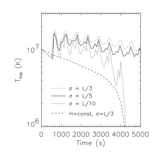
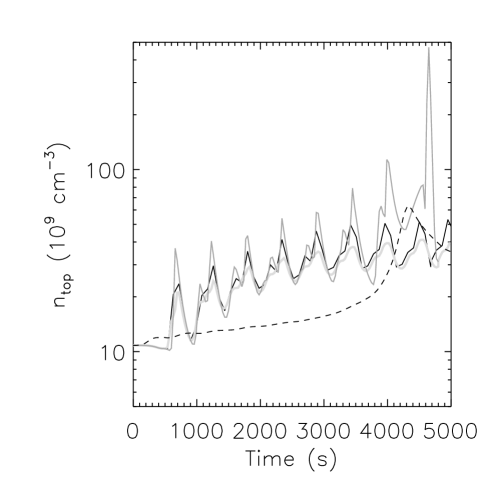
Figure 4.— Evolution of the temperature (left) and the density (right) at the loop top, for different spatial and temporal characteristics of heating: continuous heating concentrated at the foot-point with spatial scale $\sigma=L/3$ (dashed lines), periodic heat pulses with $\sigma=L/3$ (thick light grey), $\sigma=L/5$ (solid black), $\sigma=L/10$ (dark grey).

Figure 4 shows the evolution of the plasma temperature and density at the loop apex for the loop models with pulsed heating as compared with the solution for constant heating. The evolution of the plasma properties at the loop apex are presented for the loop constantly heated at the foot-point ($\sigma=L/3$; dashed lines), and for the loops subject to heat pulses with different spatial distribution: $\sigma=L/3$ (thick light grey); $\sigma=L/5$ (solid black); and $\sigma=L/10$ (dark grey). The figure shows the instability of the constantly heated loop and of the solution with heat too concentrated at the foot-points ($\sigma=L/10$). The two solutions with $\sigma=L/5$ and $\sigma=L/3$ appear more stable.

Effect of Heating Parameters —

The critical parameter for loop stability is the spatial width of the heating function: we have stable solutions for $\sigma\gtrsim L/3$ and unstable solutions for $\sigma\lesssim L/10$; for $\sigma\sim L/5$ the loops are on the edge of stability, and other characteristics of the heating (intensity, interval between pulses) become important. We find consistent results for both the cooler and the hotter solutions.

The interval between pulses, $\tau$, does not appear to be a critical parameter for stability as long as it is not too small ($\tau\ll\tau_{\rm cool}$), i.e. too close to the constant heating case that is unstable for $\sigma=L/3$ (see Fig. 1), nor too long with respect to the cooling time, since the loop would then catastrophically cool.

3.2. Emission Measure Distribution

Besides investigating the stability of the solutions, our modeling effort aims at studying the effect of shrinking the heating region at the loop foot-points on the $EM(T)$, which is one of the main derived quantities that allow us to study and to compare the coronal properties of different stars.

As described in section 2, we analyze two different sets of models with maximum temperatures of about $\sim 3\times 10^{6}$ K, and $\sim 10^{7}$ K, respectively. Since we find results that are qualitatively similar in both cases, we will discuss in detail the model of hotter loop, because one of the questions we want to address is the possibility of reproducing the $EM(T)$ of active stars (generally characterized by peak temperature of the order of $10^{7}$ K) with the proposed model.

From our simulations we can model the global emission of a stellar corona composed of many loops impulsively heated by microflares occurring close to their foot-points. Under the assumption that all of the loops have a statistically analogous evolution, taking a sample of profiles at different times in the evolution of a single loop, as shown for example in Fig. 3, is equivalent to observing all of the loops simultaneously, with each loop at a different stage in its evolution. We take 200 outputs from each simulation, uniformly sampled in time, and consider each output as a snapshot of an independent loop. Thus, the total emission from the corona, composed of all these loops, is the sum of the emission of all the snapshots.

From the temperature and density profiles of each output we derive $EM(T)$ and then we sum them to obtain the global $EM(T)$. We derive $EM(T)$ in each temperature bin, $\Delta T_{i}$, as $EM(T_{i})=\sum_{j}n_{e}^{2}(j)~{}ds_{j}$ where $j$ spans over the spatial bins whose temperature falls within $\Delta T_{i}$, and the temperature bins are constant in $\log T$ such that $\Delta\log T=0.1$. Therefore $EM(T)$ obtained with this procedure differs from the definition of Eq.(1) by a normalization factor that corresponds to the cross-sectional area of the loop.

Figure 5 shows $EM(T)$ for the loop models with average coronal temperatures $\sim 10^{7}$ K, and heating functions with different spatial widths. The solutions with $\sigma=L/3$ (top), $\sigma=L/5$ (middle), and $\sigma=L/10$ (bottom), show the effect on $EM(T)$ of varying the heating concentration. The lines in the lower part of the plots of Figure 5 correspond to $EM(T)$ for each output represented with lines darkening from $t=0$ (light gray) to $t=t_{\rm run}$ (dark gray). The upper thick black line represents the total $EM(T)$, which is the sum of all the individual distributions. Therefore the total $EM(T)$ is the one that would characterize a corona composed entirely of such loops. In order to allow for an easier comparison of the static model with the dynamic simulations, $EM(T)$ of the initial static solution (dashed-dotted line) is also shown arbitrarily shifted next to the total $EM(T)$. In Figure 5 the power laws corresponding to $EM(T)\propto T^{3/2}$ and $EM(T)\propto T^{5}$ are also plotted as useful points of reference, as discussed in §1.

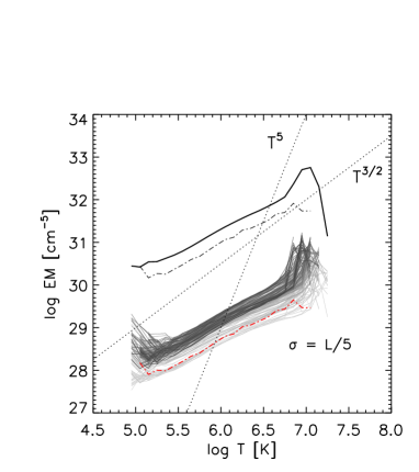
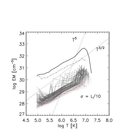
Figure 5.— Emission measure distribution, $EM(T)$, for the solutions with $T_{\rm max}\sim 10^{7}$K, $\langle E_{\rm H}\rangle=4E_{0}$, and $\sigma=L/3$ (top), $\sigma=L/5$ (middle), $\sigma=L/10$ (bottom). The lines in the lower part of the plots correspond to the $EM(T)$ of the individual outputs, regularly sampling the whole loop evolution; the lines get darker from $t=0$ (lighter gray) to $t=t_{\rm run}$ (darker gray lines). The dashed-dotted lines correspond to the $EM(T)$ of the initial static condition, while the upper thick black line is the total $EM(T)$. For comparison the dotted lines indicate the power laws corresponding to $EM(T)\propto T^{3/2}$ and $EM(T)\propto T^{5}$.

The $EM(T)$ of the initial hydrostatic solution is quite flat, close to the $T^{3/2}$ power-law. Figure 5 shows that $EM(T)$ can clearly be used to characterize the dynamic simulations since we see that the total $EM(T)$ changes consistently as the heating becomes more concentrated in the foot-point region. The main difference of the total $EM(T)$ (solid lines) from the standard hydrostatic distribution is the presence of a well-defined peak at high temperatures ($\sim 10^{7}$ K). This is also the temperature range corresponding to the bulk of the emission from active stellar coronae.

For $\sigma=L/3$ the $EM(T)$ is close to the initial curve. Narrowing the region of energy release to $\sigma=L/5$ causes the $EM(T)$ to steepen and approach the scaling derived from stellar observations. The more concentrated the heating, the wider the peak.

The $EM(T)$ does not depend on the parameter $\tau$ as it does on the concentration of the heating.

In Figure 6 we compare the $EM(T)$ derived from our model, for $\sigma=L/5$, to an $EM(T)$ derived by Scelsi et al. (2004) from XMM-Newton spectral observations of the active star 31 Com. The $EM(T)$ derived from a RTV hydrostatic model is also shown. The $EM(T)$ derived from our model, with impulsive foot-point heating, is qualitatively similar to the $EM(T)$ of 31 Com.

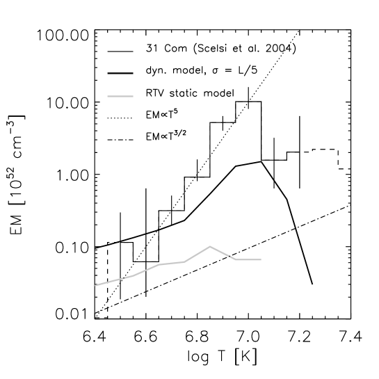
Figure 6.— $EM(T)$ derived for a loop model with maximum temperature $\sim 10^{7}$ K, and foot-point heating ($\sigma=L/5$; thick line), as compared to the $EM(T)$ of 31 Com (histogram) derived from an X-ray spectrum. As a reference, the $EM(T)$ for an RTV hydrostatic model (light grey line), and power-laws with $EM(T)\propto T^{5}$ (dotted line) and $EM(T)\propto T^{3/2}$ (dash-dotted line) are shown as well. $EM(T)$ from models are arbitrarily scaled.

4. Discussion and Conclusions

Coronal loops are known to be unstable if heated continuously in a sufficiently small region at their foot-points. Also, the $EM(T)$ of stable, uniformly-heated loops of constant cross-section is known to obey a power law with index $\sim 3/2$. In the present work, we have investigated the existence of long-lived coronal loops heated by sequences of pulses located at their foot-points and studied the changes induced in the $EM(T)$ by this form of heating. In particular, we examined relatively long ($2\times 10^{10}$ cm) and hot ($\approx 3\times 10^{6}$ K and $10^{7}$ K) loops appropriate to investigating both the solar environment, which we can spatially resolve and compare directly with models, and the coronae of active stars, where evidence of different $EM(T)$ has been found.

We find long-lived dynamically stable solutions in cases with heating concentrated close to the foot-points, with values of $\sigma$ down to $\sim L/5$. Therefore we find stable solutions for much more concentrated heating compared with the solutions of the S81 model; the latter, using a heating spatial distribution of the form $H_{0}e^{-s/s_{\rm H}}$, does not yield stable solutions for $s_{\rm H}\sim L/3$. The value of $\sigma\sim L/5$ represents the border zone between rapidly unstable and long-lived loops for both sets of simulations with different maximum temperatures (see Tab. 1), provided that the heating is strong enough to sustain the loop. We note, however, that close to this boundary some unstable cases appear quasi-steady when observed over time scales that are long compared to the cooling time. We find that the time scales of the loops’ evolution do not critically depend on the intensity of the heating, or on the period of heat pulses, with the caveats discussed in the previous section.

Our work has therefore proven that long-lived footpoint-heated loops can exist, provided that the heating is intermittent with the appropriate period – a fraction of the loop cooling time – which should be long enough to depart from continuous heating, but shorter than the loop plasma cooling time. The intermittent heating allows the plasma at the loop apex to drain downward to the chromospheric region (as confirmed by the downward velocity of the plasma close to the apex in between the pulses), and prevents the accumulation of the plasma at the loop top, and thus the thermal instability. Our results are in agreement with those of other works modeling footpoint-heated loops (e.g., Müller et al., 2004).

In the present work we also showed that the $EM(T)$ of foot-point heated loops are significantly different to those of conventional hydrostatic loops. The $EM(T)$ of foot-point heated loops shows a well-defined peak, which becomes wider and wider as the heating becomes more concentrated towards the foot-points. This holds true for both sets of simulations at different temperatures analyzed here (see Tab. 1). The low temperature side of the peaks has a steeper slope than the $EM(T)\propto T^{3/2}$ of the static case. The slope found for the stable cases with smaller $\sigma$ approaches the power law of $EM(T)\propto T^{5}$. We note, in passing, that loops with coronal cross-section larger than in their chromospheres may give similar results (e.g., Schrijver et al., 1989; Ciaravella et al., 1996; Sim & Jordan, 2003). We plan to investigate this possibility in the future.

The $EM(T)$ of the impulsively heated loops modeled here show a qualitative agreement with those derived from several X-ray and EUV spectroscopic observations of active stars. Recent analyses outline a scenario in which hotter ($T\sim 10^{7}$ K) plasma is characterized by physical conditions that are fundamentally different from the cooler ($T\lesssim 3\times 10^{6}$ K) plasma, which probably belongs to a different class of structures. In particular, there is increasing observational evidence of hot plasma with density two orders of magnitude higher than the cooler plasma. These density and filling factor results (e.g., Testa et al., 2004) support a scenario in which, for increasing activity levels, significant flaring activity may be present, yielding the hotter plasma structures. In such a scenario, it is likely that hot loops are sustained by impulsive energy release. Therefore, the theoretical model discussed here is based on assumptions that are consistent with the observational evidence, while reproducing the steep and peaked $EM(T)$ widely found for active stars.

There is room for several improvements to be made to our model: we plan to model loops with a larger cross-section in the corona; and we will consider the larger set of models for unstable, foot-point heated loops, since the superposition of several loops of this kind may help to explain unresolved, monolithic loop structures composed of many strands, or even whole stellar coronae.

References

- Antiochos (1979) Antiochos, S. K. 1979, ApJ, 232, L125
- Argiroffi et al. (2003) Argiroffi, C., Maggio, A., & Peres, G. 2003, A&A, 404, 1033
- Aschwanden (2001) Aschwanden, M. J. 2001, ApJ, 559, L171
- Aschwanden et al. (2000) Aschwanden, M. J., Nightingale, R. W., & Alexander, D. 2000, ApJ, 541, 1059
- Aschwanden et al. (2001) Aschwanden, M. J., Schrijver, C. J., & Alexander, D. 2001, ApJ, 550, 1036
- Betta et al. (1997) Betta, R., Peres, G., Reale, R., & Serio, S. 1997, A&AS, 122, 585
- Brekke et al. (1997) Brekke, P., Kjeldseth-Moe, O., Brynildsen, N., et al. 1997, Sol. Phys., 170, 163
- Brosius et al. (1996) Brosius, J. W., Davila, J. M., Thomas, R. J., & Monsignori-Fossi, B. C. 1996, ApJS, 106, 143
- Cargill (1994) Cargill, P. J. 1994, ApJ, 422, 381
- Cargill & Klimchuk (1997) Cargill, P. J. & Klimchuk, J. A. 1997, ApJ, 478, 799
- Cargill & Klimchuk (2004) —. 2004, ApJ, 605, 911
- Ciaravella et al. (1996) Ciaravella, A., Peres, G., Maggio, A., & Serio, S. 1996, A&A, 306, 553
- Drake (1996) Drake, J. J. 1996, in ASP Conf. Ser. 109: Cool Stars, Stellar Systems, and the Sun, 203–+
- Drake et al. (2000) Drake, J. J., Peres, G., Orlando, S., Laming, J. M., & Maggio, A. 2000, ApJ, 545, 1074
- Dupree (1996) Dupree, A. K. 1996, in ASP Conf. Ser. 109: Cool Stars, Stellar Systems, and the Sun, 237–+
- Dupree (2002) Dupree, A. K. 2002, in ASP Conf. Ser. 277: Stellar Coronae in the Chandra and XMM-NEWTON Era, 201–+
- Dupree et al. (1993) Dupree, A. K., Brickhouse, N. S., Doschek, G. A., Green, J. C., & Raymond, J. C. 1993, ApJ, 418, L41+
- Giampapa et al. (1985) Giampapa, M. S., Golub, L., Peres, G., Serio, S., & Vaiana, G. S. 1985, ApJ, 289, 203
- Golub (2004) Golub, L. 2004, in COSPAR, Plenary Meeting
- Griffiths & Jordan (1998) Griffiths, N. W. & Jordan, C. 1998, ApJ, 497, 883
- Jordan (1980) Jordan, C. 1980, A&A, 86, 355
- Klimchuk & Cargill (2001) Klimchuk, J. A. & Cargill, P. J. 2001, ApJ, 553, 440
- Landi & Landini (1997) Landi, E. & Landini, M. 1997, A&A, 327, 1230
- Landini et al. (1985) Landini, M., Monsignori-Fossi, B. C., & Pallavicini, R. 1985, Space Science Reviews, 40, 43
- Müller et al. (2004) Müller, D. A. N., Peter, H., & Hansteen, V. H. 2004, A&A, 424, 289
- Mewe et al. (2001) Mewe, R., Raassen, A. J. J., Drake, J. J., et al. 2001, A&A, 368, 888
- Orlando et al. (2000) Orlando, S., Peres, G., & Reale, F. 2000, ApJ, 528, 524
- Pallavicini et al. (1981) Pallavicini, R., Peres, G., Serio, S., et al. 1981, ApJ, 247, 692
- Peres et al. (2001) Peres, G., Orlando, S., Reale, F., & Rosner, R. 2001, ApJ, 563, 1045
- Peres et al. (2000) Peres, G., Orlando, S., Reale, F., Rosner, R., & Hudson, H. 2000, ApJ, 528, 537
- Peres et al. (1993) Peres, G., Reale, F., & Serio, S. 1993, in ASSL Vol. 183: Physics of Solar and Stellar Coronae, 151
- Peres et al. (1987) Peres, G., Reale, F., Serio, S., & Pallavicini, R. 1987, ApJ, 312, 895
- Peres et al. (1982) Peres, G., Serio, S., Vaiana, G. S., & Rosner, R. 1982, ApJ, 252, 791
- Priest et al. (2000) Priest, E. R., Foley, C. R., Heyvaerts, J., et al. 2000, ApJ, 539, 1002
- Reale (2002) Reale, F. 2002, ApJ, 580, 566
- Reale et al. (1988) Reale, F., Peres, G., Serio, S., Rosner, R., & Schmitt, J. H. M. M. 1988, ApJ, 328, 256
- Rosner et al. (1978) Rosner, R., Tucker, W. H., & Vaiana, G. S. 1978, ApJ, 220, 643
- Rosner & Vaiana (1977) Rosner, R. & Vaiana, G. S. 1977, ApJ, 216, 141
- Sanz-Forcada et al. (2002) Sanz-Forcada, J., Brickhouse, N. S., & Dupree, A. K. 2002, ApJ, 570, 799
- Sanz-Forcada et al. (2003) —. 2003, ApJS, 145, 147
- Scelsi et al. (2004) Scelsi, L., Maggio, A., Peres, G., & Gondoin, P. 2004, A&A, 413, 643
- Schrijver et al. (1989) Schrijver, C. J., Lemen, J. R., & Mewe, R. 1989, ApJ, 341, 484
- Serio et al. (1981) Serio, S., Peres, G., Vaiana, G. S., Golub, L., & Rosner, R. 1981, ApJ, 243, 288
- Serio et al. (1991) Serio, S., Reale, F., Jakimiec, J., Sylwester, B., & Sylwester, J. 1991, A&A, 241, 197
- Sim & Jordan (2003) Sim, S. A. & Jordan, C. 2003, MNRAS, 346, 846
- Spadaro et al. (2003) Spadaro, D., Lanza, A. F., Lanzafame, A. C., et al. 2003, ApJ, 582, 486
- Spitzer (1962) Spitzer, L. 1962, Physics of Fully Ionized Gases (Physics of Fully Ionized Gases, New York: Interscience (2nd edition), 1962)
- Testa et al. (2004) Testa, P., Drake, J., & Peres, G. 2004, ApJ, 617, 508
- Testa & Peres (2003) Testa, P. & Peres, G. 2003, AAS/Solar Physics Division Meeting, 34, 17.02
- Testa et al. (2002) Testa, P., Peres, G., Reale, F., & Orlando, S. 2002, ApJ, 580, 1159
- Vaiana et al. (1973) Vaiana, G. S., Krieger, A. S., & Timothy, A. F. 1973, Sol. Phys., 32, 81
- Vernazza et al. (1976) Vernazza, J. E., Avrett, E. H., & Loeser, R. 1976, ApJS, 30, 1
- Vesecky et al. (1979) Vesecky, J. F., Antiochos, S. K., & Underwood, J. H. 1979, ApJ, 233, 987
- Warren et al. (2002) Warren, H. P., Winebarger, A. R., & Hamilton, P. S. 2002, ApJ, 579, L41
- Warren et al. (2003) Warren, H. P., Winebarger, A. R., & Mariska, J. T. 2003, ApJ, 593, 1174
- Winebarger et al. (2002) Winebarger, A. R., Warren, H., van Ballegooijen, A., DeLuca, E. E., & Golub, L. 2002, ApJ, 567, L89
- Winebarger et al. (2003) Winebarger, A. R., Warren, H. P., & Mariska, J. T. 2003, ApJ, 587, 439