Semi-empirical analysis of SDSS galaxies: I. Spectral synthesis method

Abstract

The study of stellar populations in galaxies is entering a new era with the availability of large and high quality databases of both observed galactic spectra and state-of-the-art evolutionary synthesis models. In this paper we investigate the power of spectral synthesis as a mean to estimate physical properties of galaxies. Spectral synthesis is nothing more than the decomposition of an observed spectrum in terms of a superposition of a base of simple stellar populations of various ages and metallicities, producing as output the star-formation and chemical histories of a galaxy, its extinction and velocity dispersion. Our implementation of this method uses the Bruzual & Charlot (2003) models and observed spectra in the 3650–8000 Å range. The reliability of this approach is studied by three different means: (1) simulations, (2) comparison with previous work based on a different technique, and (3) analysis of the consistency of results obtained for a sample of galaxies from the Sloan Digital Sky Survey (SDSS).

We find that spectral synthesis provides reliable physical parameters as long as one does not attempt a very detailed description of the star-formation and chemical histories. Robust and physically interesting parameters are obtained by combining the (individually uncertain) strengths of each simple stellar population in the base. In particular, we show that besides providing excellent fits to observed galaxy spectra, this method is able to recover useful information on the distributions of stellar ages and, more importantly, stellar metallicities. Stellar masses, velocity dispersion and extinction are also found to be accurately retrieved for realistic signal-to-noise ratios.

We apply this synthesis method to a volume limited sample of 50362 galaxies from the SDSS Data Release 2, producing a catalog of stellar population properties. Emission lines are also studied, their measurement being performed after subtracting the computed starlight spectrum from the observed one. A comparison with recent estimates of both observed and physical properties of these galaxies obtained by other groups shows good qualitative and quantitative agreement, despite substantial differences in the method of analysis. The confidence in the method is further strengthened by several empirical and astrophysically reasonable correlations between synthesis results and independent quantities. For instance, we report the existence of strong correlations between stellar and nebular metallicites, stellar and nebular extinctions, mean stellar age and equivalent width of H$\alpha$ and 4000 Å break, and between stellar mass and velocity dispersion.

1 Introduction

Galaxy spectra encode information on the age and metallicity distributions of the constituent stars, which in turn reflect the star-formation and chemical histories of the galaxies. Retrieving this information from observational data in a reliable way is crucial for a deeper understanding of galaxy formation and evolution.

The mapping of observed onto physical properties of galaxies has been a major topic of research for over a generation of astronomers since the pioneering works of Morgan (1956), Wood (1966) and Faber (1972) on the one hand, and Tinsley (1968) and Spinrad & Taylor (1972) on the other. The first group of authors introduced the so-called empirical population synthesis methods, which aim at reproducing a set of observations of a given galaxy by means of a linear combination of simpler systems of known characteristics, like individual stars or chemically homogeneous and coeval groups of stars. Bica (1988), Pelat (1997), Cid Fernandes et al. (2001), Moultaka et al. (2004) are examples of modern studies following this approach. The second group pioneered the so-called evolutionary population synthesis methods, which compare galaxy data with models that follow the time evolution of an entire stellar system by combining libraries of evolutionary tracks and stellar spectra with prescriptions for the initial mass function (IMF), star formation and chemical histories. This approach has enjoyed more widespread use in recent years, e.g., Arimoto & Yoshii (1987), Guiderdoni & Rocca-Volmerange (1987), Bressan et al. (1994), Fioc & Rocca-Volmerange (1997), Vazdekis (1999), Bruzual & Charlot (2003, hereafter BC03), Le Borgne et al. (2004), among many others (see Cardiel et al. 2003 for a large set of references). In short, empirical synthesis relies on nature for its basic ingredients, whereas evolutionary synthesis relies mostly on models. However, since models are made and calibrated to mimic nature, this difference is gradually vanishing as models improve.

Besides different methodologies, there are also differences in what type of data is actually modeled. Colours (e.g., Wood 1966), absorption line equivalent widths or spectral indices (e.g., Worthey 1994; Kauffmann et al. 2003, hereafter K03) and emission features, both stellar (Leitherer, Robert & Heckman 1995; Schaerer & Vacca 1998) and nebular (Mas-Hesse & Kunth 1991; Kewley et al. 2001), have all been used in stellar population synthesis. More recently, the full spectral information has been incorporated in the modeling process, both including (Charlot & Longhetti 2001), and excluding emission lines (Vazdekis & Arimoto 1999; Reichardt, Jimenez & Heavens 2001; Cid Fernandes et al. 2004a, hereafter CF04).

Recovering the stellar content of a galaxy from its observed integrated spectrum is not an easy task, as can be deduced from the amount of work devoted to this topic over the past $\sim$ half century. The situation is however much more favorable nowadays. Huge observational and theoretical efforts in the past few years have produced large sets of high quality spectra of stars (e.g., Prugniel & Soubiran 2001; Le Borgne et al. 2003; Bertone et al. 2004; González Delgado et al. 2004). These libraries are being implemented in a new generation of evolutionary synthesis models, allowing the prediction of galaxy spectra with an unprecedented level of detail (Vazdekis 1999; BC03, Le Borgne et al. 2004). At the same time, galaxy spectra are now more abundant than ever (Loveday et al. 1996; York et al. 2000). The Sloan Digital Sky Survey (SDSS), in particular, is providing a homogeneous data base of hundreds of thousands of galaxy spectra in the 3800–9200 Å range, with a resolution of $\lambda/\Delta\lambda\sim 1800$ (York et al. 2000; Stoughton et al. 2002; Abazajian et al. 2003, 2004). This enormous amount of high quality data will undoubtedly be at the heart of tremendous progress in our understanding of galaxy constitution, formation and evolution. Indeed, significant steps in this direction have recently been made (K03; Brinchmann et al. 2004, Tremonti et al. 2004; Heavens et al. 2004; Panter, Heavens & Jimenez 2004).

In order to take advantage of the recent progress in evolutionary synthesis to analyze data sets such as the SDSS, a methodology must be set up to go from the observed spectra to physical properties of galaxies. In this paper we discuss one possible method to achieve this goal. The method is based on fitting an observed spectrum with a linear combination of simple theoretical stellar populations (coeval and chemically homogeneous) computed with evolutionary synthesis models at the same spectral resolution as that of the SDSS.

Our goal here is to demonstrate that, besides providing excellent starlight templates to aid emission line studies, spectral synthesis recovers reliable stellar population properties out of galaxy spectra of realistic quality. We show that this simple method provides robust information on the stellar age ($t_{\star}$) and stellar metallicities ($Z_{\star}$) distributions, as well as on the extinction, velocity dispersion and stellar mass. The ability to recover information on $Z_{\star}$ is particularly welcome, given that stellar metallicities are notoriously more difficult to assess than other properties. In order to reach this goal we follow: (1) a priori arguments, based on simulations; (2) comparisons with independent work based on a different method, and (3) an a posteriori empirical analysis of the consistency of results obtained for a large sample of SDSS galaxies. Other papers in this series on the Semi-Empirical Analysis of Galaxies (SEAGal) will explore various astrophysical implications of the results obtained with this method.

This paper is organized as follows. Section 2 presents an overview of our synthesis method and simulations designed to test it and evaluate the uncertainties involved. The discussion is focused on how to use the synthesis to derive robust estimators of physically interesting stellar population properties. Section 3 defines a volume limited sample of SDSS galaxies and presents the results of the synthesis of their spectra, along with measurements of emission lines. In Section 4 we compare our results to those recently published by Brinchmann et al. (2004). Stellar population and emission line properties are used in Section 5 to investigate whether the synthesis produces astrophysically plausible results. Finally, Section 6 summarizes our main findings.

2 Spectral Synthesis

2.1 Method

Our synthesis code, which we call STARLIGHT, was first discussed in CF04 (see also Cid Fernandes et al. 2004b and Garcia-Rissman et al. 2005 for different applications of the same code). STARLIGHT mixes computational techniques originally developed for empirical population synthesis with ingredients from evolutionary synthesis models. Briefly, we fit an observed spectrum $O_{\lambda}$ with a combination of $N_{\star}$ Simple Stellar Populations (SSP) from the evolutionary synthesis models of BC03. Extinction is modeled as due to foreground dust, and parametrized by the V-band extinction $A_{V}$. The Galactic extinction law of Cardelli, Clayton & Mathis (1989) with $R_{V}=3.1$ is adopted. Line of sight stellar motions are modeled by a Gaussian distribution $G$ centered at velocity $v_{\star}$ and with dispersion $\sigma_{\star}$. With these assumptions the model spectrum is given by

$$M_{\lambda}=M_{\lambda_{0}}\left[\sum_{j=1}^{N_{\star}}x_{j}b_{j,\lambda}r_{\lambda}\right]\otimes G(v_{\star},\sigma_{\star})$$ (1)

where $b_{j,\lambda}$ is the spectrum of the $j^{\rm th}$ SSP normalized at $\lambda_{0}$, $r_{\lambda}\equiv 10^{-0.4(A_{\lambda}-A_{\lambda_{0}})}$ is the reddening term, $M_{\lambda_{0}}$ is the synthetic flux at the normalization wavelength, $\vec{x}$ is the population vector and $\otimes$ denotes the convolution operator. Each component $x_{j}$ ($j=1\ldots N_{\star}$) represents the fractional contribution of the SSP with age $t_{j}$ and metallicity $Z_{j}$ to the model flux at $\lambda_{0}$. The base components can be equivalently expressed as a mass fractions vector $\vec{\mu}$. In this work we adopt a base with $N_{\star}=45$ SSPs, encompassing 15 ages between $10^{6}$ and $1.3\times 10^{10}$ yr and 3 metallicities: $Z=0.2$, 1 and 2.5 $Z_{\odot}$. Their spectra, shown in Fig. 1, were computed with the STELIB library (Le Borgne et al. 2003), Padova 1994 tracks, and Chabrier (2003) IMF (see BC03 for details).

The fit is carried out with a simulated annealing plus Metropolis scheme which searches for the minimum $\chi^{2}=\sum_{\lambda}\left[\left(O_{\lambda}-M_{\lambda}\right)w_{\lambda}\right]^{2}$, where $w_{\lambda}^{-1}$ is the error in $O_{\lambda}$. Regions around emission lines, bad pixels or sky residuals are masked out by setting $w_{\lambda}=0$. Pixels which deviate by more than 3 times the rms between $O_{\lambda}$ and an initial estimate of $M_{\lambda}$ are also given zero weight.

The minimization consists of a series of $N_{M}=6$ likelihood-guided Metropolis explorations of the parameter space. From each iteration to the next we increase the $w_{\lambda}$ weights geometrically (which corresponds to a decrease in the “temperature” in statistical mechanics terms; e.g., MacKay 2003). The step-size in each parameter is concomitantly decreased and the number of steps is increased. This scheme gradually focuses on the most likely region in parameter space, avoiding (through the logic of the Metropolis algorithm) trapping onto local minima. After completion, the whole fit is fine tuned repeating the full loop excluding all $x_{j}=0$ components. An important difference (from the computational point of view) with respect to the code in CF04 is that we now perform a series expansion of the $r_{\lambda}$ extinction factor, which allows a much faster computation of $\chi^{2}$. Naturally, there are a number of technical parameters in this complex fitting algorithm, which we have optimized by means of extensive simulations (see CF04). At any rate, results reported here are robust with respect to variations in these technical parameters.

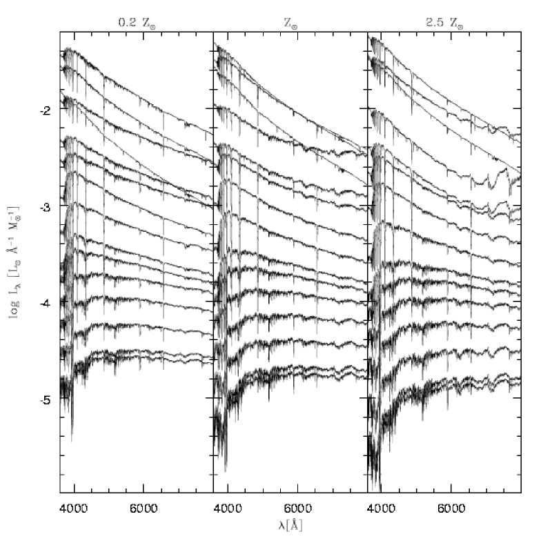
Figure 1: Spectra of the 45 SSPs used in the spectral synthesis (from BC03). The base comprises 3 different metallicities, $Z=0.2$, 1 and 2.5 $Z_{\odot}$, and 15 ages: From top to bottom, $t=$ 0.001, 0.00316, 0.00501, 0.01, 0.02512, 0.04, 0.10152, 0.28612, 0.64054, 0.90479, 1.434, 2.5, 5, 11 and 13 Gyr. All SSPs are normalized to 1 M_⊙ at $t=0$.

Figs. 2 and 3 illustrate the spectral fits obtained for two galaxies drawn from the SDSS database. The top-left panel shows the observed spectrum (thin line) and the model (thick), as well as the error spectrum (dashed). The bottom-left panel shows the $O_{\lambda}-M_{\lambda}$ residual spectrum, while the panels in the right summarize the derived star-formation history encoded in the age-binned population vector. These examples, along with those in K03 and CF04, demonstrate that this simple method is capable of reproducing real galaxy spectra to an excellent degree of accuracy.

An important application of the synthesis is to measure emission lines from the residual spectrum, as done by K03 (see also Section 3.3). Another, of course, is to infer stellar population properties from the fit parameters. This was not the approach followed by K03 and their subsequent papers, who prefer to derive stellar population properties mainly from the $D_{n}(4000)$ versus H$\delta_{A}$ diagram. Our central goal here is to investigate whether spectral synthesis can also recover reliable stellar population properties. In the remainder of this section we address this issue by means of simulations.

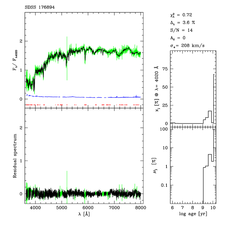
Figure 2: Spectral synthesis of an early type SDSS galaxy. Top-left: Observed (thin, green line), model (thick, black ) and error spectra (dashed, blue). Points in the bottom indicate bad pixels (as given by the SDSS flag) or emission lines windows, both of which were masked out in the fits. Bottom-left: Residual spectrum. Masked regions are plotted with a thin, green line. Right: Flux (top) and mass (bottom) fractions as a function of age. Some of the derived properties are listed in the top-right. $\chi^{2}_{\lambda}$ is the reduced $\chi^{2}$, and $\Delta_{\lambda}$ is the mean relative difference between model and observed spectra; $S/N$ refers to the region around $\lambda_{0}=4020$ Å.

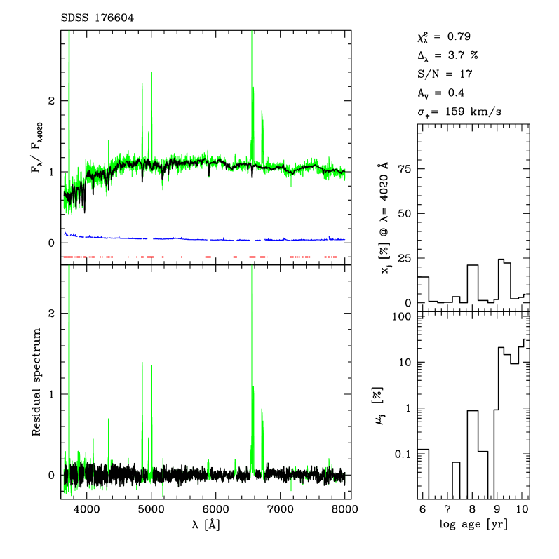
Figure 3: As Fig. 2 but for a late-type galaxy.

2.2 Robust description of the synthesis results

The existence of multiple solutions is an old known problem in stellar population synthesis. This multiplicity arises from a combination of three factors: (1) algebraic degeneracy (number of unknowns larger than number of observables), (2) intrinsic degeneracies of stellar populations and (3) measurement uncertainties. Unlike in methods which synthesize only a handful of spectral indices, algebraic degeneracy is not a problem for the method outlined above, as the number of $O_{\lambda}$ points in any decently sampled spectrum far exceeds the number of parameters even for large bases. Similarly, by modeling the whole spectrum one should be able to alleviate degeneracies in spectral indices associated with different stellar populations (Jimenez et al. 2004). Measurement errors, however, are still a problem. A corollary of these complications is that even superb spectral fits as those shown in Figs. 2 and 3 do not guarantee that the resulting parameter estimates are trustworthy.

This brief discussion illustrates the need to assess the degree to which one can trust the parameters involved in the fit before using them to infer stellar populations properties. As posed above, the spectral fits involve $N_{\star}+3$ parameters: $N_{\star}-1$ of the $\vec{x}$ components (one degree of freedom is removed by the normalization constraint), $M_{\lambda_{0}}$, $A_{V}$ and the two kinematical parameters, $v_{\star}$ and $\sigma_{\star}$. The reliability of parameter estimation is best studied by means of simulations which feed the code with spectra generated with known parameters, add noise, and then examine the correspondence between input and output values.

CF04 performed this kind of simulation for a $N_{\star}=20$ base and spectra in the 3500–5200 Å interval. Their analysis concentrated on how well the method recovers $\vec{x}_{\rm input}$ for varying degrees of noise. The main results of that study are: (1) In the absence of noise, the method recovers all components of $\vec{x}$ to a high degree of accuracy. (2) In the presence of noise, however, the individual output $x_{j}$ fractions may deviate drastically from the input values. Essentially, what happens is that noise washes away the differences between spectrally similar components, so it becomes impossible to distinguish them, and the code splits $x_{j}$ among neighboring components in spectral space. This is a common problem in population synthesis (e.g., Panter et al. 2004; Tremonti 2003; Cid Fernandes et al. 2001).

Once we have identified the origin of the problem, the remedy to fix it is evident: bin-over spectrally similar components. In other words, instead of attempting a fine graded description of stellar populations mixtures in terms of many ages and metallicities, it is much better to “marginalize over the details” and work with a coarser but more robust description based on combined $x_{j}$ fractions. As shown by CF04, condensed versions of the population vector which project its $N_{\star}$ components onto just a few physically interesting axes, yield very reliable results.

Our approach and objectives are conceptually similar to those of the MOPED code of Heavens, Jimenez & Lahav (2000; see also Reichardt et al. 2001, Panter et al. 2004). Operationally, however, the two codes differ. MOPED compresses data on input by degrading the SDSS spectral resolution to 20 Å and performing weighted linear combinations of $O_{\lambda}$, reducing its dimension to one datum per output parameter while at the same time minimizing the loss of information. STARLIGHT, on the other hand, works with the spectrum at its full resolution and an overdimensioned set of parameters (i.e., large $N_{\star}$), which we compress on the description of the output. The disadvantage of our approach is computational. Indeed, it is described as a “slow” and “brute force” method by Panter et al. (2004). This, however, is not a severe problem given the abundance of CPUs nowadays (STARLIGHT takes about 4 minutes per galaxy on a 2 GHz Linux-workstation). Furthermore, there is plenty of room for improvement in the efficiency of the algorithm, for instance, by implementing a smarter exploration of the parameter space (Slosar & Hobson 2003), to the point that computational constraints could soon become a minor concern. An advantage of STARLIGHT is that it also measures kinematical parameters (mainly $\sigma_{\star}$) and provides a high resolution template spectrum.

2.2.1 Simulations

We have carried out new simulations designed to test the method and investigate which combinations of the parameters provide robust results. These simulations differ from those in CF04 in three main aspects: (1) the spectral range is now 3650–8000 Å; (2) the new base is larger; (3) a more realistic error spectrum was used. A further difference is that we use a larger number of iterations, partly because we have more base elements than CF04 and partly because the code is now over 200 times faster. At each step in the annealing scheme, the number of steps per parameter is set to $2L/\epsilon$, where $L$ is the length of the allowed range for the parameter (e.g., $L=1$ for $x_{j}$ fractions, which range from 0 to 1), and $\epsilon$ is the step-size (see CF04 for a more detailed description of these technical aspects). This insures that each parameter can in principle random-walk twice its whole allowed range, which is an adequate criterion for Metropolis sampling (e.g., MacKay 2003). Furthermore, there are 12 stages in the annealing schedule. Overall, over $10^{7}$ combinations of parameters are sampled for each galaxy.

Several sets of simulations were performed. Given our interest in modeling SDSS galaxies, here we focus on simulations tailored to match the characteristics of this data set. Test galaxies were built from the average $\vec{x}$, $A_{V}$ and $\sigma_{\star}$ within 65 boxes in the mean stellar age versus mean stellar metallicity plane obtained for the sample described in Section 3. Each spectrum covers the 3650–8000 Å range in steps of 1 Å, the same sampling of the BC03 models. We generate 20 perturbed versions of each synthetic spectrum for each of 5 levels of noise: $S/N=5$, 10, 15, 20 and 30, where $S/N$ is the signal-to-noise ratio per Å in the region around $\lambda_{0}=4020$ Å. Unlike in CF04, who used a flat error spectrum, the error at each $\lambda$ was assumed to follow a Gaussian distribution with amplitude obtained by scaling a normalized mean SDSS error spectrum to yield the desired $S/N$ at $\lambda_{0}$. This error spectrum decreases by a factor of $\sim 3$ from 3650 to 6200 Å and then increases again by $\sim 1.5$ towards 8000 Å. Finally, as for the actual data fits, we mask points around [O ii]$\lambda\lambda$3726,3729, [Ne iii]$\lambda 3869$, H$\epsilon$, H$\delta$, H$\gamma$, H$\beta$, [O iii]$\lambda\lambda$4959,5007, [He i]$\lambda 5876$, NaD$\lambda 5890$, [O i]$\lambda$6300, [N ii]$\lambda$$\lambda$6548,6583, H$\alpha$, [S ii]$\lambda\lambda$6717,6731.

These new simulations confirm that the individual components of $\vec{x}$ are very uncertain, so we skip a detailed comparison between $\vec{x}_{\rm input}$ and $\vec{x}_{\rm output}$ and jump straight to results based on more robust descriptions of the synthesis output.

2.2.2 Condensed population vector

Figure 4: Input versus output synthesis parameters for simulations with $S/N=15$ at $\lambda_{0}=4020$ Å. The units are percentages for the condensed population vector ($x_{Y},x_{I},x_{O}$), magnitudes for $A_{V}$, km s^-1 for $\sigma_{\star}$ and arbitrary for $M_{\star}$. The output parameters are represented by $\pm 1$ sigma error bars centered on the mean values obtained by fitting 20 realizations of each of 65 test galaxies.

A coarse but robust description of the star-formation history of a galaxy may be obtained by binning $\vec{x}$ onto “Young” ($t_{j}<10^{8}$ yr), “Intermediate-age” ($10^{8}\leq t_{j}\leq 10^{9}$ yr), and “Old” ($t_{j}>10^{9}$ yr) components ($x_{Y}$, $x_{I}$ and $x_{O}$ respectively). These age-ranges were defined on the basis of the simulations, by seeking which combinations of $x_{j}$’s produce smaller input $-$ output residuals. Table 1 and figure 4 show that these 3 components are very well recovered by the method, with uncertainties smaller than $\Delta x_{Y}=0.05$, $\Delta x_{I}=0.1$, and $\Delta x_{O}=0.1$ for $S/N\geq 10$.

Summary of parameter uncertainties
Parameter	$S/N$ at $\lambda=4020$ Å
	5	10	15	20	30
$x_{Y}$	0.35 $\pm$ 7.06	0.21 $\pm$ 4.50	0.62 $\pm$ 4.04	0.56 $\pm$ 3.04	0.64 $\pm$ 2.63
$x_{I}$	0.76 $\pm$ 13.94	-0.06 $\pm$ 9.00	0.01 $\pm$ 7.88	-0.22 $\pm$ 6.26	-0.02 $\pm$ 5.07
$x_{O}$	-1.12 $\pm$ 13.02	-0.15 $\pm$ 8.83	-0.63 $\pm$ 7.61	-0.34 $\pm$ 6.19	-0.62 $\pm$ 5.05
$\mu_{Y}$	0.02 $\pm$ 1.66	0.11 $\pm$ 1.41	0.16 $\pm$ 1.18	0.18 $\pm$ 1.05	0.19 $\pm$ 0.80
$\mu_{I}$	1.11 $\pm$ 10.26	0.99 $\pm$ 7.57	0.93 $\pm$ 6.10	1.00 $\pm$ 5.03	1.17 $\pm$ 4.22
$\mu_{O}$	-1.13 $\pm$ 10.54	-1.10 $\pm$ 8.17	-1.09 $\pm$ 6.54	-1.18 $\pm$ 5.59	-1.36 $\pm$ 4.63
$A_{V}$	0.01 $\pm$ 0.09	0.00 $\pm$ 0.05	0.01 $\pm$ 0.03	0.01 $\pm$ 0.03	0.00 $\pm$ 0.02
$v_{\star}$	0.24 $\pm$ 17.73	-0.11 $\pm$ 8.55	0.07 $\pm$ 5.92	0.00 $\pm$ 4.23	0.05 $\pm$ 2.81
$\sigma_{\star}$	-3.12 $\pm$ 24.32	-1.40 $\pm$ 12.36	-1.01 $\pm$ 7.71	-0.75 $\pm$ 5.73	-0.57 $\pm$ 3.78
$\log M_{\star}$	0.01 $\pm$ 0.11	-0.01 $\pm$ 0.08	-0.01 $\pm$ 0.06	-0.01 $\pm$ 0.05	-0.02 $\pm$ 0.04
$<\log t_{\star}>_{L}$	-0.01 $\pm$ 0.14	0.01 $\pm$ 0.08	0.00 $\pm$ 0.06	0.01 $\pm$ 0.05	0.01 $\pm$ 0.04
$<\log t_{\star}>_{M}$	-0.03 $\pm$ 0.20	-0.04 $\pm$ 0.14	-0.03 $\pm$ 0.11	-0.04 $\pm$ 0.10	-0.04 $\pm$ 0.08
$\log<Z_{\star}>_{L}$	-0.01 $\pm$ 0.15	-0.01 $\pm$ 0.09	0.00 $\pm$ 0.08	0.00 $\pm$ 0.06	0.00 $\pm$ 0.05
$\log<Z_{\star}>_{M}$	-0.03 $\pm$ 0.18	-0.02 $\pm$ 0.13	-0.03 $\pm$ 0.11	-0.02 $\pm$ 0.09	-0.03 $\pm$ 0.08
$\sigma_{L}(\log t_{\star})$	0.03 $\pm$ 0.16	0.00 $\pm$ 0.10	0.00 $\pm$ 0.08	-0.01 $\pm$ 0.07	-0.01 $\pm$ 0.06
$\sigma_{M}(\log t_{\star})$	-0.04 $\pm$ 0.09	-0.02 $\pm$ 0.06	-0.01 $\pm$ 0.05	-0.01 $\pm$ 0.04	0.00 $\pm$ 0.04
$\sigma_{L}(Z_{\star})$	-0.01 $\pm$ 0.21	0.00 $\pm$ 0.14	0.02 $\pm$ 0.11	0.02 $\pm$ 0.10	0.02 $\pm$ 0.09
$\sigma_{M}(Z_{\star})$	-0.11 $\pm$ 0.26	-0.05 $\pm$ 0.19	-0.03 $\pm$ 0.16	-0.02 $\pm$ 0.14	-0.02 $\pm$ 0.12
$\chi^{2}/N_{\lambda}$	0.95 $\pm$ 0.02	0.95 $\pm$ 0.02	0.95 $\pm$ 0.02	0.95 $\pm$ 0.02	0.95 $\pm$ 0.02
$\Delta_{\lambda}$	11.64 $\pm$ 4.05	5.37 $\pm$ 1.19	3.54 $\pm$ 0.78	2.65 $\pm$ 0.58	1.76 $\pm$ 0.39
$\Delta_{\lambda}\times(S/N)_{\lambda_{0}}$	0.78 $\pm$ 0.27	0.68 $\pm$ 0.20	0.64 $\pm$ 0.21	0.59 $\pm$ 0.22	0.51 $\pm$ 0.23

Table 1: Each line corresponds to a parameter constructed by combining the parameters given by the synthesis. The different columns list the mean $\pm$ rms difference between output and input values of the corresponding quantity, as obtained from simulations with different signal-to-noise ratios. For instance, the mean output minus input difference in $<\log t_{\star}>_{L}$ for $S/N=10$ is 0.01 dex and the rms dispersion is 0.08 dex. The last 3 lines describe the statistics of goodness-of-fit indicators. The units are percentage for light and mass fractions ($x_{Y}\ldots\mu_{O}$), mag for $A_{V}$, km s^-1 for $v_{\star}$ and $\sigma_{\star}$, percentage for $\Delta_{\lambda}$ and dex for logarithmic quantities.

2.2.3 Mass, extinction and velocity dispersion

Fig. 4 also shows the input versus output values of $A_{V}$, $\sigma_{\star}$ and the stellar mass $M_{\star}$. The latter is not an explicit input parameter of the models, but may be computed from $\vec{\mu}$ and the $M_{\star}/L_{\lambda_{0}}$ ratio of the different populations in the base. The uncertainties in these parameters are $\Delta A_{V}<0.05$ mag, $\Delta\log M_{\star}<0.1$ dex and $\Delta\sigma_{\star}<12$ km s^-1 for $S/N\geq 10$. (Table 1).

2.2.4 Mean stellar age

If one had to choose a single parameter to characterize the stellar population mixture of a galaxy, the option would certainly be its mean age. We define two versions of mean stellar age (the logarithm of the age, actually), one weighted by light

$$<\log t_{\star}>_{L}=\sum_{j=1}^{N_{\star}}x_{j}\log t_{j}$$ (2)

and another weighted by stellar mass

$$<\log t_{\star}>_{M}=\sum_{j=1}^{N_{\star}}\mu_{j}\log t_{j}$$ (3)

Note that, by construction, both definitions are limited to the 1 Myr–13 Gyr range spanned by the base. The mass weighted mean age is in principle more physical, but, because of the non-constant $M/L$ of stars, it has a much less direct relation with the observed spectrum than $<\log t_{\star}>_{L}$.

Figure 5: Input versus output mean stellar ages and metallicities for simulations with $S/N=10$ and 20.

Fig. 5 shows the input against output $<\log t_{\star}>_{L}$ for simulations with $S/N=10$ and 20. The plots show that the mean age is a very robust quantity. The rms difference between input and output $<\log t_{\star}>_{L}$ values is $\leq 0.08$ dex for $S/N>10$, and $\leq 0.14$ dex for $<\log t_{\star}>_{M}$ (Table 1). Although the uncertainties of $<\log t_{\star}>_{L}$ and $<\log t_{\star}>_{M}$ are comparable in absolute terms, the latter index spans a smaller dynamical range (because of the large $M/L$ ratio of old populations), so in practice $<\log t_{\star}>_{L}$ is the more useful of the two indices.

Given that the mean stellar age is so well recovered by the method one might attempt more detailed descriptions of the star-formation history involving, say, higher moments of the age distribution. For instance,

$$\sigma_{L}(\log t_{\star})=\left[\sum_{j=1}^{N_{\star}}x_{j}\left(\log t_{j}-<\log t_{\star}>_{L}\right)^{2}\right]^{1/2}$$ (4)

measures the flux-weighted standard deviation of the log age distribution, and might be useful to distinguish galaxies dominated by a single population from those which had continuous or bursty star-formation histories. The uncertainty in this index is of order 0.1 dex.

2.2.5 Mean stellar metallicity

Given an option of what to chose as a second parameter to describe a mixed stellar population, the choice would likely be its typical metallicity. Analogously to what we did for ages, we define both light and mass-weighted mean stellar metallicities:

$$<Z_{\star}>_{L}=\sum_{j=1}^{N_{\star}}x_{j}Z_{j}$$ (5)

and

$$<Z_{\star}>_{M}=\sum_{j=1}^{N_{\star}}\mu_{j}Z_{j}$$ (6)

both of which are bounded by the 0.2–2.5 $Z_{\odot}$ base limits. Fig. 5 and Table 1 show that the rms of $\Delta\log<Z_{\star}>_{M}=\log<Z_{\star}>_{M,\rm output}-\log<Z_{\star}>_{M,\rm input}$ is of order 0.1 dex. In absolute terms this is comparable to $\Delta<\log t_{\star}>$, but note that $<Z_{\star}>$ covers a much narrower dynamical range than $<\log t_{\star}>$, so that in practice mean stellar metallicities are more sensitive to errors than mean ages. This is not surprising, given that age is the main driver of variance among SSP spectra, metallicity having a “second-order” effect (e.g., Schmidt et al. 1991; Ronen, Aragon-Salamanca & Lahav 1999). This is the reason why studies of the stellar populations of galaxies have a much harder time estimating metallicities than ages, to the point that one is often forced to bin-over the $Z$ information and deal only with age-related estimates such as $<\log t_{\star}>$ (e.g., Cid Fernandes et al. 2001; Cid Fernandes, Leão & Rodrigues Lacerda 2003; K03).

Notwithstanding these notes, it is clear that uncertainties of $\sim 0.1$ dex in $<Z_{\star}>$ are actually good news, since they do allow us to recover useful information on an important but hard to measure property. This new tracer of stellar metallicity is best applicable to large samples of galaxies such as the SDSS. The statistics of samples help reducing uncertainties associated with $<Z_{\star}>$ estimates for single objects and allows one to investigate correlations between $<Z_{\star}>$ and other galaxy properties (Sodré et al. , in preparation; Section 5.1).

2.2.6 Age-Metallicity degeneracy

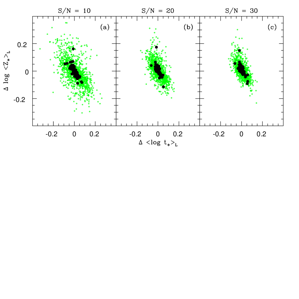
Figure 6: Output minus input residuals in $\log<Z_{\star}>_{L}$ against residuals in $<\log t_{\star}>_{L}$. Small circles are the individual test galaxies. Large filled circles mark the mean residuals for 20 perturbed versions of the same test galaxy. The anti-correlation illustrates the effect of the age-metallicity degeneracy.

Our method tends to underestimate $<Z_{\star}>$ for metal-rich systems and vice-versa. This bias is due to the infamous age-metallicity degeneracy. In order to verify to which degree our synthesis is affected by this well known problem (e.g., Renzini & Buzzoni 1986; Worthey 1994; Bressan, Chiosi & Tantalo 1996) we have examined the correlation between the output minus input residuals in $<\log t_{\star}>_{L}$ and $\log<Z_{\star}>_{L}$. The age-$Z$ degeneracy acts in the sense of confusing old, metal-poor systems with young, metal-rich ones and vice-versa, which should produce anti-correlated residuals. These are indeed seen in figure 6, where small symbols represent all 1300 individual simulations and filled circles correspond to the mean residuals obtained for each set of 20 perturbations of the 65 test galaxies. This anti-correlation is also present with the mass-weighted mean stellar metallicity $<Z_{\star}>_{M}$, but is not as strong as for $<Z_{\star}>_{L}$. On the other hand, the uncertainty in $<Z_{\star}>_{M}$ is always larger than for $<Z_{\star}>_{L}$ (Table 1).

The age-$Z$ degeneracy is thus present in our method, introducing systematic biases in our $<Z_{\star}>$ and $<\log t_{\star}>$ estimates at the level of up to $\sim 0.1$–0.2 dex. None of the results reported in this paper rely on this level of precision.

2.3 Simulations for random parameters

We have also carried out a separate set of simulations for 100 test galaxies generated by random combinations of $\vec{x}$, $A_{V}$, $\sigma_{\star}$. These simulations differ from the ones presented above in that the test galaxies are not restricted to match the range of properties inferred from the application of the synthesis to SDSS galaxies (Section 3). Given that these random galaxies span a broader (but less representative of our sample galaxies) region of the parameter space, one might expect to find larger uncertainties in the derived properties. This was indeed confirmed in the numerical experiments, although the effect is small. The uncertainties in the $(x_{Y},x_{I},x_{O})$ binned fractions increase by just a couple of percentage points with respect to those in Table 1. Similarly, the increase in $\Delta A_{V}$ is of just 0.02 mag, while $\Delta<\log t_{\star}>_{L}$ and $\Delta\log<Z_{\star}>_{M}$ increase by $\sim 0.02$ and 0.03 dex respectively.

The only properties whose uncertainties are substantially larger that those reported in Table 1 are the stellar mass and velocity dispersion. For instance, while the SDSS-based simulations for $S/N=10$ yield $\Delta\log M_{\star}=0.08$ dex and $\Delta\sigma_{\star}=12$ km s^-1, with random galaxies these errors increase to 0.15 dex and 24 km s^-1 respectively. The reason for this apparent discrepancy is due to the fact that the set of random test-galaxies contains a larger proportion of systems dominated by very young stellar populations than we find for SDSS galaxies. An error $\Delta x_{Y}$ in the light fraction associated to these populations must be compensated by errors in the older components, which carry most of the mass, even when $x_{Y}$ is large. As illustrated by the size of the error-bars in figure 4, $\Delta x_{Y}$ increases as $x_{Y}$ increases, so the errors in the mass fractions components increase too, leading to larger dispersion in $M_{\star}$. Furthermore, galaxies with large $x_{Y}$ have few absorption features to constrain the kinematical broadening of the spectrum, which explains the larger dispersion in our $\sigma_{\star}$ estimates. To prove this point, we have re-evaluated the uncertainties in $M_{\star}$ and $\sigma_{\star}$ excluding test galaxies with $x_{Y}>70$%, which corresponds to systems which formed $\ga 20$% of their stellar mass over the past $<10^{8}$ yr. For this subset of the simulations, which comprise 72 galaxies (each one split onto 20 different spectra corresponding to independent Monte Carlo realizations of the noise), the uncertainties in mass and velocity dispersion decrease to $\Delta\log M_{\star}=0.09$ dex and $\Delta\sigma_{\star}=14$ km s^-1 (for $S/N=10$), only slightly larger than those reported in Section 2.2.3. Uncertainties in other properties also decrease to values very similar to those listed in Table 1.

We thus conclude that the parameter uncertainties studied in Section 2.2 and summarized in Table 1 are only moderately affected by the design of the simulations, and represent fair estimates of the limitations of our synthesis method.

Finally, we have carried out simulations using the $Z=0.02Z_{\odot}$ BC03 SSPs to generate further test galaxies. Galaxies with such low metallicity are not expected to be present in significant numbers in the sample described in Section 3.1, given that it excludes low luminosity systems like HII galaxies and dwarf ellipticals (which are also the least metallic ones by virtue of the mass-metallicity relation). Still, it is interesting to investigate what would happen in this case. When synthesized with our 0.2–$2.5Z_{\odot}$ base (Fig. 1), these extremely metal poor galaxies are modeled predominantly with the $0.2Z_{\odot}$ components, as intuitively expected. Moreover, the mismatch in metallicity introduces non-negligible biases in other properties, like masses, mean ages and extinction ($M_{\star}$, for instance, is systematically underestimated by 0.3 dex). Similar problems should be encountered when modeling systems with $Z>2.5Z_{\odot}$. These results serve as a reminder that our base spans a wide but finite range in stellar metallicity, and that extrapolating these limits has an impact on the derived physical properties. While there is no straightforward a priori diagnostic of which galaxies violate these limits, in general, one should be suspicious of objects with mean $Z_{\star}$ too close to the base limits.

2.4 Summary of the simulations

Summarizing this theoretical study, we have performed simulations designed to evaluate the accuracy of our spectral synthesis method. The simulations mimic in as much as possible the wavelength range, spectral resolution, error spectrum, and $S/N$ of the actual SDSS data studied below. Several physically motivated combinations of the synthesis parameters were investigated to establish their precision at different $S/N$. Table 1 summarizes the uncertainties in these quantities and a few additional ones not explicitly mentioned above. In what follows we focus on 5 parameters: Stellar mass, velocity dispersion, extinction, mean stellar ages and metallicities, all of which were found to be adequately recovered.

This exercise demonstrates that we are capable of producing reliable estimates of several parameters of astrophysical interest, at least in principle. We must nevertheless emphasize that this conclusion relies entirely on models and on an admittedly simplistic view of galaxies. When applying the synthesis to real galaxy spectra, a series of other effects come into play. For instance, the extinction law appropriate for each galaxy likely differs from the one used here: in our Galaxy, the ratio of total to selective extinction of stellar sources, $R_{V}=A_{V}/E(B-V)$, is known to depend on the line of sight (Cardelli et al. 1989; Patriarchi et al. 2001); in addition, the wavelength dependence of the attenuation of light from an extended source such as a galaxy includes the effects of scattering back into the light beam, and depends on the relative distribution of stars and dust (Witt et al. 1992; Gordon et al. 1997). Also, one might expect that each population of stars is affected by a distinct extinction (Panuzzo et al. 2003; Charlot & Fall 2000). Similarly, while in the evolutionary tracks adopted here the metal abundances are scaled from the solar values, non-solar abundance mixtures are known to occur in stellar systems (e.g., Trager et al. 2000a,b), not to mention uncertainties in the SSP models and the always present issue of the IMF. In short, evidence against these simplifying hypothese abound.

Accounting for all these effects in a consistent way is not currently feasible. We mention these caveats not to dismiss simple models, but to highlight that all parameter uncertainties discussed above are applicable within the scope of the model. Hence, while the simulations lend confidence to the synthesis method, one might remain skeptical of its actual power. The next sections further address the reliability of the synthesis, this time from a more empirical perspective.

3 Analysis of a volume-limited galaxy sample

In this section we apply our synthesis method to a large sample of SDSS galaxies to estimate their stellar population properties. We also present measurements of emission line properties, obtained from the observed minus synthetic spectra. The information provided by the synthesis of so many galaxies allows one to address a long menu of astrophysical issues related to galaxy formation and evolution. Before venturing in the exploration of such issues, however, it is important to validate the results of the synthesis by as many means as possible. Hence, the goal of the study presented below is not so much to explore the physics of galaxies but to provide an empirical test of our synthesis method. The results reported in this section are used in Sections 4 and 5 with this purpose.

3.1 Sample definition

The spectroscopic data used in this work were taken from the SDSS. This survey provides spectra of objects in a large wavelength range (3800–9200 Å) with mean spectral resolution $\lambda/\Delta\lambda\sim 1800$, taken with 3 arcsec diameter fibers. The most relevant characteristic of this survey for our study is the enormous amount of good quality, homogeneously obtained spectra. The data analyzed here were extracted from the SDSS main galaxy sample available in the Data Release 2 (DR2; Abazajian et al. 2004). This flux-limited sample consists of galaxies with reddening-corrected Petrosian $r$-band magnitudes $r\leq 17.77$, and Petrosian $r$-band half-light surface brightnesses $\mu_{50}\leq 24.5$ mag arcsec^-2 (Strauss et al. 2002).

From the main sample, we first selected spectra with a redshift confidence $\geq 0.35$. Following the conclusions of Zaritsky, Zabludoff, & Willick (1995), we have imposed a redshift limit of $z>0.05$ (trying to avoid aperture effects and biases; see e.g. Gómez et al. 2003) and selected a volume limited sample up to $z=0.1$, corresponding to a $r$-band absolute magnitude limit of $M(r)=-20.5$. The absolute magnitudes used here are k-corrected with the help of the code provided by Blanton et al. (2003; kcorrect v3_2) and assuming the following cosmological parameters: $H_{0}$ = 70 km s^-1 Mpc^-1, $\Omega_{M}=0.3$ and $\Omega_{\Lambda}=0.7$. We also restricted our sample to objects for which the observed spectra show a $S/N$ ratio in $g$, $r$ and $i$ bands greater than 5. These restrictions leave us with a volume limited sample containing $50362$ galaxies, which leads to a completeness level of $\sim$ 98.5 per cent.

3.2 Results of the spectral synthesis

All 50362 spectra were brought to the rest-frame (using the redshifts in the SDSS database), sampled from 3650 to 8000 Å in steps of 1 Å, corrected for Galactic extinction using the maps given by Schlegel, Finkbeiner & Davis (1998) and the extinction law of Cardelli et al. (1989, with $R_{V}=3.1)$, and normalized by the median flux in the 4010–4060 Å region. The $S/N$ ratio in this spectral window spans the 5–30 range, with median value of 14. Besides the masks around the lines listed in Section 2.2.1, we exclude points with SDSS flag $\geq 2$, which signals bad pixels, sky residuals and other artifacts. After this pre-processing, the spectra are fed into the STARLIGHT code described in Section 2.1. On average, the synthesis is performed with $N_{\lambda}=3677$ points, after discounting the ones which are clipped by our $\leq 3$ sigma threshold (typically 40 points) and the masked ones.

The spectral fits are generally very good, as illustrated in Figs. 2 and 3. The mean value of $\chi^{2}/N_{\lambda}$ is 0.78. In fact, this is somewhat too good, since from the simulations we expect $\chi^{2}/N_{\lambda}\sim 0.95$. This is a minor difference, which could be fixed decreasing the errors in $O_{\lambda}$ by $\sim 10$%. We further quantify the quality of the fits by $\Delta_{\lambda}$, the mean value of $|O_{\lambda}-M_{\lambda}|/O_{\lambda}$ over all non-masked points. From the simulations we expect this alternative figure of merit to be of order of 0.6 times the noise-to-signal ratio at $\lambda_{0}$ (Table 1). This is exactly the mean value of $\Delta_{\lambda}\times S/N$ in the actual fits, again indicating acceptable fits.

The total stellar masses of the galaxies were obtained from the stellar masses derived from the spectral synthesis (which correspond to the light entering the fibers) by dividing them by $(1-f)$, where $f$ is the fraction of the total galaxy luminosity in the $z$-band outside the fiber. This approach, which neglects stellar population and extinction gradients, leads to an increase of typically 0.5 in $\log M_{\star}$. We did not apply any correction to the velocity dispersion estimated by the code given that the spectral resolution of the BC03 models and the data are very similar.

We point out that we did not constrain the extinction $A_{V}$ to be positive. There are several reasons for this choice: (a) some objects may be excessively dereddened by Galactic extinction; (b) some objects may indeed require bluer SSP spectra than those in the base; (c) the observed light may contain a scattered component, which would induce a bluening of the spectra not taken into account by the adopted pure extinction law; (d) constraining $A_{V}$ to have only positive values produces an artificial concentration of solutions at $A_{V}=0$, an unpleasant feature in the $A_{V}$ distribution. Interestingly, most of the objects for which we derive negative $A_{V}$ (typically $-0.1$ to $-0.3$ mag) are early-type galaxies. These galaxies are dominated by old populations, and expected to contain little dust. This is consistent with the result of K03, who find negative extinction primarily in galaxies with a large $D_{n}(4000)$. The distribution of $A_{V}$ for these objects, which can be selected on the basis of spectral or morphological properties, is strongly peaked around $A_{V}=0$, so that objects with $A_{V}<0$ can be considered as consistent with having zero extinction. In any case, none of the results reported in this paper is significantly affected by this choice.

3.3 Emission line measurements

Besides providing estimates of stellar population properties, the synthesis models allow the measurement of emission lines from the “pure-emission”, starlight subtracted spectra $(O_{\lambda}-M_{\lambda})$. We have measured the lines of [O ii]$\lambda\lambda$3726,3729, [O iii]$\lambda$4363, H$\beta$, [O iii]$\lambda\lambda$4959,5007, [O i]$\lambda$6300, [N ii]$\lambda$6548, H$\alpha$, [N ii]$\lambda$6584 and [S ii]$\lambda\lambda$6717,6731. Each line was treated as a Gaussian with three parameters: width, offset (with respect to the rest-frame central wavelength), and flux. Lines from the same ion were assumed to have the same width and offset. We have further imposed [O iii]$\lambda 5007$/[O iii]$\lambda 4959=2.97$ and [N ii]$\lambda 6584$/[N ii]$\lambda 6548=3$ flux ratio constraints. Finally, we consider a line to have significant emission if its fit presents a $S/N$ ratio greater than 3.

In some of the following analysis, galaxies with emission lines are classified according to their position in the [O iii]/H$\beta$ versus [N ii]/H$\alpha$ diagram proposed by Baldwin, Phillips & Terlevich (1981) to distinguish normal star-forming galaxies from galaxies containing active galactic nuclei (AGN). We define as normal star-forming galaxies those galaxies that appear in this diagram and are below the curve defined by K03 (see also Brinchmann et al. 2004). Objects above this curve are transition objects and galaxies containing AGN.

3.4 Aperture bias

A point that deserves mention here is the bias that may be introduced in the analysis due to the use of small fibers to measure the galaxy spectra. This effect, known as aperture bias, may introduce a redshift dependence in the measured galaxy spectra, since the fraction of galaxy light received by a fiber increases with increasing distance. Zaritsky et al. (1995), based on an analysis of spectra from the Las Campanas Redshift Survey, find that a lower limit on redshifts of $z=0.05$ minimizes the aperture bias. This effect has also been discussed by K03, Gómez et al. (2003) and Tremonti et al. (2004) for SDSS spectra. For instance, these authors found that the galaxy $z$-band $M/L$ ratio and the gas-phase oxygen abundance decrease by $\sim$ 0.1 dex over the redshift range of the survey, indicating that these quantities are moderately affected by aperture bias. The redshift range considered in our study is smaller than that of the entire survey, implying that the aperture effects are expected to be even smaller in our sample.

In order to verify whether our results are significantly affected by this bias, we investigated the behaviour of some of the quantities resulting from our analysis ($M_{\star}$, $<Z_{\star}>$, $<\log t_{\star}>$ and $A_{V}$) as a function of redshift for galaxies with luminosities above and below $M(r)=-21.17$, the median luminosity of our sample. We divided the sample in several redshift bins containing the same number of objects, and computed the median value and the quartiles of each quantity in each bin. Fig. 7 shows as solid lines the median values of each distribution, as well as their respective quartiles. None of the quantities seems to be strongly affected by this bias. The largest correlation with $z$ appears for light-weighted ages, corresponding to a change along our redshift distribution of about $0.1$ and $0.26$ dex for faint and bright galaxies, respectively. This is a plausible result since the light of nearby objects seen by the fiber aperture is dominated by the older stellar populations of their bulges. For the other quantities the variations are well below 0.1 dex.

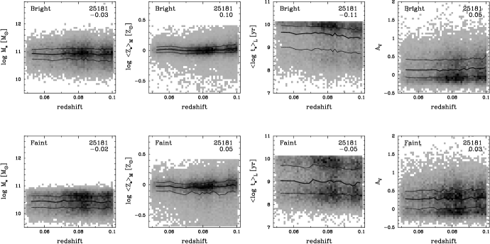
Figure 7: Trends of median values (and respective quartiles) of the stellar mass, mean stellar metallicity, mean stellar age and the V-band extinction as a function of redshift. Results are shown for galaxies with luminosities above (“Bright”, top panels) and below (“Faint”, bottom panels) the median luminosity of the sample. In this and following figures the gray scale level represents the number of galaxies in each pixel, darker pixels having more galaxies; the upper number in the top right of each panel indicates the total number of galaxies in the plot, and the lower one is the Spearman rank correlation coefficient ($r_{S}$).

4 Comparisons with the MPA/JHU database

The SDSS database has been explored by several groups, using different approaches and techniques. The MPA/JHU group has recently publicly released catalogues of derived physical properties for 211894 SDSS galaxies, including 33589 narrow-line AGN (K03, see also Brinchmann et al. 2004). These catalogues are based on the K03 method to infer the star formation histories, dust attenuation and stellar masses of galaxies from the simultaneous analysis of the 4000 Å break strength, $D_{n}(4000)$, and the Balmer line absorption index H$\delta_{A}$. These two indices are used to constrain the mean stellar ages of galaxies and the fractional stellar mass formed in bursts over the past few Gyr, and a comparison with broad-band photometry then allows to estimate the extinction and stellar masses.

The MPA/JHU catalogues provide very useful benchmarks for similar studies. In this section we compare the values of some of the parameters from these catalogues with our own estimates. Catalogues of galaxy properties obtained with our synthesis method will be made available in due course. Besides comparing directly measurements of physical quantities, our aim is also to highlight the differences that may appear due to the use of different methods and procedures.

4.1 Stellar extinction

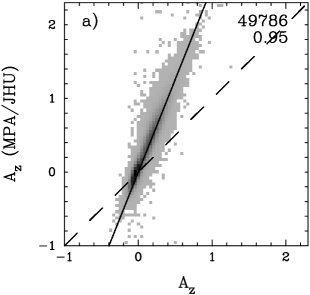
Figure 8: Comparison of the stellar extinction in the $z$-band determined by the MPA/JHU group with that estimated though the method described in this paper. The solid line shows a $y=ax$ linear fit to the data, while the dash ones is the identity line ($y=x$).

The MPA/JHU group estimates the $z$-band stellar extinction $A_{z}$ through the difference between model and measured colours, assuming an attenuation curve proportional to $\lambda^{-0.7}$. In our case, the extinction $A_{V}$ is derived directly from the spectral fitting, carried out with the Milky Way extinction law (Cardelli et al. 1989, c.f. Section 2.1), for which $A_{z}=0.4849A_{V}$ assuming $\lambda_{z}=8931$ Å. Fig. 8 shows that these two independent estimates are very strongly and linearly correlated, with a Spearman rank correlation coefficient $r_{S}=0.95$. However, the values of $A_{z}$ reported by the MPA/JHU group (column 17 of their Stellar Mass Catalogue) are systematically larger than our values: $A_{z}({\rm MPA/JHU})\simeq 2.51A_{z}({\rm This~{}Work})$ in the median.

This discrepancy is only apparent. The Galactic extinction law is substantially harder than $\lambda^{-0.7}$. One thus expects to need less extinction when modeling a given galaxy with the former law than with the latter. This was confirmed by STARLIGHT fits to a sub-set of SDSS galaxies using a $\lambda^{-0.7}$-law, which yield a value of $A_{V}$ typically 1.77 times larger than those obtained with the Cardelli et al. (1989) law. Since the $A_{z}/A_{V}$ conversion factors are 0.7030 and 0.4849 for the $\lambda^{-0.7}$ and Cardelli et al. laws, one finds that the $A_{z}$ values obtained for the two laws should differ by a factor of $1.77\times 0.7030/0.4849=2.57$. This is very close to the empirically derived factor of 2.51 (Fig. 8). We thus conclude that there are no substantial differences between the MPA/JHU and our estimates of the stellar extinction other than those implied by the differences in the reddening laws adopted in the two studies.

4.2 Stellar masses

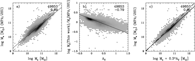
Figure 9: (a) Comparison of the stellar mass determined by the MPA/JHU group with our estimate. The solid line shows a $y=ax+b$ linear fit to the data, while the dash ones is the identity line ($y=x$). (b) Relation of the ratio between our and the MPA/JHU masses and our estimate of the V-band stellar extinction. (c) Comparison of the stellar masses after correcting for differences induced by the different extinction laws.

Fig. 9a compares our results for the total stellar masses to the MPA/JHU extinction-corrected stellar masses (column 9 of their Stellar Mass Catalogue). The two estimates of $M_{\star}$ correlate very well, with $r_{S}=0.89$. The quantitative agreement is also good, with a median difference of just 0.1 dex. This small offset cannot be attributed to the different IMFs employed in the two studies (Chabrier 2003 here and Kroupa 2001 in K03), since, as illustrated in figure 4 of BC03, these two IMFs yield practically identical $M/L$ ratios. Instead, this offset seems to be due to a subtle technicality. Whereas we adopt the $M/L$ ratio of the best $\chi^{2}$ model, the MPA/JHU group derives $M/L$ comparing the observed values of the $D_{n}(4000)$ and $H\delta_{A}$ indices with a library of 32000 models. Each model is then weighted by its likelihood, and a probability distribution for $M/L$ is computed. The MPA/JHU mass is the median of this distribution, which is not necessarily the same as the best-$\chi^{2}$ value. In fact, the Stellar Mass Catalogue of Brinchmann et al. (2004) lists in its column 8 the best $\chi^{2}$ masses, which are systematically larger than the median ones by $\sim 0.1$ dex, identical to the median difference identified above.

Part of the scatter in Fig. 9a can be attributed to the different extinction laws. Extinction contributes $+0.4A_{\lambda_{0}}$ to the estimated $\log M_{\star}$. As discussed above, using a $\lambda^{-0.7}$ law in the synthesis yields values of $A_{V}$ which are 1.77 times larger than using the Cardelli et al. (1989) law. Furthermore, the mass-to-light ratios obtained with the two laws are very similar. From this we expect that $\log M_{\star}({\rm This~{}Work})/M_{\star}(\rm MPA/JHU)\approx-0.3A_{V}({\rm This~{}Work})$, in good agreement with the observed relation (Fig. 9b). Correcting for this effect by adding $0.3A_{V}$ to our mass estimates indeed produces a better correlation, with $r_{S}=0.95$, as illustrated in Fig. 9c.

Overall, we conclude that the two mass estimates agree to within 0.4 dex. This level of agreement is similar to that recently found by Drory, Bender & Hopp (2004) in their comparison between the MPA/JHU masses and estimates based on SDSS plus 2MASS photometry. It is quite remarkable that, despite the substantial differences between our approaches and the underlying assumptions, the estimated stellar masses are so similar over a wide range of masses. On the other hand, this may not be so surprising given that the MPA/JHU group estimates of physical properties are ultimately based on a comparison of observed indices with an extensive library of galaxy spectra constructed out of the BC03 evolutionary synthesis models (K03). Since this library spans a wide of metallicities and star-formation histories, the agreement between our estimates and those of the MPA/JHU group may be simply indicating that the $N_{\star}=45$ SSPs from BC03 used in our spectral synthesis span a similar parameter-space to that covered by the K03 models.

4.3 Velocity dispersion

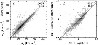
Figure 10: Comparison of the velocity dispersions (a) and oxygen abundances (b) determined by the MPA/JHU group with our estimates. The solid line shows a $y=ax+b$ linear fit to the data, while the dash ones is the identity line ($y=x$).

We use the sub-sample of galaxies with active nuclei to compare our measurements of absorption line broadening due to galaxy velocity dispersion and/or rotation, $\sigma_{\star}$, with those of the MPA/JHU group, since they list this quantity only in their AGN Catalogue (in column 16). The comparison is displayed in Fig. 10a. The Spearman correlation-coefficient in this case is $r_{S}=0.91$ and the median of the difference between the two estimates is just 9 km s^-1, indicating an excellent agreement between both studies.

4.4 Emission lines and nebular metallicities

Brinchmann et al. (2004) also provide, in their Emission line Catalogue, emission lines fluxes and equivalent widths which can be compared with our own measurements. In both studies the emission lines are measured after subtracting from the observed spectrum a model spectrum representing the stellar emission. In our case this is done with our synthesized spectra. The MPA/JHU group adopts a similar approach (see Tremonti et al. 2004 for a brief description) by fitting the observed continuum with BC03 models. They adopt, however a single metallicity model and a different extinction law. We have compared the fluxes and equivalent widths of H$\alpha$, [N ii]$\lambda 6584$, [O ii]$\lambda 3727$, H$\beta$ and [O iii]$\lambda 5007$ as measured by our code and that obtained by the MPA/JHU group. We do not find any significant difference between these values; the largest discrepancy ($\sim$ 5 per cent) was found for the equivalent widths of H$\alpha$ and [N ii], probably due to different estimates of the continuum level and the associated underlying stellar absorption. Our emission line measurements are also in good agreement with those in Stasińska et al. (2004), who fit the Balmer lines with emission and absorption components, instead of subtracting a starlight model.

In Fig. 10b we plot our estimates of the nebular oxygen abundance against those obtained by the MPA/JHU group (Catalogue of Gas Phase Metallicities, median values; see Tremonti et al. 2004). In order not to introduce any bias due to the use of different indicators of the oxygen abundance, we have estimated O/H using the calibration of the ([O ii]$\lambda$3726,3729 + [O iii]$\lambda$4959,5007)/ H$\beta$ ratio given by Tremonti et al. (2004) in their equation (1). This calibration is based on simultaneous fits of the most prominent emission lines with a model designed for the interpretation of integrated galaxy spectra (Charlot & Longhetti 2001). The oxygen abundances estimated in such a way differ by just $\sim 0.05$ dex, as shown in Fig. 10b.

Overall, we conclude that our spectral synthesis method yields estimates of physical parameters in good agreement with those obtained by the MPA/JHU group, considering the important differences in approach and underlying assumptions.

5 Empirical relations

Yet another way to assess the validity of physical properties derived through a spectral synthesis analysis is to investigate whether this method yields astrophysically reasonable results. In this section we follow this empirical line of reasoning by comparing some results obtained from our synthesis of SDSS galaxies (which excludes emission lines) with those obtained from a direct analysis of the emission lines. Our aim is to demonstrate that our synthesis results do indeed make sense. A more detailed discussion of most of the points below will be presented in other papers of this series.

5.1 Stellar and Nebular Metallicities

Our spectral synthesis approach yields estimates of the mean metallicity of the stars in a galaxy, $<Z_{\star}>$. The analysis of emission lines, on the other hand, gives estimates of the present-day abundances in the warm interstellar medium. Although stellar and nebular metallicities are not expected to be equal, it is reasonable to expect that they should roughly scale with each other.

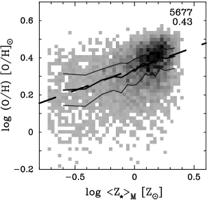
Figure 11: Nebular oxygen abundance versus mass-weighted stellar metallicity, both in solar units, for normal star-forming galaxies in our sample. The median values and quartiles in bins of same number of objects are shown as thin solid lines. The dashed line is a robust fit for the relation.

Fig. 11 shows the correlation between mass-weighted stellar metallicities and the nebular oxygen abundance (computed as in Section 4.4), both in solar units, for our sample of normal star-forming galaxies. A correlation is clearly seen, although with large scatter ($r_{S}=0.42$). Galaxies with large stellar metallicities also have large nebular oxygen abundances; galaxies with low stellar abundances tend to have smaller abundances. The observed scatter is qualitatively expected due to variations in enrichment histories among galaxies. A robust linear fitting gives the following relation:

$$\log\left(\frac{\mathrm{O/H}}{0.00049}\right)=0.34+0.23\log\left(\frac{<Z_{\star}>_{M}}{0.02}\right)$$ (7)

with a dispersion of 0.08 dex. Notice that in this expression both stellar and nebular metallicities are normalized to solar units ($Z_{\odot}=0.02$ and $(\mathrm{O/H})_{\odot}=0.00049$ respectively).

Nebular and stellar metallicities are estimated through completely different and independent methods, so the correlation depicted in Fig. 11 provides an a posteriori empirical validation for the stellar metallicity derived by the spectral synthesis. The possibility to estimate stellar metallicities for so many galaxies is one of the major virtues of spectral synthesis, as it opens an important window to study the chemical evolution of galaxies and of the universe as a whole (Panter et al. 2004; Sodré et al. in prep.).

5.2 Stellar and Nebular extinctions

The stellar extinction in the V-band is one of the products of our STARLIGHT code. A more traditional and completely independent method to evaluate the extinction consists of comparing the observed H$\alpha$/H$\beta$ Balmer decrement to the theoretical value. The intrinsic value of ${F({\rm H}\alpha)/F({\rm H}\beta)}$ is not very sensitive to the physical conditions of the gas, ranging from 3.03 for a gas temperature of 5000 K to 2.74 at 20000 K (Osterbrock 1989). Adopting a value of 2.86 for this ratio, the “Balmer extinction” (Stasińska et al. 2004) is given by

$$A_{V}^{\rm Balmer}=6.31\log\left[\frac{F({\rm H}\alpha)/F({\rm H}\beta)}{2.86}\right]$$ (8)

where the 6.31 coefficient comes from assuming the Cardelli et al. (1989) extinction curve.

Fig. 12 presents a comparison between the stellar $A_{V}$ and $A_{V}^{\rm Balmer}$. These two extinctions are determined in completely independent ways, and yet, our results show that they are closely linked, with $r_{S}=0.61$. A linear bisector fitting yields

$$A_{V}^{\rm Balmer}=0.24+1.81A_{V}$$ (9)

Note that the angular coefficient in this relation indicates that nebular photons are roughly twice as extincted as the starlight. This “differential extinction” is in very good qualitative and quantitative agreement with empirical studies (Fanelli et al. 1988; Calzetti, Kinney & Storchi-Bergmann 1994; Gordon et al. 1997; Mas-Hesse & Kunth 1999). We shall explore the implications of this result for the intrinsic colours of star-forming galaxies in another paper of this series (Stasińska et al. , in prep.).

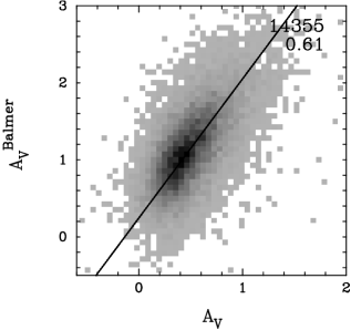
Figure 12: Relation between the nebular ($A_{V}^{\rm{Balmer}}$) and stellar ($A_{V}$) extinctions for our sample of normal star-forming galaxies. The solid line is a robust fit for the relation.

5.3 Relations with mean stellar age

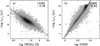
Figure 13: (a) Equivalent width of H$\alpha$ versus the light-weighted mean stellar age for normal emission line galaxies in our sample. (b) Relation between the D4000 index and the light-weighted mean stellar age. The solid lines are robust fits for the relations.

The equivalent width (EW) of H$\alpha$ is related to the ratio of present to past star formation rate of a galaxy (e.g., Kennicutt 1998). It is thus expected to be smaller for older galaxies. Fig. 13a shows the relation between EW(H$\alpha$) and the mean light-weighted stellar age obtained by our spectral synthesis. The anti-correlation, which has $r_{S}=-0.78$, is evident. From this plot we can derive an empirical relation which can be used to estimate $<\log t_{\star}>_{L}$ (for $\lambda_{0}=4020$ Å) of star-forming galaxies through the measurement of EW(H$\alpha$):

$$<\log t_{\star}>_{L}=10.10-1.30\log\mathrm{EW}(H\alpha)$$ (10)

for $t_{\star}$ in yr and EW(H$\alpha$) in Å. It is worth stressing that these two quantities are obtained independently, since the spectral synthesis does not include emission lines.

Another quantity that is considered a good age indicator, even for galaxies without emission lines, is the 4000 Å break, D4000. We measured this index following Bruzual (1983), who define D4000 as the ratio between the average value of $F_{\nu}$ in the 4050–4250 and 3750–3950 Å bands. The relation between $<\log t_{\star}>_{L}$ and D4000 is shown in Fig. 13b. Note that the concentration of points at the high age end reflects the upper age limit of the base adopted here, 13 Gyr (c.f. Section 2.2.1). The correlation is very strong ($r_{S}=0.94$), showing that indeed D4000 can be used to estimate empirically mean light-weighted galaxy ages, despite its metallicity dependence for very old stellar populations (older than 1 Gyr, as shown by K03). From the tight relation between $<\log t_{\star}>_{L}$ and D4000 we derive the following empirical relation

$$<\log t_{\star}>_{L}=6.76+9.41\log{\mathrm{D}}4000$$ (11)

where $t_{\star}$ is in yr. This robust fit reproduces $<\log t_{\star}>_{L}$ to within an rms dispersion of 0.15 dex.

5.4 $M_{\star}$–$\sigma_{\star}$ relation

Fig. 14 shows the relation between stellar mass and $\sigma_{\star}$, obtained from the synthesis. The relation is quite good, with $r_{S}=0.79$. The solid line displayed in the figure is

$$\log M_{\star}=6.44+2.04\log\sigma_{\star}$$ (12)

for $M_{\star}$ in $M_{\odot}$ and $\sigma_{\star}$ in km s^-1, obtained with a bisector fitting. The figure also shows as a dashed line a fit assuming $M_{\star}\propto\sigma_{\star}^{4}$, expected from the virial theorem under the (unrealistic) assumption of constant mass surface density. In both cases we have excluded from the fit galaxies with $\sigma_{\star}<35$ km s^-1, which corresponds to less than half the spectral resolution of both data and models.

This is another relation that is expected a priori if we have in mind the Faber-Jackson relation for ellipticals and the Tully-Fisher relation for spirals. For early-type galaxies, $\sigma_{\star}$ is a measure of the central velocity dispersion, which is directly linked to the gravitational potential depth, and, through the virial theorem, to galactic mass. For late-type systems, $\sigma_{\star}$ has contributions of isotropic motions in the bulges, as well as of the rotation of the disks, and is also expected to relate with galactic mass. Another aspect that it is interesting to point out in Fig. 14 is that the dispersion in the $M_{\star}$–$\sigma_{\star}$ relation decreases as we go from low-luminosity, rotation-dominated systems, for which the values of $\sigma_{\star}$ depend on galaxy inclination and bulge-to-disk ratio, to high-luminosity, mostly early-type systems, which obey a much more regular (and steeper) relation between $\sigma_{\star}$ and $M_{\star}$.

This relation, between a quantity that is not directly linked to the synthesis, $\sigma_{\star}$, and another one that is a product of our synthesis, $M_{\star}$, is yet another indication that the results of our STARLIGHT code do make sense.

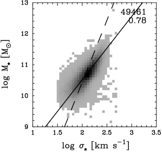
Figure 14: Mass-velocity dispersion relation for our sample. The solid line is a robust fit for the data while dashed one is a fitting assuming $M_{\star}\propto\sigma^{4}$.

6 Summary

We have developed and tested a method to fit galaxy spectra with a combination of spectra of individual simple stellar populations generated with state-of-the art evolutionary synthesis models. The main goal of this investigation was to examine the reliability of physical properties derived in this way. This goal was pursued by three different means: simulations, comparison with independent studies, and analysis of empirical results. Our main results can be summarized as follows:

1. Simulations tailored to match the characteristics of SDSS spectra show that the individual SSP strengths, encoded in the population vector $\vec{x}$, are subjected to large uncertainties, but robust results can be obtained by compressing $\vec{x}$ into coarser but useful indices. In particular, physically motivated indices such as mean stellar ages and metallicities are found to be well recovered by spectral synthesis even for relatively noisy spectra. Stellar masses, velocity dispersion and extinction are also found to be accurately retrieved.

2. We have applied our STARLIGHT code to a volume limited sample of over 50000 galaxies from the SDSS Data Release 2. The spectral fits are generally very good, and allow accurate measurements of emission lines from the starlight subtracted spectrum. Catalogues of physical and emission line properties derived for this sample will be made available in due course. We also report that work is underway to produce a flexible, user friendly and publicly available version of STARLIGHT.

3. We have compared our results to those obtained by the MPA/JHU group (K03; Brinchmann et al. 2004) with a different method to characterize the stellar populations of SDSS galaxies. The stellar extinctions and masses derived in these two studies are very strongly correlated. Furthermore, differences in the values of $A_{V}$ and $M_{\star}$ are found to be mostly due to the differences in the model ingredients (extinction law). Our estimates of stellar velocity dispersions and emission line properties are also in good agreement with those of the MPA/JHU group.

4. The confidence in the method is further strengthened by several empirical correlations between synthesis results and independent quantities. We find strong correlations between stellar and nebular metallicites, stellar and nebular extinctions, mean stellar age and the equivalent width of H$\alpha$, mean stellar age and the 4000 Å break, stellar mass and velocity dispersion. These are all astrophysically reasonable results, which reinforce the conclusion that spectral synthesis is capable of producing reliable estimates of physical properties of galaxies.

Overall, these results validate spectral synthesis as a powerful tool to study the history of galaxies. Other papers in this series will take advantage of this tool to address issues regarding aspects of galaxy formation and evolution.

References

- [] Abazajian, K., et al. 2003, AJ, 126, 2081
- [] Abazajian K. et al. 2004, AJ, 128, 502
- [] Allende Prieto C., Lambert D. L., Asplund M., 2001, ApJ, 556, L63
- [] Arimoto, N. & Yoshii, Y. 1987, A&A, 173, 23
- [] Baldwin J. A., Phillips M. M., & Terlevich R., 1981, PASP, 93, 5
- [] Balogh M., Morris S., Yee H., et al. , 1999, ApJ, 527, 54
- [] Bertone, E., Buzzoni, A., Rodríguez-Merino, L. H., & Chávez, M. 2004, Memorie della Societa Astronomica Italiana, 75, 158
- [] Bica E., 1988, A&A, 195, 76
- [] Blanton M. R, Brinkmann J., Csabai I., Doi M., Eisenstein D., Fukugita M., Gunn J. E., Hogg D. W., Schlegel D. J., 2003, AJ, 125, 2348
- [] Bressan A., Chiosi C., Tantalo R., 1996, A&A, 311, 425
- [] Brinchmann J., Charlot S., White S. D. M., Tremonti C., Kauffmann G., Heckman T., Brinkmann J., 2004, MNRAS, 351, 1151
- [] Bruzual G., 1983, ApJ, 273, 105
- [] Bruzual G., Charlot S., 2003, MNRAS, 344, 1000
- [] Cardelli J. A., Clayton G. C., Mathis J.S., 1989, ApJ, 345, 245
- [] Cardiel, N., Gorgas, J., Sánchez-Blázquez, P., Cenarro, A. J., Pedraz, S., Bruzual, G., & Klement, J. 2003, A&A, 409, 511
- [] Calzetti D., Kinney A. L., Storchi-Bergmann T., 1994, ApJ, 429, 582
- [] Chabrier G., 2003, PASP, 115, 763
- [] Charlot S., Longhetti M., 2001, MNRAS, 323, 887
- [] Charlot, S. & Fall, S. M. 2000, ApJ, 539, 718
- [] Cid Fernandes R., Sodré L., Schmitt H. R., Leão J.R. S., 2001, MNRAS, 325, 60
- [] Cid Fernandes R., Leao J. Lacerda R. R., 2003, MNRAS, 340, 29
- [] Cid Fernandes R., Gu Q., Melnick K., Terlevich E., Terlevich R., Kunth D. Rodrigues Lacerda R., Joguet B. 2004a, MNRAS, in press.
- [] Cid Fernandes R., González Delgado R., Storchi-Bergmann, T., Pires Martins, L., Schmitt H., 2004b, MNRAS, in press.
- [] Drory N., Bender R., Hopp U., 2004, ApJ, 616, L103
- [] Faber, S. M. 1972, A&A, 20, 361
- [] Fanelli, M.N., O’Connell, R.W., Thuan, T.X., 1988, ApJ 334, 665
- [] Fioc, M. & Rocca-Volmerange, B. 1997, A&A, 326, 950
- [] Garcia-Rissman et al. 2005, in prep.
- [] Gómez P.L. et al. , 2003, ApJ, 584, 210
- [] González Delgado, R. M.et al. 2004, MNRAS, submitted
- [] Gordon, K. D., Calzetti, D., & Witt, A. N. 1997, ApJ, 487, 625
- [] Guiderdoni, B. & Rocca-Volmerange, B. 1987, A&A, 186, 1
- [] Heavens, A. F., Jimenez, R., & Lahav, O. 2000, MNRAS, 317, 965
- [] Heavens, A., Panter, B., Jimenez, R., & Dunlop, J. 2004, Nature, 428, 625
- [] Jimenez, R., MacDonald, J., Dunlop, J. S., Padoan, P., & Peacock, J. A. 2004, MNRAS, 349, 240
- [] Kauffmann G. et al. , 2003, MNRAS, 341, 33
- [] Kennicutt R. C. Jr., 1998, ARA&A, 36, 189
- [] Kewley, L. J., Dopita, M. A., Sutherland, R. S., Heisler, C. A., & Trevena, J. 2001, ApJ, 556, 121
- [Kroupa(2001)] Kroupa, P. 2001, MNRAS, 322, 231
- [] Le Borgne J.-F. et al. , 2003, A&A, 402, 433
- [] Le Borgne, D., Rocca-Volmerange, B., Prugniel, P., Lançon, A., Fioc, M., & Soubiran, C. 2004, A&A, 425, 881
- [] Leitherer, C., Robert, C., & Heckman, T. M. 1995, ApJS, 99, 173
- [] Loveday, J., Peterson, B. A., Maddox, S. J., Efstathiou, G., 1996, ApJS, 107, 201
- [] Mas-Hesse, J. M. & Kunth, D. 1991, A&AS, 88, 399
- [] Mas-Hesse, J. M., & Kunth, D. 1999, A&AS, 349, 765
- [] MacKay, D. J. C. 2003, “Information Theory, Inference and Learning Algorithms”, Cambridge University Press.
- [] Moultaka J., Pelat D., 2000, MNRAS, 314, 409
- [] Morgan, W. W. 1956, PASP, 68, 509
- [] Moultaka, J., Boisson, C., Joly, M., & Pelat, D. 2004, A&A, 420, 459
- [] Osterbrock, D. E. 1989, Astrophysics of gaseous nebulae and active galactic nuclei (University Science Books)
- [] Patriarchi, P., Morbidelli, L., Perinotto, M., Barbaro, G, 2001, A&A, 372, 644
- [] Panter, B., Heavens, A. F., & Jimenez, R. 2004, MNRAS, 458
- [] Panuzzo P., Bressan A., Granato G. L., Silva L., Danese, L. 2003, A&A, 409, 99
- [] Pelat D., 1997, MNRAS, 284, 365
- [Prugniel & Soubiran(2001)] Prugniel, P. & Soubiran, C. 2001, A&A, 369, 1048
- [] Reichardt, C., Jimenez, R., & Heavens, A. F. 2001, MNRAS, 327, 849
- [] Renzini A., Buzzoni A., 1986, in Chiosi C., Renzini A., eds, Spectral Evolution of Galaxies. Riedel, Dordecht, p. 213
- [] Ronen, S., Aragon-Salamanca, A., & Lahav, O. 1999, MNRAS, 303, 284
- [] Schaerer, D. & Vacca, W. D. 1998, ApJ, 497, 618
- [] Schlegel D. J., Finkbeiner D. P., Davis M., 1998, ApJ, 500, 525
- [] Schmidt, A. A., Copetti, M. V. F., Alloin, D., & Jablonka, P. 1991, MNRAS, 249, 766
- [] Slosar, A., & Hobson, M. astro-ph/0307219
- [] Spinrad, H. & Taylor, B. J. 1972, Apj, 171, 397
- [] Stasińska G., Mateus A., Sodré L., Szczerba R., 2004, A&A, 420, 475
- [] Stoughton C. et al., 2002, AJ, 123, 485
- [] Strauss, M. A., et al. 2002, AJ, 124, 1810
- [] Tinsley, B. M. 1968, Apj, 151, 547
- [] Trager, S. C., Faber, S. M., Worthey, G., Jesús González, J. 2000a, ApJ, 119, 1645
- [] Trager, S. C., Faber, S. M., Worthey, G., Jesús González, J. 2000b, ApJ, 120, 165
- [] Tremonti C., 2003, PhD thesis, Johns Hopkins University
- [] Tremonti, C. A. et al., 2004, ApJ, in press (astro-ph/045537)
- [] Vazdekis, A. 1999, ApJ, 513, 224
- [] Vazdekis, A. & Arimoto, N. 1999, ApJ, 525, 144
- [] Witt, A.N., Thronson, H.A., Capuano J.M., 1992, ApJ 393, 611
- [] Wood, D. B. 1966, Apj, 145, 36
- [] Worthey G., 1994, ApJS, 94, 687
- [] York, D. G., et al. 2000, AJ, 120, 1579
- [] Zaritsky D., Zabludoff A. I., Willick J. A., 1995, AJ, 110, 1602