Cluster mergers and non-thermal phenomena : a statistical magneto–turbulent model

Abstract

There is now firm evidence that the ICM consists of a mixture of hot plasma, magnetic fields and relativistic particles. The most important evidences for non-thermal phenomena in galaxy clusters comes from the spectacular synchrotron radio emission diffused over Mpc scale observed in a growing number of massive clusters and, more recently, in the hard X–ray tails detected in a few cases in excess of the thermal bremmstrahlung spectrum. A promising possibility to explain giant radio halos is given by the presence of relativistic electrons reaccelerated by some kind of turbulence generated in the cluster volume during merger events. With the aim to investigate the connection between thermal and non–thermal properties of the ICM, in this paper we develope a statistical magneto-turbulent model which describes in a self-consistent way the evolution of the thermal ICM and that of the non-thermal emission from clusters. Making use of the extended Press & Schechter formalism, we follow cluster mergers and estimate the injection rate of the fluid turbulence generated during these energetic events. We then calculate the evolution of the spectrum of the relativistic electrons in the ICM during the cluster life by taking into account both the electron–acceleration due to the merger–driven turbulence and the relevant energy losses of the electrons. We end up with a synthetic population of galaxy clusters for which the evolution of the ICM and of the non–thermal spectrum emitted by the accelerated electrons is calculated. The generation of detectable non–thermal radio and hard X–ray emission in the simulated clusters is found to be possible during major merger events for reliable values of the model parameters. In addition the occurrence of radio halos as a function of the mass of the parent clusters is calculated and compared with observations. In this case it is found that the model expectations are in good agreement with observations: radio halos are found in about 30% of the more massive clusters in our synthetic population ($M$ $>$$\sim$ $1.8\times 10^{15}$ M_⊙) and in about 4% of the intermediate massive clusters ($9\times 10^{14}<M<1.8\times 10^{15}M_{\odot}$), while the radio halo phenomenon is found to be extremely rare in the case of the smaller clusters.

1 Introduction

1.1 Evidence for non-thermal phenomena

There is now firm evidence that the ICM is a mixture of hot gas, magnetic fields and relativistic particles.

The most important evidence for relativistic electrons in clusters of galaxies comes from the diffuse synchrotron radio emission observed in a growing number of massive clusters. The diffuse emissions are referred to as radio halos and/or radio mini–halos when they appear confined to the center of the cluster, while they are called relics when they are found in the cluster periphery (e.g., Feretti, 2003).

Diffuse radio emission is not the only evidence of non-thermal activity in the ICM. Additional evidence, comes from the detection of hard X-ray (HXR) excess emission in the case of the Coma cluster, A2256 and possibly A754 (Fusco–Femiano et al., 1999, 2000,03,04; Rephaeli et al., 1999; Rephaeli & Gruber, 2002,03). If these excesses are indeed of non-thermal origin, they may be explained in terms of IC scattering of relativistic electrons off the photons of the cosmic microwave background (CMB) (Fusco–Femiano et al., 1999,2000; Rephaeli et al., 1999; Völk & Atoyan 1999; Brunetti et al.2001a; Petrosian 2001; Fujita & Sarazin 2001; Blasi 2001). Unfortunately the poor sensitivity of the present and past HXR-facilities does not allow to obtain a iron-clad detection of these excesses and thus future observatories (e.g. ASTRO-E2, NEXT) are necessary to definitely confirm them (see Rossetti & Molendi 2004; Fusco-Femiano et al.2004), to constrain their spectral shape, and hopefully to increase the statistics of HXR excesses.

The presence of high energy hadrons is at present not yet proven, but in principle, due to confinement of cosmic rays over cosmological time scales (e.g., Völk et al. 1996; Berezinsky, Blasi & Ptuskin 1997), the hadron content of the intracluster medium might be appreciable and may be constrained by future gamma–ray observations (e.g., Blasi 2003; Miniati 2003).

1.2 Thermal – non-thermal connection

Giovannini, Tordi and Feretti (1999) found that $\sim$5% of clusters in a complete X-ray flux limited sample (from Ebeling et al.1996) have a radio halo source. The detection rate of radio halos shows an abrupt increase with increasing the X-ray luminosity of the host clusters. Indeed it has been found that about 30-35% of the galaxy clusters with X-ray luminosity larger than 10⁴⁵ erg s^-1 show diffuse non-thermal radio emission (Giovannini & Feretti 2002). The high luminosity of clusters hosting radio halos implies that these clusters also have a high temperature ($kT$ $>$ $\sim$$7$ keV) and a large mass ($>$ $\sim$$10^{15}$ M_⊙). Although still based on relatively poor statistics, these observations suggest a leading role of the cluster mass and/or temperature in the formation of radio halos.

In addition correlation between the radio power of radio halos at 1.4 GHz and the bolometric X–ray luminosity, temperature and mass of the parent clusters have been found (Colafrancesco 1999; Liang et al. 2000; Giovannini & Feretti 2002; Govoni et al.2001).

1.3 Models

The difficulty in explaining the extended radio halos arises from the combination of their $\sim$Mpc size, and the relatively short radiative lifetime of the radio emitting electrons. Indeed, the diffusion time necessary for the radio electrons to cover such distances is orders of magnitude larger than their radiative lifetime. As proposed first by Jaffe (1977), a solution to this puzzle would be provided by continuous in situ reacceleration of the relativistic electrons.

An alternative to the reacceleration scenario is given by secondary models, which were first put forward by Dennison (1980), who suggested that relativistic electrons may be produced in situ by inelastic proton-proton collisions through production and decay of charged pions.

There is now increasing evidence that present radio data, i.e. the fine radio properties of the radio halos and the halo–occurence, may be naturally accounted for by primary electron models whereas they may be difficult to be reproduced by secondary models (Brunetti, 2003; Kuo et al., 2004).

• In the framework of primary electron models, merger shocks can accelerate relativistic electrons to produce large scale synchrotron radio emission (e.g., Roettiger et al., 1999; Sarazin 1999; Takizawa & Naito, 2000; Blasi 2001). However, the radiative life–time of the emitting electrons diffusing away from these shocks is so short that they would just be able to produce relics and not Mpc sized spherical radio halos (e.g., Miniati et al, 2001). In addition, a number of papers (Gabici & Blasi 2003; Berrington & Dermer 2003) have recently pointed out that the Mach number of the typical shocks produced during major merger events is too low to generate non–thermal radiation with the observed fluxes, spectra and statistics.

• Re–acceleration of a population of relic electrons by turbulence diffused in the cluster volume and powered by major mergers is suitable to explain the very large scale of the observed radio emission and is also a promising possibility to account for the fine radio structure of the diffuse emission (Schlickeiser et al.1987; Brunetti et al., 2001a,b). In this framework, based on relatively simple assumptions, Ohno, Takizawa and Shibata (2002), and Fujita, Takizawa and Sarazin (2003) developed specific magneto-turbulent models for Alfvénic electron acceleration in galaxy clusters. More recently, Brunetti et al.(2004) presented the first self-consistent and time-dependent model for the interaction of Alfvén waves, relativistic electrons, thermal and relativistic protons in galaxy clusters. These authors proved that, under some physical conditions, radio halos and HXR tails may be activated by electron acceleration due to MHD waves injected during cluster merger events.

1.4 Why a statistical model ?

So far two works have investigated the statistics of the formation of radio halos from a theoretical point of view.

Enßlin and Röttgering (2002) calculated the radio luminosity function of cluster radio halos (RHLF). In a first modelling, they obtained RHLF by combining the X-ray cluster luminosity function with the radio–halo luminosity – X–ray luminosity correlation, assuming that a fraction, $f_{rh}\simeq\frac{1}{3}$, of galaxy cluster have radio halos. Then, in a slightly more accurate modelling, $f_{rh}$ was assumed to be equal to the fraction of clusters that have recently undergone a strong mass increase and the radio halo luminosity of a cluster was assumed to scale with $(1+z)^{-4}$ (due to the incresing IC-losses).

In a more recent paper, Kuo et al. (2004) calculated the formation rate and the comoving number density of radio halos in the hierarchical clustering scheme. The model was based on two morphological criteria to define the conditions necessary to the formation of radio halos : 1) the cluster mass must be greater than or equal to a threshold mass adjusted to observations (Giovannini et al. 1999); 2) the merger process must be violent enough to distrupt the cluseter core, and thus the relative mass increase was required to be $\Delta_{m}\equiv(\Delta M/M)_{th}=0.6$ according to numerical simulations (Salvador-Solè et al. 1998). Given the above criteria and making use of the Press-Shechter formalism these authors found that a duration of the radio halo phenomenon of the order of 1 Gyr would result to be in good agreement with the observed probability of formation of radio halos with the mass of the parent clusters.

As already pointed out, all these approaches are based on assumptions in defining the conditions of formations of radio halos based on observational correlations and/or mass thresholds. On the other hand, no effort has been done so far to model the formation of radio halos and HXR tails in a self–consistent approach, i.e. an approach which should model, at the same time, the evolution of the thermal properties of the ICM of the host galaxy clusters and the generation and evolution of the non–thermal phenomena.

As mentioned above, one of the ideas that is producing the most promising results for the interpretation of non–thermal phenomena in galaxy clusters consists in the magneto-turbulent re–acceleration of relic relativistic electrons leftover of the past activity occurred within the ICM.

The aim of this paper is thus to obtain a basic modelling of the statistical properties of radio halos and HXR tails in the above self–consistent approach in the framework of the magneto-turbulent re–acceleration scenario.

In order to have a straightforward comparison with published observational constraints, an Einstein de Sitter (EdS) model ($H_{o}=50$ km s^-1Mpc^-1, $q_{o}=0.5$) is assumed in the paper. In the Appendix A the results are also compared with those obtained in a $\Lambda$-CDM model.

2 The statistical magneto-turbulent Model: Outline

In this Section we outline the formalism and procedures used to develope our statistical model. The major steps can be sketched as follows :

• Cluster formation: The evolution and formation of galaxy clusters is computed making use of a semi–analytic procedure based on the hierarchical Press & Schechter 1974 (PS) theory of cluster formation. Given a present day mass and temperature of the parent clusters, the cosmological evolution (back in time) of the cluster properties (merger trees) are obtained making use of Monte Carlo simulations. A suitable large number of trees allows us to describe the statistical cosmological evolution of galaxy clusters.

• Turbulence in Galaxy Clusters: The turbulence in galaxy clusters is supposed to be injected during cluster mergers.

  The energetics of the turbulence injected in the ICM is calibrated with the $PdV$ work done by the infalling subclusters in passing through the volume of the most massive one; it basically depends on the density of the ICM and on the velocity between the two colliding subclusters. The sweaped volume in which turbulence is injected is estimated from the Ram Pressure Stripping (e.g., Sarazin 2002 and ref. therein). We assume that a relatively large fraction of the turbulence developed during these mergers is in the form of fast magneto–acoustic waves (MS waves). We use these waves since their damping rate and time evolution basically depend on the properties of the thermal plasma which are provided by our merger trees for each simulated cluster.

  The spectrum of the MS waves depends on many unknown quantities thus we adopt two extreme scenarios : the first one assumes a broad band injection of MHD waves (Sect. 4.2), the second one assumes that turbulence is injected at a single scale (Appendix B). In both cases the spectrum of MS waves is calculated solving a turbulent-diffusion equation in the wavenumber assuming that the turbulence, injected in the cluster volume for each merger event, is injected for- and thus dissipated in a dynamical crossing time.

• Particle Acceleration: We focus on the electron component only because the major damping of MS waves (which determines the spectrum of these waves and thus the efficiency of the particle acceleration, Sect. 5.2) is due to thermal electrons and thus hadrons cannot significantly affect the electron–acceleration process (see Sect.5.2.2). We assume a continuous injection of relativistic electrons in the ICM due to AGNs and/or Galactic Winds. At each time step, given the spectrum of MS waves and the physical conditions in the ICM, we compute the time evolution of relativistic electrons by solving a Fokker-Planck equation including the effect of electron acceleration due to the coupling between MS waves and particles, and the relevant energy losses.

Given a population of galaxy clusters by combining i)-iii) we are thus able to follow in a statistical way the cosmological evolution of the spectrum of the relativistic electrons in the volume of these clusters and the properties of the thermal ICM.

3 Cluster formation: PS formalism and a Monte Carlo approach

3.1 PS formalism and Merger rate

The PS theory assumes that galaxy clusters form hierarchically via mergers of subclusters which develope by gravitational instability of initially small amplitude Gaussian density fluctuations generated in the early Universe. Making use of the PS formalism, it is possible to obtain the probability that a “parent” cluster of mass $M_{1}$ at a time $t_{1}$ had a progenitor of mass in the range $M_{2}\rightarrow M_{2}+dM_{2}$ at some earlier time $t_{2}$, with $M_{1}>M_{2}$ and $t_{1}>t_{2}$. This is given by (e.g., Lacey & Cole 1993, Randall, Sarazin & Ricker 2002):

$${\cal P}(M_{2},t_{2}|M_{1},t_{1})dM_{1}=\frac{1}{\sqrt{2\pi}}\frac{M_{1}}{M_{2}}\frac{\delta_{c2}-\delta_{c1}}{(\sigma_{2}^{2}-\sigma_{1}^{2})^{3/2}}\left|\frac{d\sigma_{2}^{2}}{dM_{2}}\right|\times$$

$$\exp\left[-\frac{(\delta_{c2}-\delta_{c1})^{2}}{2(\sigma_{2}^{2}-\sigma_{1}^{2})}\right]dM_{2}\,,$$ (1)

where $\delta_{c}(z)$ is the critical linear overdensity for a region to collapse at a redshift $z$; for the EdS model it is given by:

$$\delta_{c}(t)=\frac{3(12\pi)^{2/3}}{20}\big{(}\frac{t_{0}}{t}\big{)}^{2/3}$$ (2)

with $t_{0}$ the present time, $\sigma(M)$ is the rms density fluctuation within a sphere of mean mass $M$. In Eq. (1) it is $\delta_{c1}\equiv\delta_{c}(t=t_{1})$ and $\sigma_{1}\equiv\sigma(M_{1})$, with similar definitions for $\delta_{c2}$ and $\sigma_{2}$. The standard deviation of matter density fluctuations at the smoothing scale R ($\sigma(M)$) is given by (e.g., Peebles, 1980):

$$\sigma(M)=\frac{1}{(2\pi)^{3}}\int P_{f}(k)\hat{W}^{2}(kR_{M})d^{3}k$$ (3)

where $\hat{W}^{2}(kR_{M})$ is the Fourier transform of the window function, the scale $R_{M}$ is chosen to contain a mass $M$, and $P(k)$ is the matter power spectrum at a given redshift that can be expressed as:

$$P_{f}(k)=P_{i}(k)T^{2}(k;z_{f})\bigg{[}\frac{D(z_{f})}{D(z_{i})}\bigg{]}^{2}\propto k^{n}T^{2}(k;z_{f})\bigg{[}\frac{D(z_{f})}{D(z_{i})}\bigg{]}^{2}$$ (4)

where $n$ is the spectral index of the primordial power spectrum $P_{i}(k)\propto k^{n}$; $T(k)$ is the ‘transfer function’ which transfer the initial perturbation to the present epoch and $D(z)$ is the growth factor of the linear perturbation. Over the range scales of our interest it is sufficient to consider a power-law spectrum of the density perturbation given by (Randall, Sarazin & Ricker 2002):

$$\sigma(M)=\sigma_{8}\,\left(\frac{M}{M_{8}}\right)^{-\alpha}\,,$$ (5)

where $\sigma_{8}$ is the present epoch rms density fluctuation on a scale of 8 $h^{-1}$ Mpc, and $M_{8}=(4\pi/3)(8\,h^{-1}\,{\rm Mpc})^{3}\bar{\rho}$ is the mass contained in a sphere of radius 8 $h^{-1}$ Mpc ($\overline{\rho}$ is the present epoch mean density of the Universe). The exponent in Eq.(5) is given by (Bahcall & Fan 1998) $\alpha=(n+3)/6$, $n$ being the slope of the power spectrum of the fluctuations. Following Randall, Sarazin & Ricker (2002), it is $\sigma_{8}=0.514$ for the EdS models.

It is convenient (Lacey & Cole 1993) to replace the mass $M$ and time $t$ (or redshift $z$) with the suitable variables $S\equiv\sigma^{2}(M)$ and $x\equiv\delta_{c}(t)$. With these definitions, $S$ decreases as the mass $M$ increases, and $x$ decreases with increasing cosmic time $t$.

Let $K(\Delta S,\Delta x)\,d\Delta S$ be the probability that a cluster had a progenitor with a mass corresponding to a change in $S$ of $\Delta S=\sigma_{2}^{2}-\sigma_{1}^{2}$ in the range $\Delta S\rightarrow\Delta S+d\Delta S$ at an earlier time corresponding to $\Delta x=\delta_{c2}-\delta_{c1}$. Then, from Eq.(1) one has :

$$K(\Delta S,\Delta x)d\Delta S=\frac{1}{\sqrt{2\pi}}\frac{\Delta x}{(\Delta S)^{3/2}}\exp\left[-\frac{(\Delta x)^{2}}{2\Delta S}\right]d\Delta S\,.$$ (6)

Figure 1: Comulative probability distribution ${\cal P}(<\Delta S,\Delta x)$ as a function of $log(\Delta S)$.

3.2 Monte Carlo Technique and Merger Trees

Following a relatively standard procedure adopted in the literature (e.g., Randall et al., 2002; Gabici & Blasi 2003), we employ a Monte Carlo technique to construct merger trees. Each tree starts at the present time with a cluster of mass $M$ and temperature $T$. We step each simulated cluster back in time, using a small but finite time step corresponding to a positive increase $\Delta x$. The step size determines the value of the minimum mass increment of the cluster, $\Delta M_{c}$, which is due essentially to a single merger event (Lacey & Cole 1993) :

$$(\Delta x)^{2}\la\left|{{d\ln\sigma^{2}}\over{d\ln M}}\right|\left({{\Delta M_{c}}\over{M}}\right)S\,,$$ (7)

where $M$ is the mass of the cluster at the current time step. The value $\Delta M_{c}$ gives the mass of the smallest merging subcluster we can resolve individually in our trees; we choose $\Delta M_{c}\simeq 10^{12}h^{-1}M_{\odot}$. Thus mass increments smaller than this value are considered to be part of the continuous mass accretion process in galaxy clusters.

In order to follow the probability that a merger with a given $\Delta S$ (i.e. $\Delta M$) occurs at a given time we make use of the cumulative probability distribution of subcluster masses:

$${\cal P}(<\Delta S,\Delta x)=\int_{0}^{\Delta S}K(\Delta S^{\prime},\Delta x)\,d\Delta S^{\prime}=$$

$${\rm erfc}\left(\frac{\Delta x}{\sqrt{2\Delta S}}\right)\,,$$ (8)

where ${\rm erfc}()$ is the complementary error function. The cumulative probability distribution (Fig. 1) is defined such that ${\cal P}(<\Delta S,\Delta x)\rightarrow 1$ for $\Delta S\rightarrow\infty$.

The Monte Carlo procedure selects a uniformly-distributed random number, $r$, in the range 0–1, then it determines the corresponding value of $\Delta S$ solving numerically the equation ${\cal P}(<\Delta S,\Delta x)=r$ (Fig. 1). The value of $S_{2}$ of the progenitor is given by $S_{2}=S_{1}+\Delta S$. The mass of one of the subclusters is given by $\sigma^{2}(M_{2})=S_{2}$, where $\sigma(M_{2})$ is given by Eq.(5), wheras the mass of the other subcluster is $\Delta M=M_{1}-M_{2}$.

We define $M_{min}\equiv\min(M_{2},\Delta M)$ and $M_{max}\equiv\max(M_{2},\Delta M)$. In order to speed up the computational procedures, without significantly affecting the results, we consider two cases :

• i) if $M_{min}<1\times 10^{13}M_{\odot}$ and $M_{min}<\Delta M_{c}$, then the event cannot be identified with a merging subcluster and is considered as accretion. If $M_{min}<1\times 10^{13}M_{\odot}$ and $M_{min}>\Delta M_{c}$, then the event is considered a very minor merger and its contribution to the injection of cluster turbulence (Sec. 4) is neglected . In both cases, the mass of the parent cluster is simply reduced to $M_{2}=M_{1}-M_{min}$ and the next time-step in the merger tree starts from $M_{2}$.

• ii) if $M_{min}>1\times 10^{13}M_{\odot}$ then the event is treated as a merger and we calculate all the physical quantities useful for the computation of the energy of the turbulence generated during this event (Sect.4). In this case, if $M_{min}$ is also greater than a given value of interest (Sect.7) we follow back in time the evolution of both the subclusters (i.e., $M_{min}$ and $M_{max}$) constructing the merger tree for each subcluster.

This procedure is thus iterated until either the mass of the larger cluster drops below $\Delta M_{c}$ or a maximum redshift of interest $z_{max}$ is reached. An example of a merger tree obtained from our procedure (tracing the evolution of the $M_{max}$ clusters only) is shown in Fig. 2 as a function of both look back time and redshift.

Our procedure is basically a Binary Merger Tree Method which does not allow to describe multiple nearly simultaneous mergers. This simple procedure, however, is sufficient for our purposes since multiple mergers mainly affect the evolution of low mass halos at relatively high redshift which are not interesting for the study of the non-thermal phenomena. The implementation of more complicated N-Branch Tree Methods can be found in Somerville & Kollatt (1999).

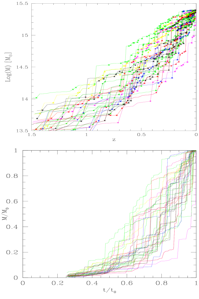
Figure 2: Example of Merger Trees obtained from Monte Carlo simulation in a EdS universe for clusters with present day mass $M_{0}=2.5\times 10^{15}M_{\odot}$: a) $Log(M)-z$; b) $M/M_{0}-t/t_{0}$ with t cosmic time; $t_{0}$ present time.

4 Ram Pressure Stripping, turbulence and MHD waves

4.1 Turbulence injection rate

The passage of the infalling subhalos through the main cluster during mergers induce large–scale bulk flows with velocities of the order of $\sim 1000$ km s^-1 or larger. Numerical simulations of merging clusters (e.g., Roettiger, Loken, Burns 1997; Ricker & Sarazin 2001; Tormen et al. 2004) provide a detailed description of the gasdynamics during a merger event. It has been found that subclusters generate laminar bulk flows through the sweeped volume of the main clusters which inject eddies via Kelvin–Helmholtz instabilities at the interface of the bulk flows and the primary cluster gas. Finally these eddies redistribute the energy of the merger through the cluster volume in a few Gyrs by injecting random and turbulent velocity fields.

The impact velocity between the subclusters increases at the beginning of the merger and then it saturates when the subclusters interpenetrate each other. Depending on the initial conditions and on the mass ratio of the two subclusters, during the merging process the infalling halos may be efficiently stripped due to the ram–pressure. However, the numerical simulations show that the efficiency of the ram pressure stripping is reduced by the formation of a bow shock on the leading age of the subcluster. This bow shock forms an oblique boundary layer which slows the gas flow and redirect it around the core of the subcluster so that, at least in the case of mergers with mass ratios $<10$, a significant amount of the subcluster gas is found to be still self–bounded after the first passage through the central regions of the main cluster (Roettiger et al. 1997; Tormen et al. 2004).

Due to the complicated physics involved in these events, the details of the injection and evolution of turbulent motions in galaxy clusters during merging processes are essentially a still unexplored issue. However, turbulence should be basically driven by the $PdV$ work done by the infalling halos through the volume of the primary cluster and the turbulent motions should be initially injected within the volume sweeped by the passage of the subhalos (e.g., Fujita, Takizawa, Sarazin 2003). Following this simple scenario, in this Section we estimate the rate of turbulence injected during a merger event. As a necessary approximation (due to the PS formalism) in the calculations, we assume that subclusters undergo only central collisions.

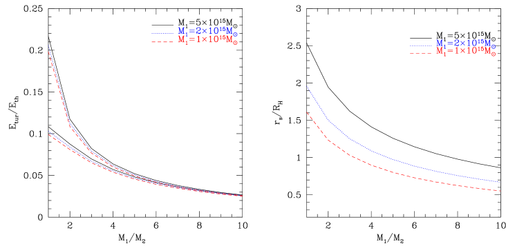
Figure 3: Panel a): Ratio between the energy injected in form of turbulence and the thermal energy of the system as a function of the mass ratio of the two subclusters. Thermal energy is calculated for both the sum of the two subclusters (lower lines) and for the main cluster alone (upper lines). We stress that in the case of a mass ratio $\leq 1.5$ our approach is quite inadequate because essentially no primary cluster exists, however these mergers are very rare events and do not dominate the injection of turbulence in our model. Panel b): Ratio between the stripping radius and the radius of the radio halos (assuming $R_{H}=500h_{50}^{-1}$ kpc) reported as a function of the mass ratio of the two subclusters. In both panels calculations are obtained following the recipes given in Sect. 4.1 for a $M=5$, (solid lines), 2 (dotted lines), and $1\times 10^{15}M_{\odot}$ (dashed lines) clusters.

The relative impact velocity of two subclusters with mass $M_{max}$ and $M_{min}$ which collide (at a distance $R_{max}$ between the centers) starting from an initial distance $d_{o}$ with zero velocity is given by (e.g., Sarazin 2002):

$$v_{i}\simeq\Bigg{(}2G\frac{(M_{max}+M_{min})}{R_{max}}\bigg{(}1-\frac{1}{\eta_{v}}\bigg{)}\Bigg{)}^{1/2}$$ (9)

where $d_{o}=\eta_{v}R_{max}$, $\eta_{v}\simeq 4\big{(}\frac{M_{max}+M_{min}}{M_{max}}\big{)}^{1/3}$, and $R_{max}$ is the virial radius of the main cluster, i.e. :

$$R_{max}=\Bigg{[}\frac{3M_{max}}{4\pi\Delta_{c}(z)\rho_{crit}(z)}\Bigg{]}^{1/3}$$ (10)

$\rho_{crit}(z)$ is the critical density at redshift z and $\Delta_{c}(z)=18\pi^{2}\simeq 180$ is the ratio of the average density of the cluster to the critical density at redshift z.

While the smaller subcluster crosses the larger one, it is stripped due to the effect of the ram–pressure. The stripping is efficient outside a radius $r_{s}$ (stripping radius) at which equipartition between static and ram–pressure is established, i.e. :

$$\overline{\rho}_{max}v_{i}^{2}=\frac{\rho_{min}(r_{s})K_{B}T_{min}}{\mu m_{p}}$$ (11)

where, as an approximation, $\overline{\rho}_{max}$ is fixed at the average density of the ICM of the larger subcluster :

$$\overline{\rho}_{max}=\bigg{(}\frac{M_{max}}{\frac{4}{3}\pi R_{max}^{3}}\bigg{)}\times f_{b}\,,$$ (12)

with $f_{b}=0.25\,(\frac{h}{0.5})^{-3/2}$ the observed barion fraction of clusters (Ettori & Fabian 1999, Arnaud & Evrard 1999). Eq.(11) is solved numerically at each merger event assuming that the density profile of the ICM of the smaller cluster, $\rho_{min}$, is described by a $\beta$-model (Cavaliere & Fusco-Femiano, 1976):

$$\rho_{min}(r)=\rho_{min}(0)\bigg{[}1+(\frac{r}{r_{c}})^{2}\bigg{]}^{-3\beta_{\rm x}/2}$$ (13)

where the normalization is given by :

$$\rho_{min}(0)={{f_{b}M_{min}}\over{4\pi}}\Bigg{\{}\int_{0}^{R_{v}^{M_{min}}}drr^{2}\bigg{[}1+(\frac{r}{r_{c}})^{2}\bigg{]}^{-3\beta_{\rm x}/2}\Bigg{\}}^{-1}$$ (14)

where a core radius $r_{c}=0.1\,\,R_{min}$ and $\beta_{\rm x}\simeq 0.8$ are assumed. The temperature of the smaller cluster, $T_{min}$, in Eq.(11) is estimated making use of the observed M-T relationship (e.g., Nevalainen et al. 2000). As a general remark we stress that the value of the stripping radius obtained above would give the mean value of $r_{s}$ during a merger and it is not the minimum $r_{s}$. In qualitatively agreement with numerical simulations, this approach yields $r_{s}\rightarrow 0$ in the case of mergers with large mass ratios between the two colliding subclusters.

The motion of the smaller cluster through the ICM of the main one generates fluid turbulence. Following Fujita et al.(2003) we assume that turbulence is initially injected in the sweeped volume, $V_{t}\sim\pi r_{s}^{2}R_{max}$, with a maximum turbulence lenght scale of the order of $2\times r_{s}$. The total energy injected in turbulence during a merger event is thus $E_{t}\simeq\overline{\rho}_{max,s}\,v_{i}^{2}V_{t}$, where $\overline{\rho}_{max,s}$ is the ICM density of the main cluster averaged on the sweeped cylinder. We assume that the duration of the injection is of the order of a crossing time, $\tau_{cros}\simeq R_{max}/v_{i}$, then the turbulence is dissipated in a relatively short time.

The use of the averaged density of the ICM of the primary cluster, $\overline{\rho}_{max}$, of the initial impact velocity between the subclusters, $v_{i}$, and of the density of the main cluster averaged on the sweeped cylinder, $\overline{\rho}_{max,s}$ in the caluclations of the injected turbulence is a necessary simplification which however guarantees a basic estimate of the averaged injected turbulence in the ICM and which does not depend on essentially unknown details. For seek of completeness, in Fig. 3a we report the typical ratio between turbulent energy injected by a merger event and the thermal energy of the system as a function of the mass ratio between the two colliding subclusters; it is found that major mergers may channel about 10-15 % of the thermal energy in the form of large scale turbulence. In Fig. 3b we also report the value of the stripping radius as a function of the mass ratio of the two colliding subclusters. It is found that $r_{s}$ (i.e., the mean value of $r_{s}$ during a merger event) is typically larger than the radius of the radio halos, $R_{H}$, for the merger events which mainly contribute to the injection of cluster turbulence in our model. If the sweeped volume is smaller than that of the radio halo, we assume that the injected turbulence is diffused over the volume of the radio halo, $V_{H}=\frac{4}{3}\pi R_{H}^{3}$, which is basically equivalent to assume that the integral cross section of the ensemble of minor mergers which occur in a time interval of $\sim$Gyr is comparable to $R_{H}$.

Under these hypothesis, the injection rate per unit volume of turbulence is given by :

$$\frac{E_{t}}{\tau_{cros}\times V_{H}}\simeq\frac{\overline{\rho}_{max,s}}{R_{max}}v_{i}^{3}\bigg{(}\frac{V_{t}}{V_{H}}\bigg{)}$$ (15)

Figure 4: Evolution of the thermal energy (solid lines) and of the energy injected in fluid turbulence (dashed lines) integrated during cluster life (at redshift $z$) in typical galaxy clusters. The thin lines are for a cluster with present time $M_{0}=10^{15}M_{\odot}$ and the thick lines are for a cluster with present time $M_{0}=5\times 10^{14}M_{\odot}$.

As a relevant example, in Fig.(4) we report the cosmological evolution of the thermal energy of galaxy clusters with different masses, together with the total energy injected in form of turbulence in the ICM. The energy in turbulence is calculated by integrating the contributions from all the merger events. The thermal energy of the considered clusters, calculated assuming the observed M-T relation (e.g., Nevalainen et al. 2000) , increases from about $10^{62}$erg at $z\sim 1$ to a few $10^{64}$erg at the present epoch depending on the mass of the cluster. As it should be, we note that the energy budget injected in turbulence during cluster formation is well below the thermal energy; this indicates the consistency of our calculations. In particular the turbulent energy is found to be $\sim 15\%$ that of the thermal energy in agreement with recent numerical simulations (Sunyaev et al. 2003) and with very recent observational claims (Schuecker et al. 2004). Finally, as reasonably expected, the energy injected in turbulence calculated with our approach is found to roughly scale with the thermal energy of the clusters.

4.2 Spectrum of the magnetosonic waves

Cluster mergers should generate magnetosonic (MS) waves in the ICM, the injected energy and spectrum of these waves depends on many unknown quantities. A reasonable attempt is to assume that a fraction, $\eta_{t}$, of the energy of the turbulence (Sect. 4.1) is in the form of MS waves. We shall consider two extreme scenarios:

• in the first one we assume that MS waves are driven by the plasma instabilities (e.g., Eilek 1979, and ref. therein) which develope in the turbulent field generated during cluster mergers. In this case MS waves may be injected over a broad range of scales. Here, we shall adopt a simple power law injection spectrum of these waves: $I(k)=I_{o}k^{-a}$ for $k>k_{min}\sim\pi/r_{s}$;

• in the second one, we assume that MS waves are basically injected at a single scale, $k=k_{min}\sim\pi/r_{s}$, from which a MHD turbulence cascade is originated.

In both cases the decay time of the MHD turbulence at the maximum/injection scale, $L_{inj}\sim 2r_{s}$, can be estimated as (e.g., Appendix B) $\tau_{kk}(L_{inj})\sim{{r_{s}}\over{\eta_{t}v_{i}}}$, one has :

$$\tau_{kk}({\rm Gyr})\sim 1\times({{v_{i}}\over{2\cdot 10^{3}{\rm km/s}}})^{-1}({{r_{s}}\over{500{\rm kpc}}})({{\eta_{t}}\over{0.25}})^{-1}$$ (16)

which is of the order of a crossing time and thus allows the MHD turbulence to diffuse filling a volume of the order of that of radio halos (or larger) with a fairly uniform intensity.

In the following we focus on the first scenario, while in the Appendix B we consider the second picture. Appendix B demonstrates that these two extreme scenarios lead to very similar results and thus that, in our model, the details of the injection process of the MS waves do not appreciably change the conclusions.

In the case in which a power law spectrum of MS waves is injected in the ICM, one has :

$$\int_{k_{min}}^{k_{max}}I_{o}k^{-a}dk=\eta_{t}\frac{E_{t}}{\tau_{cros}\times V_{H}}$$ (17)

with $k_{min}\sim\pi/r_{s}$ and $k_{max}=\Omega_{p}/v_{M}$ $\Omega_{p}$ being the proton cyclotron frequency and $v_{M}$ the magnetosonic velocity (Eq. 40). From Eq. (17) we find:

$$I_{o}=\left\{\begin{array}[]{ll}\frac{E_{MS}}{\tau_{cros}}\times\frac{(a-1)}{V_{H}}k_{min}^{-(1-a)}&(r_{s}\leq R_{H})\\ &\\ \frac{E_{MS}}{\tau_{cros}}\times\frac{(a-1)}{V_{H}}k_{min}^{-(1-a)}\times(\frac{R_{H}}{r_{s}})^{2}&(r_{s}>R_{H})\\ \end{array}\right.$$ (21)

Thus, the injection of the MS waves is obtained by combining Eqs.(15) and (21). $\eta_{t}$ is the first free parameter of our model, in order to have a self–consistent modelling it should be $\eta_{t}<1$.

In general, the spectrum of MHD waves injected in the ICM evolves due to wave–wave and wave–particle coupling. The combination of these processes produces a modified spectrum of the waves, $W_{\rm k}(t)$. In the quasi linear regime the spectrum of the waves can be calculated solving a continuity equation in the wavenumber space:

$${{\partial W_{\rm k}(t)}\over{\partial t}}={{\partial}\over{\partial k}}\left(D_{\rm kk}{{\partial W_{\rm k}(t)}\over{\partial k}}\right)-\sum_{i=1}^{n}\Gamma^{\rm i}(k)W_{\rm k}(t)$$

$$+I_{\rm k}(t)$$ (22)

The first term on the right hand describes the wave–wave interaction, with diffusion coefficient $D_{\rm kk}=k^{2}/\tau_{s}$ (with $\tau_{s}$ the spectral energy transfer time). The second term in Eq.(22) describes the damping with the relativistic and thermal particles in the ICM, and the damping due to thermal viscosity. In the following, we shall neglect the term due to the wave–wave interaction, this is justified provided that the time–scale of the dampings are smaller than that of the wave–wave cascade (or comparable), at least for the range of scales which contribute to the acceleration process (assuming spectra flatter than $W_{k}\propto k^{-2}$; see also Appendix B). Under physical conditions typical of the ICM the most important damping in the collisionless regime is that with the thermal electrons (e.g., Eilek 1979; see also Sect. 5.2.2). An estimate of this damping rate (for $v_{A}<v_{M}$ as in the ICM) is given by Eilek 1979; a relatively simple formula, consistent whitin a 10% with the Eilek’s results, is:

$$\Gamma_{th,e}=\sqrt{32\pi^{3}}\,n_{th}\,(m_{e}K_{B}T)^{1/2}\big{(}\frac{v_{M}}{B}\big{)}^{2}\frac{{W}_{k}^{B}}{{W}_{k}}\,{\cal I}(x)\,k$$ (23)

where $n_{th}$ is the number density of the thermal electrons, ${W}^{B}_{k}$ is the turbulent magnetic energy density, ${W}^{B}_{k}={W}_{k}\times(1+8\pi P/B^{2})^{-1}$, with $P\simeq 2n_{th}K_{B}T$ the thermal pressure, $B$ the plasma magnetic field (e.g., Barnes & Scargle 1973) and ${\cal I}(x)$ is a numerical value given by :

$${\cal I}(x)=2\,\int_{1}^{+\infty}dx\,\Big{(}\frac{1}{x}-\frac{1}{x^{3}}\Big{)}\,e^{-[x^{2}(\frac{v_{M}}{v_{th}})^{2}]}$$ (24)

where $x=\frac{p_{\|}}{m_{e}v_{M}}$, with $p_{\|}$ the component of the momentum of the thermal electrons along the magnetic field lines and $v_{th}=(2\,K_{B}\,T/m_{e})^{1/2}$.

Since for each merger event we are interested in the evolution of the spectrum of the injected waves on a time scale of $\sim 1$ Gyr, which is orders of magnitude longer than the typical time scales of the damping processes, the spectrum of the waves is expected to approach a stationary solution ($\partial W_{\rm k}/\partial t=0$). From Eq. (22) this solution is given by :

$$W_{\rm k}\simeq\frac{I(\rm k)}{\Gamma_{\rm th,e}(k)}=\frac{I(\rm k)}{f(T)\,k}$$ (25)

In Sect. 5.2 we will derive the efficiency of electron acceleration due to the MS waves. Here we would just point out that the acceleration time, $\tau_{\rm acc}$, depends on :

$$\tau_{\rm acc}^{-1}\propto\int_{k_{min}}^{k_{max}}kW_{\rm k}dk$$ (26)

which leads (making use of Eqs. 21 and 25) to the nice result that the acceleration time in our model, and under our assumptions, does not depend on the slope of the injection spectrum of MS waves (which depends on basically–unknown details of the injection mechanism) and on the value of $k_{min}$.

4.3 Spectrum of MS waves during cluster formation

In this Section we estimate the spectrum of MS waves resulting from the combination of the contributions of several mergers during the process of cluster formation. For a given galaxy cluster, we define $z_{i}^{j}$ to be the redshift at which the $j^{th}$ merger event starts. For an Einstein-De Sitter model, the corresponding time, $t_{i}^{j}$, is :

$$t_{i}^{j}=\frac{2}{3H_{o}}\frac{1}{(1+z_{i}^{j})^{3/2}}$$ (27)

In our simple modelling we assume that the duration time of a merger is of the order of a crossing time, $\Delta t=t_{cros}^{j}$, and that turbulence is injected during this time interval and then suddenly dissipated via damping processes . Thus the turbulence injected during the $j^{th}$ merger is dissipated at time $t_{f}^{j}=t_{i}^{j}+t_{cross}^{j}$ and the corresponding redshift is given by :

$$z_{f}^{j}=(\frac{2}{3H_{o}t_{f}^{j}})^{2/3}-1$$ (28)

We describe the spectrum of the MS–waves established during the $j^{th}$ merger event as :

$$W_{k}^{j}(z)=W_{k}^{j}(z_{i}^{j})\times S^{j}(z)$$ (29)

were $S^{j}(z)$ is a step function defined as :

$$S^{j}(z)=\left\{\begin{array}[]{ll}1&(z_{f}^{j}<z<z_{i}^{j})\\ &\\ 0&({\rm otherwise})\\ \end{array}\right.$$ (33)

According to the hierarchical scenario adopted in this paper, clusters undergo several merger events which contribute to the injection of turbulence yielding a combined spectrum of MS–waves. Since under stationary conditions and neglecting the wave–wave interaction term, Eq.(22) is a linear differential equation, the spectrum of the MS–waves resulting from the combination of the different merger events is given by the sum of all the contributions (Eq.29), i.e. :

$${\cal W}_{\rm k}(z)=\sum_{j}W_{k}^{j}(z_{i}^{j})\times S^{j}(z)$$ (34)

5 Particle Evolution and Acceleration

Völk et al. (1996) and Berezinsky et al. (1997) have shown that cosmic ray protons are most likely accumulated in galaxy clusters as their diffusion time scale is of the order or larger than the Hubble time. An even stronger conclusion can be applied to the case of the relativistic electrons injected in the ICM. Indeed, by assuming a Kolmogorov spectrum for the turbulent field the parallel diffusion length, $L_{D}$, of relativistic electrons is given by (e.g., Brunetti 2003):

$$L_{D}\simeq 120\,\left({{\gamma/10^{2}}\over{B_{\mu G}}}\right)^{{{1}\over{6}}}\left({{l_{o}}\over{100\,{\rm kpc}}}\right)^{{{3}\over{4}}}{{\tau_{D}}\over{{\rm Gyr}}}\,\,\,({\rm kpc})$$ (35)

where $l_{o}$ is the maximum coherence scale of the magnetic field fluctuations. We notice that $\gamma\sim 100-300$ relic relativistic electrons cannot diffuse more than 200 kpc during their life–time (a few Gyrs, e.g., Sarazin 1999). When turbulence is generated in galaxy clusters the ensuing increase of the particle-wave scattering frequency would further reduce the net diffusion coefficient. Only in the case of very strong turbulence anomalous particle turbulent diffusion may allow electrons to diffuse over larger scales (e.g., Duffy 1994; Enßlin 2003), but the requested conditions are well beyond those assumed in the present paper.

Thus, we can safely assume that electrons injected by some mechanism in the ICM simply follow the thermal plasma and magnetic field. Under this condition, the time evolution of relativistic electrons with isotropic momentum distribution is provided by a Fokker-Planck equation (e.g., Tsytovich 1966; Borovsky & Eilek 1986) for the electron number density :

$${{\partial N(p,t)}\over{\partial t}}={{\partial}\over{\partial p}}\left[N(p,t)\left({\big{|}{{dp}\over{dt}}\big{|}}_{\rm rad}+{\big{|}{{dp}\over{dt}}\big{|}}_{\rm c}-{2\over{p}}D_{\rm pp}\right)\right]+$$

$${{\partial}\over{\partial p}}\left[D_{\rm pp}{{\partial N(p,t)}\over{\partial p}}\right]+Q_{e}(p,t)$$ (36)

where $D_{\rm pp}$ is the electron diffusion coefficient in the momentum space due to the interaction with the MS waves, ${dp/dt}_{\rm i}$ and ${dp/dt}_{\rm rad}$ are the terms due to ionization and radiative losses and $Q_{e}$ is an isotropic electron source term.

5.1 Particle injection

A relevant contribution to the injection of cosmic rays in clusters of galaxies comes from Active Galactic Nuclei (AGN). AGNs indeed inject in the ICM a considerable amount of energy in relativistic particles and also in magnetic fields, likely extracted from the accretion power of their central black hole (Enßlin et al., 1997).

Powerful Galactic Winds (GW) can inject relativistic particles and magnetic fields in the ICM (Völk & Atoyan 1999). Although the present day level of starburst activity is low and thus this mechanism is not expected to produce a significant contribution, it is expected that these winds were more powerful during early starburst activity. Some evidence that powerful GW were more frequent in the past comes from the observed iron abundance in galaxy clusters (Völk et al. 1996).

In addition, cluster formation is also believed to provide a possible contribution to the injection of cosmic rays in the ICM due to the formation of shocks which may accelerate relativistic particles (Blasi 2001; Takizawa & Naito, 2000; Miniati et al., 2001; Fujita & Sarazin 2001). The efficiency of this mechanism is related to the Mach number of these shocks which is an issue still under debate. Semi–analytical calculations based on PS-Monte Carlo techniques (Gabici & Blasi 2003; Berrington & Dermer 2003) find that the bulk of the shocks have Mach numbers of order 1.5, as also observed by Chandra (e.g., Markevitch et al. 2003). First cosmological numerical simulations found that the Mach number of merger and internal flow shocks peacks at ${\cal M}\sim 5$ (Miniati et al. 2000), and that the bulk of the energy is dissipated at $4\leq{\cal M}\leq 10$ shocks (Miniati 2002). On the other hand, more recent numerical simulations find more weak shocks with the bulk of the energy dissipation (thermal energy and cosmic rays) at internal shocks with $2\leq{\cal M}\leq 4$ (Ryu et al., 2003). However, the comparison with semi-analytical calculations appears difficult because of a different classification of the shocks in the two approaches.

Independently from the specific scenario adopted for the injection of relativistic particles, a power law spectrum for the injection rate of relativistic electrons up to a maximum momentum, $p_{\rm max}$, can be reasonably assumed :

$$Q_{\rm e}(p,t)=K_{\rm e}(t)p^{-s}$$ (37)

We parameterize the injection rate by assuming that the total energy injected in cosmic ray electrons (for $p>p_{\rm min}$) during the cluster life is a fraction, $\eta_{e}$, of the total thermal energy of the cluster at $z=0$, i.e. :

$$\eta_{e}={{c}\over{{\cal E}_{\rm th}}}\int_{t=t(z)}^{t=t(0)}d\tau\int_{p_{\rm min}}^{p_{\rm max}}Q_{e}(p,\tau)\,p\,dp$$ (38)

where ${\cal E}_{\rm th}$ is the present day thermal energy density of the ICM.

The injection rate should depend on the number and energetics of AGNs and GWs in galaxy clusters which are expected to be considerably larger at high redshifts. However, since electrons injected at relatively high redshifts cool very rapidly because of the combination of high energy losses and low efficiency of the particle acceleration mechsnism (Fig. 5), only the electrons injected at relatively low redshifts can be accelerated and therefore contribute to the non-thermal emission observed at $z<0.2$. As a simplification, we adopt a constant injection rate of electrons so that (for $s>2$) the normalization of the spectrum of the injection rate is given by :

$$K_{\rm e}\sim{{s-2}\over{c}}\eta_{e}{\cal E}_{\rm th}p_{\rm min}^{s-2}\tau_{H}^{-1}$$ (39)

where $\tau_{H}$ is the Hubble time. $\eta_{e}$ is the second free parameter in our model. In the following we use $s=2.5$, $p_{\rm min}/mc=60$, and $p_{\rm max}/mc=10^{4}$; as discussed in Sect. 8 the basic results of our model do not depend on the values adopted for these parameters.

5.2 Energy gains and losses of the relativistic particles

Fast MS waves can accelerate relativistic particles via particle–wave interaction. This interaction occurs with both thermal (expecially) and relativistic particles via Landau damping, the strongest damping of MS waves in the collisionless regime. The necessary condition (Melrose 1968; Eilek 1979) is $\omega-k_{\|}v_{\|}=0$, where $\omega$ is the frequency of the wave, $k_{\|}$ is the wavenumber projected along the magnetic field, and $v_{\|}=v\mu$ is the projected-particle velocity. Under the typical conditions of the ICM, the dispersion relation for MS waves in an isotropic plasma is given by (e.g., Eilek 1979):

$$\frac{\omega^{2}}{k^{2}}=v_{M}^{2}\simeq\frac{4}{3}v_{ion}^{2}+v_{A}^{2}$$ (40)

where $v_{ion}$ and $v_{A}$ are the ion-sound velocity and the Alfvén velocity, respectively. In a isotropic distribution of waves and particle momenta the diffusion coefficient in the momentum space, for $v_{A}<v_{M}$, is given by Eilek (1979). This can be expressed as:

$$D_{\rm pp}(p,t)\simeq 4.45\,\pi^{2}\,{{v_{M}^{2}}\over{c}}{{p^{2}}\over{B^{2}}}\int_{k_{min}}^{k_{max}}k{\cal W}^{B}_{k}(t)dk$$ (41)

The acceleration time scale, which in this case does not depend of the particle energy, is given by :

$$\tau_{\rm acc}^{-1}=\chi\simeq 2{{D_{\rm pp}}\over{p^{2}}}$$ (42)

and thus the systematic energy gain of particles interacting with MS waves is given by :

$$\left({{dp}\over{dt}}\right)_{\rm acc}^{sys}=\chi\,p$$ (43)

5.2.1 Electrons

Relativistic electrons with momentum $p_{\rm e}=m_{\rm e}c\gamma$ in the ICM lose energy through ionization losses and Coulomb collisions (Sarazin 1999):

$$\left({{dp}\over{dt}}\right)_{\rm c}=\,-3.3\times 10^{-29}n_{\rm th}\left[1+{{{\ln}(\gamma/{n_{\rm th}})}\over{75}}\right]$$ (44)

where $n_{\rm th}$ is the number density of the thermal plasma.

Relativistic electrons also lose energy via synchrotron emission and inverse Compton scattering off the CMB photons:

$$\left({{dp}\over{dt}}\right)_{\rm rad}=\,-4.8\times 10^{-4}p^{2}\left[\left({{B_{\mu G}}\over{3.2}}\right)^{2}{{\sin^{2}\theta}\over{2/3}}+(1+z)^{4}\right]$$ (45)

$${}\,\,\,\,\,\,\,\,\,\,\,\,\,\,\,\,\,\ =-\frac{\beta p^{2}}{m_{e}\,c}$$

where $B_{\mu G}$ is the magnetic field strength in $\mu G$ and $\theta$ is the pitch angle of the emitting electrons; in case of efficient isotropization of the electron momenta it is possible to average over all possible pitch angles, so that $<\sin^{2}\theta>=2/3$.

Eqs.(41), (44) and (45) gives the coefficient of the Fokker-Plank equation (36).

5.2.2 Protons

For seek of completeness in this Section we briefly discuss the case of relativistic protons.

The main channel of energy losses for these particles is represented by inelastic proton-proton collisions, which is a threshold reaction that requires protons with kinetic energy larger than $\sim 300$ MeV. The time scale of this process is $\tau_{pp}\sim 30(n_{\rm th}/10^{-3})^{-1}$Gyr. The interactions with the ICM may generate an appreciable flux of gamma rays and neutrinos, in addition to a population of secondary electrons (Blasi & Colafrancesco 1999).

Protons which are more energetic than the thermal electrons lose energy due to Coulomb interactions. For trans-relativistic and sub-relativistic protons this channel can easily become the main channel of energy losses in the ICM.

In our calculations we focus on the population of relativistic electrons, do not consider proton acceleration, and neglect the effect of these particles on the efficiency of the electron acceleration.

The resonance condition $v_{M}k=k_{\|}v_{\|}$ implies that only a very small fraction of MS waves (those making an angle $\sim$89–91 degrees with the local B-field) cannot be damped by the thermal electrons, but only by the relativistic particles (protons and electrons), while outside this narrow cone the damping due to the thermal electrons should be the strongest one (e.g., Eilek 1979). As a consequence, since in our calculations we assume a continuous pitch angle isotropization (e.g., Miller et al. 1996) and an isotropic distribution of MS waves which propagate in a complex geometry of the field lines, the damping of MS waves should be dominated by the effect due to the thermal electrons in the ICM.

As an example, we assume that MS waves are injected in the central $\sim$1 Mpc³ of a massive cluster for 0.5–1 Gyr with a total energy budget of the order of that of the thermal ICM within the same region. We calculate particle acceleration and find that about $\sim 4-10\%$ of the energy flux of these waves is channelled into the acceleration of relativistic protons (assuming an initial energy density of these particles of the order of few % of the thermal energy density and $N_{p}(p)\propto p^{-2.2}$): this corresponds to $\leq 1\%$ of the total thermal energy of the cluster. At the same time, we find that only $\sim 0.1\%$ of the energy flux of the MS waves should be channelled into the acceleration of relativistic electrons to produce an HXR luminosity of $\sim 10^{43}$erg s^-1 from the same volume ($\eta_{e}\sim 0.003$, Fig. 6). Consequently the $90-95\%$ of the energy flux of the MS waves is channelled into the thermal electrons and thus the resulting spectrum of these waves may be estimated with good approximation by Eq.(25).

Detailed time dependent calculations which include electron and proton acceleration due to MS waves and a comparison with the case of Alfvén waves will be given in a forthcoming paper (Brunetti et al., in prep.).

6 Radio Halos and HXR tails

6.1 Cluster evolution and electron spectrum

In this Section we combine the formalism developed for the evolution of the turbulence (Sects. 3 & 4) with the recipes for particle acceleration and evolution (Sect. 5) to model the cosmological evolution of the spectrum of the relativistic electrons in galaxy clusters.

The electron–acceleration coefficient, due to the effect of MS waves at redshift $z$, is obtained by combining Eq. (42) with Eqs. (41, 21, 25, 34):

$$\chi(z)\simeq{{2.23\times 10^{-16}\eta_{t}}\over{(R_{H}/500{\rm kpc})^{3}}}\sum_{j}\Bigg{[}\Big{(}{{M_{max}+M_{min}}\over{2\times 10^{15}M_{\odot}}}\,\,{{2.6{\rm Mpc}}\over{R_{max}}}\Big{)}^{3/2}$$ (49)

$${}\times\frac{(r_{s}/500{\rm kpc})^{2}}{(kT/7{\rm keV})^{1/2}}\Bigg{]}_{j}\times\left\{\begin{array}[]{ll}1&{\rm if}\,r_{s}\leq R_{H}\\ &\\ (R_{H}/r_{s})^{2}&{\rm if}\,r_{s}>R_{H}\\ \end{array}\right\}_{j}$$

where only mergers which contribute to the turbulence spectrum at redshift $z$ (Sect. 4.3, Eq.34) are considered. The evolution of the electron spectrum is thus obtained from the numerical solution of the Fokker-Planck equation (Eq. 36) by adopting the values of the coefficient $D_{pp}$ (Eq. 42 and Eq. 49) and of the energy loss terms (Eqs. 44–45) at each redshift.

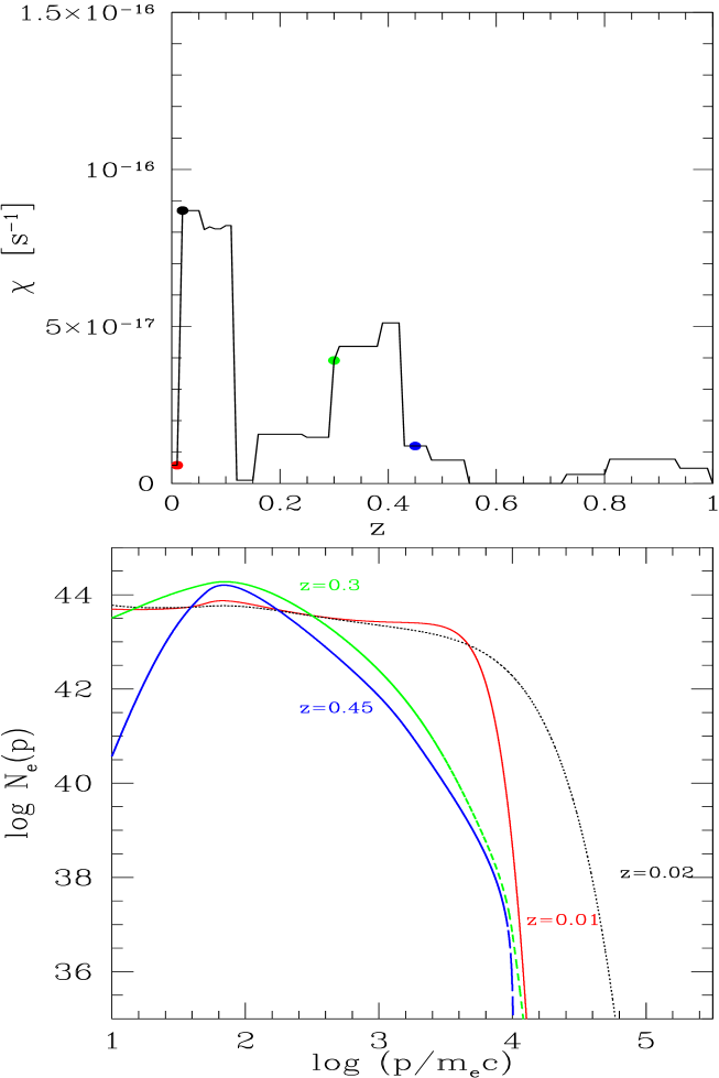
Figure 5: Top panel: evolution with redshift of the electron-acceleration coefficient due to MS waves as obtained from Eq.49 for a cluster of $M_{0}=1\times 10^{15}M_{\odot}$ at the present time. Bottom panel: electrons spectra (in arbitrary units) calculated at different redshifts (also marked in the top panel) for the same cluster. Calculations are performed for $s=2.5$, $B=0.5\mu$G, and $\eta_{t}=0.26$.

In Fig.(5) we report an example of the time evolution of the electron–acceleration coefficient obtained for a typical massive cluster (top panel) and the corresponding spectra of the electrons at different relevant times (bottom panel): an increase of the acceleration coefficient produces an increase of the maximum energy of the electrons. The reported results indicate that cluster–merger activity at low redshift can generate an increse of the cluster turbulence which may be sufficient to accelerate electrons up to $\gamma>>10^{3}$, necessary to produce synchrotron radiation in the radio band. It should be noticed that electrons are accelerated (and cool) with a delay time (of the order of the corresponding electron–acceleration time $\sim\chi^{-1}$) with respect to the abrupt increases (decreases) of the values of the acceleration coefficient.

In Fig.(6) we show the broad band non–thermal emission (synchrotron and IC) from the galaxy cluster reported in Fig. 5 assuming $\eta_{e}=0.003$ and $B=0.5\mu$ G (for the sake of completeness synchrotron and IC equations are given in Appendix C). The aim of this Figure is to show that synchrotron (and IC) luminosities of the order of those of the most luminous radio halos can be reasonably obtained. On the other hand, it should be stressed that the synchrotron spectrum reported in Fig.(6) is obtained assuming a constant value of $B$ through the cluster volume. More reasonable calculations should assume a radial gradient of the magnetic field strength which causes a stretching in frequencies of the synchrotron spectral shape with respect to that of Fig.(6) (e.g., Brunetti et al. 2001; Kuo et al. 2003).

The synchrotron emitted power from radio halos is also expected to increase with increasing the mass of the parent clusters. Indeed the bolometric synchrotron power roughly scales as $P_{\rm syn}\propto B^{2}\gamma_{\rm b}^{2}N_{\rm e}R_{H}^{3}$ where $\gamma_{b}=\frac{\chi}{\beta}$ is the maximum energy of the accelerated electrons ($\beta$ is the total energy–loss coefficient, Eq. 45) and $N_{\rm e}$ is the number of relativistic electrons in the cluster emitting volume. During major mergers, from Eq.(49, with $T\propto M^{a}$, $a\sim 0.55-0.67$) one has :

$$P_{\rm syn}\propto N_{\rm e}M^{2-a}g(r_{s},R_{H})^{2}{{B^{2}}\over{(B^{2}+B_{\rm cmb}^{2})^{2}}}$$ (50)

where $g(rs,R_{H})$ ($g=r_{s}^{2}$ for $r_{s}\leq R_{H}$ and $g=R_{H}^{2}$ for $r_{s}>R_{H}$) is a slightly increasing function of cluster mass. Thus assuming $B<3\mu$G one can find that the synchrotron power would roughly scale as $P_{\rm syn}\propto M^{b(M)}<N_{\rm e}B^{2}>_{(M)}$, where $b(M)\sim 1.5-2.5$ ($b=1.5$ for $M\geq 3\cdot 10^{15}M_{\odot}$ and $b=2.5$ for $M<10^{15}M_{\odot}$), and $<N_{\rm e}B^{2}>_{(M)}$ is expected to increase with cluster mass. Although studies of the synchrotron power – mass (or temperature) correlation for radio halos use the monochromatic synchrotron emission at 1.4 GHz (e.g., Liang et al. 2000; Govoni et al. 2001; Giovannini & Feretti 2002), the above expectations seem to be in line with observations.

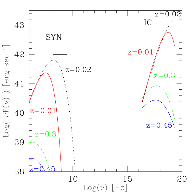
Figure 6: Broad band synchrotron (SYN) and Inverse Compton (IC) spectra calculated for the case reported in Fig.5 and for $\eta_{e}=0.003$, $R_{H}=500$ kpc, and $B=0.5\mu$G. Horizontal bars give the radio (used for radio halos) and HXR observational range of frequencies.

6.2 On the required values of $\eta_{t}$ and $\eta_{e}$

In this Section we derive the range of values of the two free parameters of our model, $\eta_{t}$ and $\eta_{e}$, which provide a reasonable agreement with the general properties of radio halos. In order to check the reliability of the obtained values, these are then compared with independent findings and general expectations from both analytical and numerical calculations.

The first free parameter is $\eta_{t}$ which is defined as the fraction of the fluid turbulence in MS waves. The value of $\eta_{t}$ drives the efficiency of the electron acceleration and thus the resulting maximum energy of electrons, $\gamma_{b}=\frac{\chi}{\beta}$, ($\beta$ is the total energy–loss coefficient, Eq. 45), and the maximum synchrotron emitted frequency $\nu_{b}=\frac{3}{4\pi}\frac{eB}{m_{e}c}\gamma_{b}^{2}$. Under the assumption that the losses of the electrons are dominated by the IC mechanism, the acceleration coefficient is thus related to the break frequency by :

$$\chi\simeq 6.3\times 10^{-21}\nu_{b}^{1/2}B_{\mu G}^{-1/2}(1+z)^{4}$$ (51)

The values of $\eta_{t}$ are constrained by requiring that the accelerated electrons can produce synchrotron radiation in the radio band with the spectral shape observed in the case of radio halos, i.e. with spectral index $\alpha=1.1-1.5$ between 327 and 1400 MHz (e.g., Kempner & Sarazin 2001). The synchrotron spectral index between two fixed frequencies depends on the value of $\nu_{b}$ and also on the shape of the spectrum of the emitting electrons. Given the typical shape of the spectrum of the emitting electrons accelerated during cluster mergers in our calculations, we are able to estimate the minimum typical value of $\nu_{b}$ necessary to account for the spectral indices of the observed radio halos: $\nu_{b}>70$ MHz is obtained. From Eq. (51), this limit translates into a limit on $\chi$ (given in Eq.49) :

$$\chi(\eta_{t})\,\,$\raise 2.0pt\hbox{$>$} \kern-11.00008pt\lower 4.0pt\hbox{$\sim$}$\,\,\chi_{min}=7.4\times 10^{-17}(1+z)^{4}\bigg{(}\frac{B_{\mu G}}{0.5}\bigg{)}^{-1/2}s^{-1}$$ (52)

Radio halos have a typical size $R_{H}\sim$500 Kpc and they are found in massive galaxy clusters (M$>$ $\sim$$10^{15}M_{\odot}$). Thus we derive the value of $\chi$ for these typical clusters in our synthetic population and find that $\eta_{t}=0.2-0.3$ is required to satisfy the condition of Eq. (52) during major mergers (at $z<0.2$; $B\sim 0.5\mu$G is adopted). This is the first important result of our modelling since it basically proves that if a fraction of the kinetic energy of cluster mergers is channelled into MS waves then this is sufficient to power particle acceleration in the ICM with the efficiency requested in the case of radio halos. Although there are no numerical studies which are aimed at a detailed investigation of the cluster turbulence injected during merging processes, a general finding of high resolution numerical simulations is that a relevant fraction (10-30 %) of the thermal energy in galaxy clusters is in the form of compressible plasma turbulence (e.g., Sunyaev et al. 2003 and ref. therein). This is in line with the requirements of our model.

The second free parameter in our model is $\eta_{e}$ which gives the ratio between the energy injected in relativistic electrons during the cluster life and the present day thermal energy of the ICM. The values of $\eta_{e}$ can be constrained by requiring that the model reproduces the typical radio ($L_{R}$) and hard-X ray ($L_{HX}$) luminosities observed in galaxy clusters: $L_{R}=10^{40}-10^{41}$erg$s^{-1}$ (Feretti 2003) and $L_{HX}=10^{43}-10^{44}$erg$s^{-1}$ (Fusco-Femiano et al.2003). We derive the requested values for typical massive galaxy clusters in our synthetic population during the time intervals in which the condition of Eq. (52) is satisfied. Making use of Eqs. (39), (72), and  (74) we find that $\eta_{e}=10^{-4}-10^{-3}$ is sufficient to match the observed luminosities at $z<0.2$ ($B\sim 0.5\mu$G is assumed). The above $\eta_{e}$–values are very reasonable for massive clusters (e.g., Sect.5) and they are also much smaller than those assumed in other modellings of non–thermal emission from galaxy clusters (e.g., $\eta_{e}\simeq 0.1$, Sarazin 1999). This is mainly because in our model the resulting spectrum of the emitting electrons during an efficient acceleration period is not a simple power law, but it is peaked at the energies required to emit the synchrotron and IC radiation (e.g., Fig. 6) and this strongly increases the emitting efficiency (see also Sect. 8).

7 Statistics and Comparison with Observations

In Sect. 6.2 we have derived a criterion for radio halo formation: clusters may have radio halos if $\chi(\eta_{t})\geq\chi_{min}$. By making use of this criterion, the goal of this Section is to calculate the formation probability of radio halos with cluster mass and to compare expectations with observational constraints.

In order to have a prompt comparison with observations we calculate the formation probability in the redshift bin $z$=0–0.2 for three mass bins of the parent clusters $\Delta M$: $<9\times 10^{14}M_{\odot}$, $9\times 10^{14}<M<1.8\times 10^{15}M_{\odot}$, and $1.8\times 10^{15}<M<3.6\times 10^{15}M_{\odot}$, which are consistent with the luminosity bins adopted to draw the observed statistics (Giovannini et al. 1999; Giovannini & Feretti 2002).

First we run a large number, ${\cal{N}}$, of trees for different cluster masses at $z=0$, ranging from $\sim 10^{14}M_{\odot}$ to $\sim 10^{16}M_{\odot}$. Thus, for each $M$, we estimate the formation probability of radio halos in the mass bin $\Delta M$ as :

$$f_{M}^{\Delta M}=\frac{\sum_{j=1}^{{\cal{N}}}t_{u}^{j}}{\sum_{j=1}^{{{\cal{N}}}}(t_{u}^{j}+t_{d}^{j})}$$ (53)

where $t_{u}$ is the time that the cluster spends at $z<0.2$ in the mass bin $\Delta M$ with $\chi\geq\chi_{min}$ and $t_{d}$ is the time that the same cluster spends in $\Delta M$ with $\chi<\chi_{min}$.

Thus the total probability of halo formation in the mass bin $\Delta M$ is obtained by combining all the contributions (Eq. 53) weighted with the present day mass function of clusters.

We consider two possible cluster mass functions: the Press & Schecther mass function (1974, P&S):

$$n_{\rm PS}(M,z)\,dM=\sqrt{\frac{2}{\pi}}\,\frac{\overline{\rho}}{M}\,\frac{\delta_{c}(z)}{\sigma^{2}(M)}\,\left|\frac{d\,\sigma(M)}{d\,M}\right|\times$$

$$\exp\left[-\frac{\delta_{c}^{2}(z)}{2\sigma^{2}(M)}\right]\,dM\,,$$ (54)

were $\sigma^{2}(M)$ is given by Eq.(5) and the other quantities are given in Sect. 3.1, and the Sheth & Tormen (1999, S&T) mass function which is obtained from a fit to numerical simulations and which predicts smaller and larger values of the cluster number density for small and large masses, respectively. We checked that the probability to have a radio halo obtained by making use of the P&S and S&T mass functions are consistent within few percent for the considered mass bins.

In Fig. 7 we plot the occurrence of radio halos with a typical radius $R_{H}\sim 500$ kpc, as a function of $\eta_{t}$ compared with the observated statistics (see caption). We find that the relatively high occurence of radio halos observed in massive clusters can be well reproduced by our modelling under very reasonable conditions, i.e. that a fraction of 20-30% of the energy of the turbulent motions (about few percent of the thermal energy) is in the form of compressible MS waves. In addition, we find that there is a range of values of the parameter $\eta_{t}$ ($0.2\leq\eta_{t}\leq 0.26$, for $B\sim 0.5\mu$G) for which the theoretical expectations are in agreement with the observed statistics in both the considered mass bins: $\sim 30\%$ and $\sim 4\%$ in the high and medium mass bins considered, respectively. Finally, we find that the expected probability to form giant radio halos in smaller clusters (not reported in Fig. 7) is negligible, in agreement with the observations.

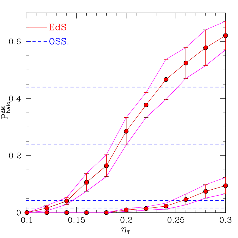
Figure 7: Expected formation probability of radio halos ($R_{H}\simeq 500$ kpc, $B\sim 0.5\mu$G) in a EdS cosmology as a function of parameter $\eta_{t}$ in two different mass bins (solid lines with error bars): binA$=[1.8-3.6]\,10^{15}M_{\odot}$ and binB$=[0.9-1.8]\,10^{15}M_{\odot}$. The two bottom dashed lines mark the observed probabilities for radio halos in the mass binB while the two top dashed lines mark the observed probabilities in the mass binA. The two reported observational ranges account for 1$\sigma$ errors. The theoretical errors are estimated by extracting sub-samples of galaxy clusters from the synthetic population with a Monte Carlo procedure.

8 Summary and Discussion

Crucial constraints on the origin of radio halos are provided by statistical studies which show a connection between the formation of these sources and cluster mergers, and also find an abrupt increase of the occurence of radio halos with the mass of the parent clusters.

- The first goal of the present paper is to check if cluster turbulence generated during mergers may be able to drive efficient particle acceleration processes in the ICM.

- The second goal, in the framework of the turbulent–acceleration hypothesis, is to investigate if the hierarchical formation process of galaxy clusters can naturally account for the increase of the radio halos’ occurrence with cluster mass.

To achieve these goals we developed a statistical magneto–turbulent model which is based on the following steps :

• Extensive merger trees of galaxy clusters with different present day masses are obtained. The trees are calculated making use of a procedure of Binary Merger Tree Method which is based on the extended PS formalism (Sect. 3). The temperature of the ICM is estimated at each redshift from the observed M–T relationships.

• Cluster turbulence is assumed to be injected during cluster mergers by the crossing of the infalling subclusters into the larger ones. To be conservative, turbulence is assumed to be injected in the major subcluster only within the volume sweeped by the minor subcluster (Sect. 4). The injection rate of MS waves is assumed to be a fraction, ${\bf\eta_{t}}$, of the turbulence injection rate.

  The injection spectrum of MS waves is assumed to be a simple power law which extends over a broad range of scales (Sect. 4), or a delta–function from which turbulent cascade is originated (Appendix B). In both cases the maximum/injection scale is fixed at $L_{inj}\sim 2r_{s}$. The resulting spectrum of MS waves is then calculated assuming stationary conditions within a crossing time for each merger and by taking into account the relevant damping processes (or cascading processes) in the ICM (Sect. 4). The evolution of the spectrum of MS waves during cluster formation is calculated by combining the effect of all mergers.

• The evolution of relativistic electrons in galaxy clusters is calculated considering the acceleration by MS waves (ii) and the energy losses. Relativistic electrons are assumed to be continuously injected in the ICM by shocks, AGNs and star forming galaxies in the clusters during their life. The total energy budget injected in the relativistic electrons is assumed to be a fraction, ${\bf\eta_{e}}$, of the thermal energy of the clusters at the present epoch. We do not follow the evolution of the relativistic hadronic component since the most important damping of MS waves is with thermal electrons (Sect. 4.2) and thus the relativistic hadrons do not affect significantly the electron–acceleration process.

To match the redshift range spanned by observational studies we calculate the model expectations for $z<0.2$. The comparison between model and observations is performed in two main steps :

• First we consider the case of a typical massive cluster of our synthetic population and calculate the expected synchrotron and inverse Compton emission as a function of $\eta_{t}$ and $\eta_{e}$. We find that the typical radio luminosity of radio halos and the HXR luminosities can be obtained by our model provided that a fraction of the cluster turbulence, $\eta_{t}\sim[0.2-0.3]\,(B_{\mu G}/0.5)^{-1/2}$ ($B_{\mu G}$ being the volume averaged field strength within $R_{H}$ in units of $\mu$G), is channeled into MS waves during major mergers and that the energy injected into relativistic electrons is $10^{-3}-10^{-4}$ times the present energy of the thermal pool (Sect. 6.2, see also the discussion below).

• Then, we compute the occurence of radio halos with the mass of the parent clusters. More specifically, we calculate the minimum particle acceleration coefficient, $\chi_{min}$, which is required to efficiently boost the accelerated electron population and produce radio emission with the spectral slope typical of radio halos. We thus identify the galaxy clusters containing a radio halo as those clusters in our synthetic population for which $\chi\geq\chi_{min}$ (see Sect. 7 for details). The radio halos’ occurrence is calculated in three mass bins consistent with those adopted in observational studies ($<9\cdot 10^{14}$M_⊙h${}_{50}^{-1}$, $9\cdot 10^{14}-1.8\cdot 10^{15}$M_⊙h${}_{50}^{-1}$, and $1.8\cdot 10^{15}-3.6\cdot 10^{15}$M_⊙h${}_{50}^{-1}$). We find that for a single range of values of $\eta_{t}$ it is possible to account for the observed probabilities in all the three mass bins: about $\sim 30\%$ and $\sim 4\%$ in the larger and medium mass bins, respectively, while the probability to find a radio halo in a cluster with mass $<9\cdot 10^{14}$M_⊙h${}_{50}^{-1}$ is found to be negligible.

As a general conclusion we find that the model expectations are in good agreement with the observational constraints for reliable values of the two free model parameters: $\eta_{t}$, $\eta_{e}$.

We also find that given these parameters and the physical conditions in the ICM, the cascade time of the largest eddies of the MHD turbulence is of the order of $\sim$1 Gyr. Consequently the diffusion and transport of these large scale eddies and waves may give a fairly uniform turbulent intensity within a relatively large volume ($\geq R_{H}$). Finally, we find that the two extreme scenarios considered in our model, i.e. an injection of the MS waves with a power law spectrum, or with a single scale delta–function, provides very similar results since the process of particle acceleration basically depends on the energy flux injected into MS waves (which is dissipated at collisionless scales) and on the physical conditions in the ICM (Appendix B).

Thus, although the necessary approximations adopted in our formalism, we have shown that particle acceleration processes, which are invoked to explain the morphological and spectral properties of radio halos, can also account for the statistical properties of this class of objects.

The following items need some further discussion:

$\bullet$ An important finding of our calculations is that only massive clusters can host giant radio halos ($R_{H}\geq 500$ kpc) and that the probabilty to form these diffuse radio sources presents an abrupt increase for clusters with about $M\geq 2\times 10^{15}M_{\odot}$.

Fig. 4 shows that the energy of the turbulence injected in galaxy clusters is expected to roughly scale with the thermal energy of the clusters. This seems a reasonable finding which immediately implies that the energy density of the turbulence is an increasing function of the mass of the clusters, ${\cal E}_{t}\propto T\propto M^{a}$. In addition, in the case of clusters with mass $M<10^{15}M_{\odot}$ the infall of subclusters through the main one injects turbulence in a volume $V_{t}$ smaller than that of giant radio halos, $V_{H}$, and thus the efficiency of the mechanism is reduced by about a factor of $V_{t}/V_{H}$ (Sect. 4.1). On the other hand, major mergers between massive subclusters are expected to inject turbulence on larger volumes, of the order of $V_{H}$ (or larger, e.g. Fig. 3b), and thus the efficiency of the generation of radio halos is not reduced.

More quantitatively, focussing for simplicity on what happens during a single merger event, the efficiency of the particle acceleration in the fixed volume $V_{H}=4\pi R_{H}^{3}/3$ can be derived from Eq.(49) : $\chi\propto g(r_{s},R_{H})(M/R)^{3/2}/\sqrt{T}$, where the term $T^{-1/2}$ is due to the stronger damping of MS waves on thermal electrons with increasing the temperature of the ICM (Eq. 23). Thus the acceleration efficiency within $V_{H}$ is found to scale about with $\chi\propto M^{1-a/2}g(r_{s},R_{H})\propto M^{0.75-1.25}$ (0.75 for $M\geq 3\cdot 10^{15}M_{\odot}$, 1.25 for $M<10^{15}M_{\odot}$).

$\bullet$ Several mechanisms can provide injection of turbulence in the ICM during cluster mergers. We have just followed a simple approach which allows us to estimate the injection of turbulence during the crossing of smaller clusters through the more massive ones. It should be reminded that in the calculations we have adopted a typical radius of a radio halo, $R_{H}\sim 500$ kpc, and assumed that turbulence injected in a smaller volume is diffused on the scales of the radio halo, while the effect of the turbulence injected outside $R_{H}$ is not considered. However, the stripping radius, in the case of major mergers between very massive subclusters, can be larger than $R_{H}\sim 500$ kpc and thus the turbulence injected by these massive mergers can power particle acceleration also on larger scales. The relativistic electrons accelerated at these scales can significantly contribute to the IC spectrum and thus the IC luminosities given in this paper (e.g., Fig. 6) may be underestimated. On the other hand, the volume integrated synchrotron spectra should be mainly contributed by the emission produced within $R_{H}$ due to the expected decrease of the magnetic field strength with radius. Thus our results, which are essentially based on the synchrotron properties of radio halos, should not be affected by the presence of non–thermal emission from very large scales.

$\bullet$ An important result of this work is that the energy which is required to be injected in relativistic electrons in the volume of galaxy clusters is of the order of a few $10^{-4}\times(B_{\mu G}/0.5)^{-2}$ of the present day thermal energy of the ICM. This value basically depends on the balance between the electrons’ energy losses and the turbulent–acceleration efficiency which is experienced by the relativistic electrons injected in the ICM during the last few Gyrs. Since our calculations are performed by assuming the physical conditions of the ICM as averaged over the cluster volume, the required injected energy in relativistic electrons may be substantially higher in the central regions of the clusters where the high density of the thermal plasma causes stronger Coulomb losses. We notice that the required values of $\eta_{e}$ can be easily provided by considering the injection of relativistic electrons in the ICM from AGNs, galactic winds, and large scale shocks (e.g., Biermann et al., 2003 for a review).

The requested values of the energy injected in relativistic electrons in the ICM are calculated thorugh the paper by assuming $s=2.5$ and $p_{\rm min}/mc=60$ (Sect. 5.1). The results however should not be very sensitive to these assumptions, and they would be only sensitive to the total number of relativistic electrons injected in the ICM during the cluster life. Indeed, the turbulence experienced in the ICM basically increases the cooling time of the injected electrons which are then mantained at the peak of their cooling–time curve (i.e., at $\gamma\sim 100-200$, e.g. Sarazin 1999) and thus boosted at higher energies during an efficient re–acceleration period. In order to test the poor dependence of our results on the assumptions on $s$ and $p_{\rm min}$, we re–calculate the value of $\eta_{e}$ by assuming $s=2.2-3.0$ and $p_{\rm min}/mc=20-100$. We find that different assumptions requires values of $\eta_{e}$ within a factor of $\sim 3$ to reproduce a given synchrotron power. In particular we find that $\eta_{e}$ decreases with increasing $s$ (or with decreasing $p_{\rm min}$).

It should be stressed that the amount of injection of relativistic electrons required by our model is orders of magnitude smaller than that needed by models which assume a simple continuous injection of a power law energy distribution of the emitting electrons in the ICM (e.g., Sarazin 1999). This is mainly because during an efficient acceleration period the spectrum of the relativistic electrons is not a steep power law in which the bulk of the electrons is at low energies. During this period the bulk of the electrons, accumulated at $\gamma\sim 100-300$, is boosted at higher energies and essentially piled up in the energy range responsible for the synchrotron emission in the radio band.

$\bullet$ Since the present work is not aimed at reproducing in detail the properties of radio halos, in our calculations we assume that the magnetic field strength (within $R_{H}$) is roughly constant ($B\sim 0.5\mu$G is assumed to constrain $\eta_{t}$ and $\eta_{e}$). Larger values of $B$ (but still under the conditions in which the radiative cooling of electrons is dominated by IC emission, i.e. $B<3\mu$G) would allow to radiate the synchrotron photons at higher frequencies (Sect. 6.3, Eq. 52) and this would imply that lower values of $\eta_{t}$ ($\eta_{t}\propto B^{-1/2}$, Sect. 6.2) are required to form radio halos. On the other hand, the discovery of HXR tails in galaxy clusters has revealed that the non–thermal spectra of these objects are dominated by the IC component which has a luminosity $\sim 10^{3}$ times larger than the synchrotron component. If confirmed, these observations indicate that the volume–averaged magnetic field strength should be $<0.5\mu$G (e.g., Fusco–Femiano et al., 2003). However, as discussed above, a relevant contribution to the IC spectrum of galaxy clusters can be provided by electrons accelerated by turbulence injected in the outer regions ($\geq R_{H}$) and thus values $B$$>$ $\sim$$1\mu$G in the synchrotron emitting volume may be still compatible with the observed IC components.

$\bullet$ As already stated in the model calculations we have assumed a typical mean radius of the radio halos and a value of the magnetic field strength $B$ which are independent from the mass of the parent clusters. If radio halos in more massive clusters are larger than those in smaller ones, then this approach should underproduce the expected probability to find radio halos in the smaller clusters with respect to the larger ones. The fact that the values of $\eta_{t}$ required to match observations in the intermediate mass bin are found to be slightly larger than those in the more massive bin (Figs.7 and A1) may reflect this effect. On the other hand, if $B$ increases with the mass of the parent clusters (with $B\leq 3\mu$G) then the synchrotron emission would be boosted at higher frequencies and the expected probability to find radio halos in the case of larger clusters would be slightly increased with respect to our present expectations.

$\bullet$ Finally, the model results obtained with a EdS cosmology have been compared with those obtained assuming a $\Lambda$CDM cosmology (Appendix A). We find that the possibility to explain the observations in the redshift bin $0-0.2$ does not depend critically on the adopted cosmology. In particular, although the model is found to be slightly less efficient in a $\Lambda$CDM cosmology, also in this case the occurence of radio halos can be matched for viable values of the parameters, and a single range of $\eta_{t}$ is found to be able to explain observations in all the mass bins; this would strengthen our conclusions.

Future studies with radio (LOFAR, SKA) and hard X–ray (ASTRO-E2, NEXT) observatories will be crucial to constrain the occurrence and evolution of the observed non–thermal diffuse emission in galaxy clusters and thus to perform a detailed comparison between observations and model expectations.

9 Acknowledgements

We are indebted to G.Setti for a careful reading of the manuscript and for useful comments. We thank P.Blasi, K.Dolag, L.Moscardini and G.Tormen for useful discussions. We thank the referee for useful comments and suggestions which have improved the presentation of this paper. G.B. and R.C. acknowledge partial support from CNR grant CNRG00CF0A, G.B. acknowledge partial support from INAF through grant D4/03/15.

Appendix A The case of $\Lambda$CDM model

In order to have a prompt comparison with observational studies, all the results given in the paper are obtained in a Einstein-De Sitter (EdS) cosmology. In this Appendix we adopt a $\Lambda$CDM cosmology (we use $\Omega_{m}(0)=0.3$, $\Omega_{\Lambda}(0)=0.7$, $\sigma_{8}=0.9$ and $h_{0}=0.7$) and discuss the differences with the EdS case.

In the $\Lambda$CDM cosmology the critical overdensity (in Eq.1) as a function of the cosmic time is given by (Kitayama & Suto 1996):

$$\delta_{c}(t)=\frac{D(t_{0})}{D(t)}\bigg{(}1+0.0123log\Omega_{m}(z)\bigg{)}$$ (55)

where $\Omega_{m}(z)$ is the mass density ratio at the redshift z,

$$\Omega_{m}(z)=\frac{\Omega_{m}(0)(1+z)^{3}}{\Omega_{m}(0)(1+z)^{3}+\Omega_{\Lambda}(0)}$$ (56)

The growth factor in Eq.(55) is (Peebles 1980, Eq.13.6):

$$D(x)=\frac{(x^{3}+2)^{1/2}}{x^{3/2}}\int_{0}^{x}y^{3/2}(y^{3}+2)^{-3/2}dy$$ (57)

where $x_{0}\equiv(\frac{2\Omega_{\Lambda}}{\Omega_{0}})^{1/3}$ and $x=x_{0}/(1+z)$.

The ratio of the average density of the cluster to the mean density of the universe at a given z, $\Delta_{c}(z)$ (in Eq.(10)), in the $\Lambda$CDM model is given by (Kitayama & Suto 1996):

$$\Delta_{c}(z)=18\pi^{2}(1+0.4093\omega(z)^{0.9052})$$ (58)

where $\omega(z)\equiv\Omega_{m}(z)^{-1}-1$.

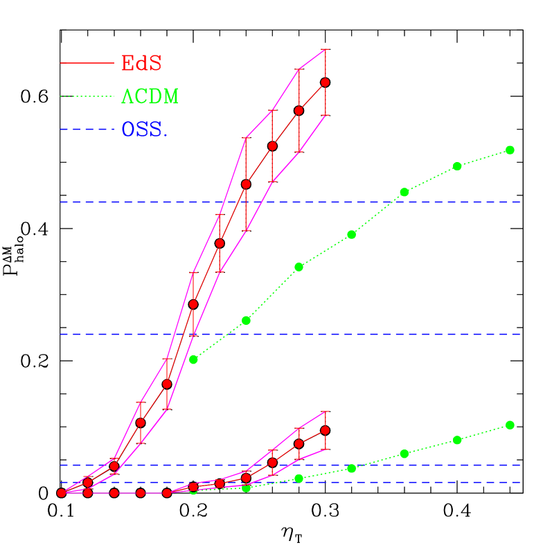
Figure 8: Expected formation probability of radio halos ($R_{H}\simeq 500h_{50}^{-1}$kpc, $B\sim 0.5\mu$G) as a function of parameter $\eta_{t}$ in a EdS cosmology (solid lines with error bars) and in a $\Lambda$CDM cosmology (dotted lines) in the mass bins: binA=$[1.8-3.6]\,10^{15}M_{\odot}\,h_{50}^{-1}$ and binB=$[0.9-1.8]\,10^{15}M_{\odot}\,h_{50}^{-1}$ for EdS case and binA=$[1.9-3.8]\cdot 10^{15}$ M_⊙h${}_{70}^{-1}$ and binB=$[0.945-1.9]\cdot 10^{15}$ M_⊙h${}_{70}^{-1}$ for the $\Lambda$CDM model. The two bottom dashed lines mark the observed probabilities for radio halos in the mass binB while the two top dashed lines mark the observed probabilities in the mass binA; observational regions account for 1$\sigma$ errors.

Following the procedures adopted in the case of the EdS cosmology, we compute merger trees (Sect. 3), turbulence injection rate and spectrum of the MS waves (Sect. 4), particle evolution (Sect. 5) and non-thermal emission (Sect. 6) from galaxy clusters and thus the expected formation probability of radio halos for $z<0.2$ (Sect. 7). In Fig.8, we report the comparison between the probability to form radio halos obtained in the two cosmologies. The comparison is derived by converting the virial mass of the clusters from a EdS into a $\Lambda$CDM model:

$$M_{v}^{\Lambda}=M_{v}^{EdS}\times\bigg{(}{{[\Delta_{c}(t)\rho_{m}(t)]_{EdS}}\over{[\Delta_{c}(t)\rho_{m}(t)]_{\Lambda}}}\bigg{)}^{1/2}$$ (59)

where $\rho_{m}$ is the mean mass density (dark and barionic) of the Universe. Thus the calculations with a $\Lambda$CDM model are performed for the mass bins $[0.945-1.9]\cdot 10^{15}$ M_⊙h${}_{70}^{-1}$ and $[1.9-3.8]\cdot 10^{15}$ M_⊙h${}_{70}^{-1}$.

As expected, we find that at $z<0.2$ the results are relatively independent from the considered cosmology, with the $\Lambda$CDM model being only slightly less efficient. In particular, as in the EdS case we note that it is possible to find a unique interval in $\eta_{t}$ in which the model reproduces the observed halo formation probability for both the cluster-mass bins.

In the $\Lambda$CDM Universe the structures start to grow at early time with respect to the EdS case, the merging rate at $z<0.2$ is consequently reduced, and thus particle acceleration is less efficient. However, this is roughly compensated by the fact that in a $\Lambda$CDM Universe the observed radio halos are smaller and less luminous than in the EdS case.

Appendix B Turbulence injection at a single scale

In this Appendix we adopt the scenario in which MHD turbulence is injected in the ICM at a large single–scale, $k_{min}\sim\pi/r_{s}$, from which the MHD turbulence cascade is originated.

The mean free path, $L_{mfp}$, in the ICM marks the boundary between the collisionless regime ($k>2\pi/L_{mfp}$) and the collisional regime ($k<2\pi/L_{mfp}$). It is given by (e.g., Braginskii 1965):

$$L_{mfp}({\rm kpc})\sim 300({{T}\over{10^{8}}})^{2}({{n_{th}}\over{10^{-4}}})^{-1}$$ (60)

which, for the typical values of the cluster temperatures and of the mean thermal density within $V_{H}$, is of the order of 100 kpc.

Once MS waves are injected at $k_{min}$, the process of wave–wave coupling generates a turbulence cascade. The cascade time of fast MS waves at the wavenumber $k$ is given by (e.g., Yan & Lazarian 2004):

$$\tau_{kk}(k)\sim{{v_{M}}\over{kv_{k}^{2}}}\sim{{v_{M}\rho}\over{k^{2}W_{k}}}$$ (61)

so that the diffusion coefficient in Eq.(22) is given by :

$$D_{kk}\sim{{k^{2}}\over{\tau_{kk}}}\sim{{v_{A}^{2}}\over{v_{M}}}{{k^{4}W_{k}}\over{2W_{B}}}$$ (62)

In the quasi linear regime, the spectrum of the waves due to the cascading process can be calculated solving Eq.(22) and neglecting the contribution due to the damping terms :

$${{\partial W_{\rm k}(t)}\over{\partial t}}={{\partial}\over{\partial k}}\left(D_{\rm kk}{{\partial W_{\rm k}(t)}\over{\partial k}}\right)+I_{\rm k}$$ (63)

with $I_{\rm k}=I_{o}\delta(k-k_{min})$ and $I_{o}\simeq\eta_{t}v_{i}^{3}\rho(\pi r_{s}^{2}/V_{H})$ (Sect. 4.1). The stady state solution of Eq.(63) is a Kraichnan–like spectrum :

$$W_{\rm k}\simeq\left({{2\rho I_{o}v_{M}}\over{3}}\right)^{1/2}k^{-3/2}$$ (64)

This spectrum extends down to a truncation scale at which the cascading time, $\tau_{kk}$, becomes substantially larger (i.e., $\xi$ times, $\xi\sim 1-3$) than the damping time scale, $\tau_{d}\sim\Gamma_{th,e}^{-1}$ (Eq. 23). In the collisionless regime, this truncation scale, $L_{tr}\sim 2\pi/k_{tr}$, is obtained from Eqs.(23), (62), and (64), one has :

$$L_{tr}\simeq{{0.23}\over{\xi^{2}\eta_{t}}}({{T}\over{10^{8}}})^{3/2}({{v_{i}}\over{10^{3}{\rm km/s}}})^{-3}\left({4\over 3}{{R_{H}^{3}}\over{r_{s}^{2}}}\right)$$ (65)

which typically falls in the range 10–30 kpc for our synthetic clusters (note that such scale is smaller than $L_{mfp}$ and thus the estimate can be done under the assumption of a collisionless regime), i.e. a factor of 30–100 smaller than the value of the typical turbulence injection scale (Sect. 4.1-4.2, Fig. 3b).

The picture of the model in this Appendix is thus that the injection of MHD turbulence occurs at a maximum scale of the order of 1 Mpc which is larger but relatively close to the scales typical of the collisionless regime. The wave-wave coupling then leads to a power-law inertial range with a Kraichnan spectrum which is approximatively mantained down to $\sim 10-30$ kpc. At these scales the damping time with the thermal electrons becomes considerably shorter than the cascading time–scale and the turbulence cascade is broken.

Under these conditions the acceleration time of relativistic electrons, $\tau_{\rm acc}$, is dominated by the contribution from the spectrum of the waves at the truncation scale and it can be obtained from Eqs.(41) and (42) :

$$\tau_{\rm acc}^{-1}=\chi\propto v_{M}^{2}W_{k}(k=k_{tr})k_{tr}^{2}$$ (66)

An important point is to check if the scenario adopted in Sect. 4 and that adopted in this Appendix give consistent results. In the scenario adopted in Sect. 4.2, the spectrum of the MS waves is approximately given by :

$$W_{k}\sim I_{k}\tau_{d}(k)$$ (67)

and thus, since $I_{o}=\int I_{k}dk$ and the damping time scale is $\tau_{d}(k)\sim\Gamma_{e,th}^{-1}\propto k^{-1}$, one has :

$$D_{pp}\sim c_{pp}\int W_{k}kdk\sim I_{o}\tau_{d}(k_{tr})k_{tr}$$ (68)

where $c_{pp}$ does not depend on the turbulence spectrum and energy (Eq. 41). On the other hand, in the scenario adopted in this Appendix the spectrum of the MS waves is approximately given by :

$$W_{k}\sim{{I_{o}}\over{k}}\tau_{kk}$$ (69)

and thus, since the cascading time scale is $\tau_{kk}\propto k^{-1/2}$, one has :

$$D_{pp}\sim c_{pp}\int W_{k}kdk\sim 2\,I_{o}\tau_{kk}(k=k_{tr})k_{tr}$$ (70)

as a consequence, since $k_{tr}$ is the scale at which the damping time scale and the cascading time scale are comparable, we expect that the two scenarios would provide a similar acceleration efficiency.

More specifically, we can calculate the electron acceleration coefficient due to a single merger event (with $r_{s}\geq R_{H}$) in the framework of the scenario adopted in this Appendix. From Eqs.(64), (65), (66), (9), and the expression for $I_{o}$ given in this Appendix, one finds :

$$\chi\sim 2\times 10^{-16}\xi\eta_{t}\left({{M}\over{2\times 10^{15}M_{\odot}}}\right)^{3/2}\left({{kT}\over{7\,keV}}\right)^{-1/2}\left[{{(r_{s}/500kpc)^{2}}\over{(R_{H}^{3}/500kpc)}}\right]$$ (71)

which is close to the value given in Eq.(49), and thus proves that the main results of our model do not crucially depend on the assumptions on the specific injection process (and spectrum) of the MS waves.

Appendix C Synchrotron and IC Radiation

In this Appendix we briefly describe the formalism adopted to calculate the synchrotron and IC emission from galaxy clusters.

The synchrotron emissivity is given by:

$$J_{syn}(\nu,t)=\frac{\sqrt{3}e^{3}B}{mc^{2}}\int_{p}\int_{0}^{\pi/2}dpd\theta sin^{2}\theta N(p,t)F(\frac{\nu}{\nu_{c}})$$ (72)

where $F(\frac{\nu}{\nu_{c}})$ is the synchrotron Kernel given by (e.g., Rybicki & Lightman, 1979):

$$F(\frac{\nu}{\nu_{c}})=\frac{\nu}{\nu_{c}}\int_{\nu/\nu_{c}}^{\infty}K_{\frac{5}{3}}(y)dy$$ (73)

with $\nu_{c}=(3/4\pi)p^{2}eBsin\theta/(mc)^{3}$.

The IC emissivity due to the scattering off the CMB photons by relativistic electrons is given by (e.g., Blumenthal & Gould,1970):

$$J_{IC}(\nu_{1},t)=(2\pi r_{o}m^{2}c)^{2}h\nu_{1}^{2}\int_{\nu}\int_{p}d\nu dp\frac{N(p,t)p^{-4}}{exp(\frac{h\nu}{k_{B}T_{z}})-1}\times{}$$ (74)

$${}(1+2\ln(\frac{\nu_{1}m^{2}c^{2}}{4p^{2}\nu})+\frac{4p^{2}\nu}{m^{2}c^{2}\nu_{1}}-\frac{m^{2}c^{2}\nu_{1}}{2p^{2}\nu})$$

where $T_{z}=2.73(1+z)$ is the temperature of the CMB photons.

References

- [1] Arnaud M., Evrard A.E., 1999, MNRAS 305, 631
- [2] Bahcall N.A., Fan X., 1998, ApJ 504,1
- [3] Barnes A., Scargle J.D., 1973, ApJ 184, 251
- [4] Berezinsky V.S., Blasi P., Ptuskin V.S., 1997, ApJ 487, 529
- [5] Berrington R. C., Dermer C. D., 2003, ApJ 594, 709
- [6] Biermann P.L., Enßlin T.A., Kang H., Lee H., Ryu D., 2003, in ’Matter and Energy in Clusters of Galaxis’, ASP Conf. Series, vol.301, p.293, eds. S. Bowyer and C.-Y. Hwang
- [7] Blasi P., 2001, APh 15, 223
- [8] Blasi P., 2003, in ‘Matter and Energy in Clusters of Galaxis’, ASP Conf. Series, vol.301, p.203, eds. S. Bowyer and C.-Y. Hwang
- [9] Blasi P., Colafrancesco S., 1999, APh 12, 169
- [10] Blumenthal G.R., Gould R.J.,1970, Reviews of Modern Physics, vol. 42, Issue 2, pp. 237-271
- [11] Borovsky J.E., Eilek J.A., 1986, ApJ 308, 929
- [12] Braginskii S.I., 1965, Rev. Plasma Phys. 1, 205
- [13] Brunetti G., 2003, in ’Matter and Energy in Clusters of Galaxis’, ASP Conf. Series, vol.301, p.349, eds. S. Bowyer and C.-Y. Hwang
- [14] Brunetti G., Setti G., Feretti L., Giovannini G., 2001a, MNRAS 320, 365
- [15] Brunetti G., Setti G., Feretti L., Giovannini G., 2001b, New Astronomy 6, 1
- [16] Brunetti G., Blasi P., Cassano R., Gabici S., 2004, MNRAS, 350, 1174
- [17] Cavaliere, A.; Fusco-Femiano, R, 1976, A&A, 49, 137.
- [18] Colafrancesco S., 1999, in ”Proceedings of the Workshop… Ringberg Castle, Germany, April 19-23, 1999”, Edited by H. Bohringer, L. Feretti, P. Schuecker., p.269, 274
- [19] Dennison B., 1980, ApJ 239L
- [20] Duffy P., 1994, ApJS 90, 981
- [21] Ebeling H., Voges W., Bohringer H., Edge A.C., Huchra J.P., Briel U.G., 1996, MNRAS 281, 799
- [22] Eilek J.A., 1979, ApJ 230, 373
- [23] Enßlin T.A., Biermann P.L., Kronberg P.P., Wu X.-P., 1997, ApJ 477, 560
- [24] Enßlin, T. A.; Rttgering, H., 2002, A&A, 396, 83
- [25] Enßlin, T. A., 2003, A&A 399, 409
- [26] Ettori S., Fabian A.C., 1999, MNRAS 305, 834
- [27] Feretti L., 2003, in ’Matter and Energy in Clusters of Galaxis’, ASP Conf. Series, vol.301, p.143, eds. S. Bowyer and C.-Y. Hwang
- [28] Fujita, Y.; Sarazin, C.L.,2001, ApJ, 563, 660.
- [29] Fujita Y., Takizawa M., Sarazin C.L., 2003, ApJ 584, 190
- [30] Fusco–Femiano R., Dal Fiume D., Feretti L., et al., 1999 ApJ 513, 197L
- [31] Fusco-Femiano R., Dal Fiume D., De Grandi S., 2000, ApJ 534, L7
- [32] Fusco-Femiano R.,Dal Fiume D., Orlandini M., De Grandi S., Molendi S., Feretti L., Grandi P., Giovannini G., 2003, in ‘Matter and Energy in Clusters of Galaxis’, ASP Conf. Series, eds., vol.301, p.109, S. Bowyer and C.-Y. Hwang
- [33] Fusco-Femiano R., Orlandini M., Brunetti G., Feretti L., Giovannini G., Grandi P., Setti G., 2004, ApJ 602, 73
- [34] Gabici S., Balsi P., 2003, ApJ 583, 695
- [35] Giovannini G., Tordi M., Feretti L., 1999, NewA 4, 141
- [36] Giovannini G., Feretti L., 2002 in ’Merging Processes in Galaxy Cluster’, vol.272, p.197, eds. L.Feretti, I.M.Gioia, G.Giovannini
- [37] Govoni, F.; Feretti, L.; Giovannini, G.; Bö hringer, H.; Reiprich, T. H.; Murgia, M. 2001, A&A, 376, 803
- [38] Jaffe W.J., 1977, ApJ 212, 1
- [39] Kempner J.C., Sarazin C.L., 2001, ApJ 548, 639
- [40] Kitayama T., Suto Y., 1996, ApJ.469, 480
- [41] Kuo, P.-H.; Hwang, C.-Y.; Ip, W.-H., 2004, ApJ 604, 108
- [42] Lacey, C., Cole S., 1993, MNRAS 262, 627
- [43] Liang H., Hunstead R.W., Birkinshaw M., Andreani P., 2000, ApJ 544, 686
- [44] Markevictch M., Vikhlinin A., Forman W.R., 2003, in ’Matter and Energy in Clusters of Galaxis’, ASP Conf. Series, vol.301, p.37, eds. S. Bowyer and C.-Y. Hwang
- [45] Melrose D.B., 1968, ApSS 2, 171
- [46] Miller J.A., LaRosa T.N., Moore R.L., 1996, ApJ 461, 445
- [47] Miniati F., 2002, MNRAS 337, 199
- [48] Miniati F., to appear in the proceedings of “Modelling the Intergalactic and Intracluster Media”, Vulcano Island, October 1-4, 2003, astro-ph/0401478
- [49] Miniati F., Ryu D., Kang H., Jones T. W., Cen R., Ostriker J. P., 2000, ApJ 542, 608
- [50] Miniati F., Jones T.W., Kang H., Ryu D., 2001, ApJ 562, 233
- [51] Nevalainen, J., Markevitch, M., Forman, W., 2000, ApJ 532, 694
- [52] Ohno H. Takizawa M., Shibata S., 2002, ApJ 577, 658
- [53] Peebles, P.J.E., 1980, ’The Large Scale Structure of the Universe’, edited by Peebles, P.J.E. The Princeton Univ. Press, Princeton, NJ.
- [54] Petrosian V., 2001, ApJ 557, 560
- [55] Press W.H., Schechter P., 1974, ApJ 187, 425
- [56] Randall S.W., Sarazin C.L., Ricker P.M., 2002, ApJ 577, 579
- [57] Rephaeli Y., Gruber D., Blanco P., 1999, ApJL 511, 21
- [58] Rephaeli Y., Gruber D., 2002, ApJ 579, 587
- [59] Rephaeli Y., Gruber D., 2003, ApJ 595, 137
- [60] Ricker P.M., Sarazin C.L., 2001, ApJ 561, 621
- [61] Roettiger K., Loken C., Burns J.O., 1997, ApJ 109, 307
- [62] Roettiger K., Burns J.O., Stone J.M., 1999, ApJ 518, 603
- [63] Rossetti M., Molendi S., 2004, A&A 414, 41
- [64] Ryu D., Kang H., Hallman E., Jones T.W., 2003, ApJ 593, 599
- [65] Rybicki G.B., Lightman A.P., 1979, ’Radiative Processes in Astrophysics’, Wiley, New York
- [66] Salvador-Sole E., Solanes J.M., Manrique A., 1998, ApJ 499, 542
- [67] Sarazin C.L., 1999, ApJ 520, 529
- [68] Sarazin C.L., 2002, in ‘Merging Processes in Clusters of Galaxies’, vol.272, p.1, edited by L. Feretti, I. M. Gioia, and G. Giovannini
- [69] Schlickeiser R., Sievers A., Thiemann H., 1987, A&A 182, 21
- [70] Schuecker P., Finoguenov A., Miniati F., Boehringer H., Briel U.G., 2004, A&A 426, 387
- [71] Sheth R.K., Tormen G., 1999, MNRAS 308, 119
- [72] Somerville, R. S.; Kolatt, T. S., 1999, MNRAS, 305, 1
- [73] Sunyaev, R. A., Norman, M. L., Bryan, G. L., 2003, Astronomy Letters, vol. 29, p. 783-790
- [74] Takizawa M., Naito T., 2000, ApJ 535, 586
- [75] Tormen G., Moscardini L., Yoshida N., 2004, MNRAS 350, 1397
- [76] Tsytovich V.N., 1966, Soviet Phys. Uspekhi 9, 370
- [77] Völk H.J., Aharonian F.A., Breitschwerdt D., 1996, SSRv 75, 279
- [78] Völk H.J., Atoyan A.M., 1999, APh 11, 73
- [79] Yan H., Lazarian A., 2004, ApJ 614, 757