A layered model for non-thermal radio emission
from single O stars

We present a model for the non-thermal radio emission from bright O stars, in terms of synchrotron emission from wind-embedded shocks. The model is an extension of an earlier one, with an improved treatment of the cooling of relativistic electrons. This improvement limits the synchrotron-emitting volume to a series of fairly narrow layers behind the shocks. We show that the width of these layers increases with increasing wavelength, which has important consequences for the shape of the spectrum. We also show that the strongest shocks produce the bulk of the emission, so that the emergent radio flux can be adequately described as coming from a small number of shocks, or even from a single shock.

A single shock model is completely determined by four parameters: the position of the shock, the compression ratio and velocity jump of the shock, and the surface magnetic field. Applying a single shock model to the O5 If star Cyg OB2 No. 9 allows a good determination of the compression ratio and shock position and, to a lesser extent, the magnetic field and velocity jump.

Our main conclusion is that strong shocks need to survive out to distances of a few hundred stellar radii. Even with multiple shocks, the shocks needed to explain the observed emission are stronger than predictions from time-dependent hydrodynamical simulations.

1 Introduction

About one quarter of the brightest O stars have a detectable radio flux of non-thermal origin, in addition to their thermal radio emission (Bieging et al. BAC89 (1989)). The thermal radio emission is due to free-free emission in the stellar wind (Wright & Barlow WB75 (1975)), whereas the non-thermal radiation is probably synchrotron emission by shock-accelerated electrons (White W85 (1985)). Usually, the thermal emission is only a small fraction of the flux, and the non-thermal emission dominates at centimetre wavelengths.

In a previous paper (Van Loo et al. VL04 (2004), hereafter Paper I) we used a phenomenological model to explain the observed spectrum of the O5 If star Cyg OB2 No. 9. The synchrotron-emitting electrons are assumed to be accelerated by wind-embedded shocks, such as those produced by the instability of the radiative driving mechanism. A power law was assumed for the momentum distribution of the electrons and the synchrotron-emitting volume was assumed to extend to an outer boundary $R_{\rm max}$. This approach leads to a model with a small number of free parameters, all of which are well-determined by the fit to the observations. Particularly, the interplay between non-thermal emission and thermal absorption places a firm constraint on the outer boundary $R_{\rm max}$.

In Paper I, the spatial distribution of the relativistic electrons was given by a power law. This implies that the radiation is emitted by a continuous volume extending out to $R_{\rm max}$. In the present paper, we take a closer look at this assumption. In the shock-acceleration mechanism discussed in Paper I (first order Fermi acceleration, Bell B78 (1978)) electrons are accelerated to relativistic energies by making many round-trips over the shock. Relativistic electrons are subject to a number of cooling mechanisms, most notably inverse Compton scattering in the presence of a dense radiation field (Chen C92 (1992)). They may therefore lose their energy rather fast when they eventually escape downstream and move away from the shock. In this case the emission is not expected to come from a continuous volume, but rather from a number of (possibly thin) layers behind the shocks.

Hydrodynamical models (e.g. Runacres & Owocki RO04 (2004)) of instability-generated shocks show a wide variety of shock strengths (both in velocity jump and compression ratio). We find that the strongest shocks generate most of the synchrotron emission, which means that the number of layers responsible for the observed synchrotron emission can actually be quite small.

In the following, we first (Sect. 2) derive the momentum distribution of relativistic electrons in the presence of cooling and discuss the effect on the emergent flux. In Sect. 3, we then apply a model where the emission is concentrated in a small number of thin layers to radio observations of the same star which was used in Paper I, Cyg OB2 No. 9. Finally (Sect. 4), we discuss the implications of our results and draw some conclusions.

2 Emission layers

2.1 Momentum distribution at the shock front

Electrons are accelerated at a shock by the first order Fermi acceleration (Bell B78 (1978)). Every time an electron crosses the shock front, it gains a small amount of momentum. When an electron is kept in the vicinity of the shock front and crosses the shock front many times, it can be accelerated to relativistic momenta. The acceleration rate of the Fermi mechanism is given by

$$\frac{{\rm d}p}{{\rm d}t}=\frac{\Delta p}{\Delta t_{\rm cycle}},$$ (1)

where

$$\Delta p=\frac{4}{3}\frac{\Delta u}{c}p,$$ (2)

is the momentum gain for an electron per round-trip. The round-trip time $\Delta t_{\rm cycle}$ can be determined as follows. After crossing the shock, a typical electron travels a mean free path $\lambda=pc/eB$ (White W85 (1985)), where $B$ is the magnetic field and other symbols have their usual meaning, before it is scattered by magnetic irregularities. An electron does not necessarily return to the shock after one scattering. From Lagage & Cesarsky (LC83 (1983)) we derive that an electron is scattered $c/2u$ times before recrossing the shock, where $u$ is the speed of the bulk motion upstream ($u_{1}$) or downstream ($u_{2}$) of the shock (both measured in the shock frame). Since the time between scattering events is given by $2\lambda/c$, the time needed for an electron to cross the shock is $\lambda/u$. Therefore the round-trip time is given by (Lagage & Cesarsky LC83 (1983))

$$\Delta t_{\rm cycle}=\frac{\lambda}{u_{1}}+\frac{\lambda}{u_{2}}.$$ (3)

For a shock with a compression ratio $\chi=u_{1}/u_{2}$ and a velocity jump $\Delta u=u_{1}-u_{2}$, the speeds (measured in the shock frame) are given by

$$u_{1} = \frac{\chi\Delta u}{\chi-1},$$

$$u_{2} = \frac{\Delta u}{\chi-1}.$$ (4)

Then

$$\Delta t_{\rm cycle}=\frac{pc}{eB}\frac{\chi^{2}-1}{\chi\Delta u}.$$ (5)

The round-trip time $\Delta t_{\rm cycle}$ given in Eq. (3) is different from the expression $\Delta t_{\rm cycle}=2\lambda/c$ given by Chen (C92 (1992)). As this is the expression for the mean time between scatterings, the underlying assumption in Chen (C92 (1992)) is that the electron returns to the shock after one scattering.

Electrons are accelerated to high momenta, but also lose their momentum via different energy loss mechanisms. By taking the cooling into account, the net momentum gain rate of the acceleration process is drastically reduced. At the high momentum end of the spectrum, electrons are mainly cooled by the inverse-Compton scattering of photospheric UV photons at a rate (Rybicki & Lightman RL79 (1979))

$$\left(\frac{{\rm d}p}{{\rm d}t}\right)_{\rm IC}=-\frac{\sigma_{\rm T}L_{*}}{3\pi r^{2}c}\left(\frac{p}{m_{\rm e}c}\right)^{2},$$ (6)

where $\sigma_{\rm T}$ is the Thomson cross section, $L_{*}$ the stellar luminosity and $r$ is the distance from the star.

The net momentum gain per time interval due to first order Fermi acceleration and inverse-Compton cooling is then given by

$$\left(\frac{{\rm d}p}{{\rm d}t}\right)_{\rm net}=\left(\frac{{\rm d}p}{{\rm d}t}\right)_{\rm acc}+\left(\frac{{\rm d}p}{{\rm d}t}\right)_{\rm IC}.$$ (7)

The highest momentum attainable for relativistic electrons is determined by the balance between acceleration and inverse-Compton cooling at the shock. The result is a high momentum cut-off $p_{c}$ given by

$$p_{c}=m_{\rm e}c\left[\frac{\chi\Delta u^{2}}{\chi^{2}-1}\frac{4\pi R_{*}^{2}}{\sigma_{\rm T}L_{*}}\frac{eB_{*}}{c}\frac{v_{\rm rot}}{v_{\infty}}\frac{r}{R_{*}}\right]^{1/2},$$ (8)

where $R_{*}$ is the stellar radius, $v_{\rm rot}$ the rotational velocity of the star and $v_{\infty}$ the terminal velocity of the stellar wind and where we used $B=B_{*}\frac{v_{\rm rot}}{v_{\infty}}\frac{R_{*}}{r}$ (Weber & Davis WD67 (1967)). Using typical hot-star values ($L_{*}=10^{6}\leavevmode\nobreak\ {\rm L_{\odot}}$, $v_{\infty}=2\,500\leavevmode\nobreak\ {\rm km\,s^{-1}}$, $v_{\rm rot}=200\leavevmode\nobreak\ {\rm km\,s^{-1}}$, $R_{*}=20\leavevmode\nobreak\ {\rm R_{\odot}}$ and $\Delta u=100\leavevmode\nobreak\ {\rm km\,s^{-1}}$), we can estimate a numerical value for the high momentum cut-off,

$$p_{c}\approx\frac{15\leavevmode\nobreak\ {\rm MeV}}{c}\sqrt{\frac{B_{*}\chi}{\chi^{2}-1}\frac{r}{R_{*}}}.$$ (9)

Note that $p_{c}$ increases further out in the wind, due to the rapid depletion of UV photons. The high momentum cut-off is also weakly dependent on the compression ratio. Electrons can attain higher momenta in weak shocks, because the acceleration rate is higher in these shocks, as can be seen from Eqs. (1) and (5). The high momentum cut-off is a factor of $\sqrt{c/\Delta u}\approx 30$ lower than the value derived in Chen (C92 (1992)) and in Paper I, due to the different expressions for $\Delta t_{\rm cycle}$ (Eq. (5)).

In the absence of cooling, the acceleration of electrons through first order Fermi acceleration results in a power law momentum distribution (Bell B78 (1978)). When cooling is taken into account, the momentum distribution can be quite different from the power law. Near the high momentum cut-off, the net momentum gain goes to zero and the distribution will deviate from a pure power law. At low momenta, however, the acceleration rate is much higher than the cooling rate, so the momentum distribution is still a power law. Chen (C92 (1992)) showed that the spectrum including Compton cooling can be expressed as

$$N(p)=N_{E}p^{-n}\left(1-\frac{p^{2}}{p_{c}^{2}}\right)^{(n-3)/2},$$ (10)

where

$$n=\frac{\chi+2}{\chi-1},$$ (11)

and $N_{E}$ is a normalisation constant related to the energy density of the relativistic electrons (see below). The shape of the distribution is shown by the thick solid line in Fig. 1. The hook at the high momentum cut-off corresponds to the accumulation of electrons that, in the absence of cooling, would have had momenta above $p_{c}$. (A downward hook corresponding to the depletion of very energetic electrons can also occur. For a detailed explanation see Van Loo (Sven (2005)).) As the shape of the momentum distribution does not depend on the round trip time, Eq. (10) is unchanged from Chen (C92 (1992)).

We determine the normalisation constant $N_{E}$ by specifying the amount of energy that goes into the relativistic electrons. Following Ellison & Reynolds (ER91 (1991)), we assume that the relativistic electrons contribute little to the overall momentum balance across a shock. This means that the pressure of the relativistic electrons is only a small fraction ($\zeta$) of the total pressure difference. It is unlikely that $\zeta$ is more than 0.05 and it could be conceivably less (Blandford & Eichler BE87 (1987); Eichler & Usov EU93 (1993)). From the Rankine-Hugoniot relations we find that the pressure difference across the shock is

$$\Delta P=\rho_{1}\frac{\chi}{\chi-1}(\Delta u)^{2}.$$ (12)

Here $\rho_{1}$ is the density of the preshock gas. For simplicity we assume $\rho_{1}=\dot{M}/4\pi r^{2}v_{\infty}$. The relativistic electron pressure is given by (White W85 (1985))

$$P_{\rm rel}=\frac{1}{3}U_{\rm rel}=\frac{1}{3}\int_{p_{0}}^{p_{c}}{{\rm d}p\,pcN(p)},$$ (13)

with $U_{\rm rel}$ the energy density of the relativistic electrons and $p_{0}$ the low momentum cut-off. For reasons that will become apparent in Sect. 3.3.3, we set $\zeta$ equal to 0.05 (as opposed to $\zeta\leq 0.05$). Using Eqs. (12) and (13), we can then determine $N_{E}$.

The normalisation of the momentum distribution differs from the one used in Paper I, which was based on the relativistic number density being smaller than the total electron number density. For a given momentum distribution, the total number of relativistic electrons and the total energy are of course directly related. A constraint on one implies a constraint on the other. The energy constraint is, in principle, the more stringent as it is reached well before all electrons become relativistic.

2.2 Momentum distribution behind the shock front

Once an electron leaves the shock front, the acceleration ceases and cooling mechanisms will reduce its momentum. This means that the momentum distribution of relativistic electrons behind the shock will differ from the distribution observed at the shock. To describe the distribution behind the shock, we need to know where the electrons were accelerated and how their momentum is changed under the influence of cooling.

While the shock travels through the stellar wind with approximately the terminal speed $v_{\infty}$, the relativistic electrons will move away from the shock front with the gas, at a significantly lower speed $u_{2}$ (see Eq. (2.1)). This means that outer wind electrons may well have been accelerated in the inner wind. If the shock is at $R_{\rm S}$, the distribution of electrons at radius $r$, close to $R_{\rm S}$, was initially accelerated when the shock was at

$$r_{\rm i}=R_{\rm S}-v_{\infty}\frac{|R_{\rm S}-r|}{u_{2}}<R_{\rm S},$$ (14)

where we have assumed that $v_{\infty}$ and $u_{2}$ are constant throughout the wind. This expression is valid for both forward shocks (which move outward through the gas) and reverse shocks (which move inward through the gas). The momentum distribution produced at $r_{\rm i}$ is given by Eq. (10) with $p_{c}$ and $N_{E}$ evaluated at $r_{\rm i}$.

Once we know where the electrons are accelerated, we only need to take into account the cooling of the electrons. Inverse-Compton cooling, adiabatic cooling, synchrotron cooling and Bremsstrahlung cooling can all play a rôle. Since the observable radio emission comes from electrons with momenta of the order $\sim$ 100 MeV/c (see Paper I), we will only incorporate the cooling mechanisms which act at these momenta and higher. At high momenta, the electrons are mainly cooled by inverse-Compton cooling which dominates over synchrotron cooling (Chen C92 (1992)). For electrons with intermediate momenta, the adiabatic cooling is more important than Bremsstrahlung (Chen C92 (1992)). We will therefore include only inverse-Compton and adiabatic cooling.

The cooling rate of the relativistic electrons is not only dependent on the momentum of the electrons, but also changes with distance. Since the relativistic electrons move along with the thermal gas, we will express the cooling rate as the loss of momentum over a distance ${\rm d}r$, where we take ${\rm d}r=v_{\infty}{\rm d}t$. The cooling rate for relativistic electrons is then given by (e.g. Chen C92 (1992))

$$\frac{{\rm d}p}{{\rm d}r}=-a_{\rm ic}\frac{p^{2}}{r^{2}}-\frac{2}{3}\frac{p}{r},$$ (15)

where the first term represents the inverse-Compton cooling with $a_{\rm ic}=\sigma_{T}L_{*}/(3\pi m_{\rm e}^{2}c^{3}v_{\infty})$ and the second term the adiabatic cooling. An electron which was initially at $r_{\rm i}$ with momentum $p_{\rm i}$ will be cooled down to a momentum (Chen C92 (1992))

$$p=\frac{p_{\rm i}\left(\frac{r_{\rm i}}{r}\right)^{2/3}}{1+\frac{3a_{\rm ic}}{5}\frac{p_{\rm i}}{r_{\rm i}}\left[1-\left(\frac{r_{\rm i}}{r}\right)^{5/3}\right]},$$ (16)

when it reaches $r$.

The above expression enables us to determine the momentum distribution after cooling. We assume that a shock is spherically symmetric, i.e. that it covers a complete solid angle. The number of relativistic electrons initially having a momentum between $p_{\rm i}$ and $p_{\rm i}+{\rm d}p_{\rm i}$ at a radius $r_{\rm i}$ is then $4\pi r_{\rm i}^{2}N(p_{\rm i}){\rm d}p_{\rm i}{\rm d}r$, with $N(p)$ the differential number distribution given by Eq. (10) and $4\pi r^{2}_{\rm i}{\rm d}r$ the volume that contains the electrons. Inverse-Compton and adiabatic losses reduce the momentum of the electrons to values between $p$ and $p+{\rm d}p$ where $p$ is given by Eq. (16). Also, the volume of the shell expands to $4\pi r^{2}{\rm d}r$. Since the number of electrons in this momentum interval and volume is not changed, the number distribution after cooling $N_{c}(r,p)$ is given by

$$N_{c}(r,p)=N(p_{\rm i})\left(\frac{r_{\rm i}}{r}\right)^{2}\frac{{\rm d}p_{\rm i}}{{\rm d}p},$$ (17)

where $p_{\rm i}$ is given by the inverse function of Eq. (16). Eq. (17) is valid for all momenta lower than the momentum $p_{c,e}$, to which an electron that had a momentum $p_{c}$ at $r_{i}$ has cooled at $r$. Therefore, $p_{c,e}$ is given by Eq. (16) with $p_{i}=p_{c}$. Note that the momentum distribution at the shock front, $N(p)$ in Eq. (10), is given by $N_{c}(R_{S},p)$.

An example for the momentum distribution is given in Fig. 1. Here we plot the momentum distribution at the shock front for a strong shock ($\chi=4$ and $\Delta u=100\leavevmode\nobreak\ {\rm km\,s^{-1}}$) at $600\leavevmode\nobreak\ R_{*}$ and the momentum distributions which are found $1.5\leavevmode\nobreak\ R_{*}$, $3.0\leavevmode\nobreak\ R_{*}$ and $4.5\leavevmode\nobreak\ R_{*}$ behind the shock. These distributions were accelerated respectively at $470\leavevmode\nobreak\ R_{*}$, $339\leavevmode\nobreak\ R_{*}$ and $209\leavevmode\nobreak\ R_{*}$. It is clear that the highest attainable momentum drops off rather rapidly behind the shock: electrons which are $4.5\leavevmode\nobreak\ R_{*}$ behind the shock no longer contribute to the observable radio emission, i.e. the emission layer is no thicker than $4.5\leavevmode\nobreak\ R_{*}$.

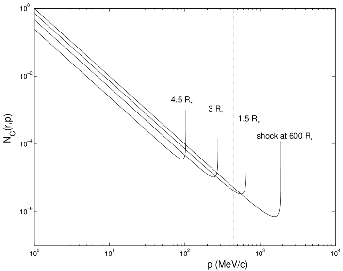
Figure 1: The cooling of relativistic electrons behind a strong shock ($\chi=4$ and $\Delta u=100\leavevmode\nobreak\ {\rm km\,s^{-1}}$). The thick solid line is the momentum distribution at the shock located at $600\leavevmode\nobreak\ R_{*}$. The three solid lines are the distributions away from the shock, at locations $600\leavevmode\nobreak\ R_{*}-1.5\leavevmode\nobreak\ R_{*}$, $600\leavevmode\nobreak\ R_{*}-3\leavevmode\nobreak\ R_{*}$ and $600\leavevmode\nobreak\ R_{*}-4.5\leavevmode\nobreak\ R_{*}$. We assumed $N(1\leavevmode\nobreak\ {\rm MeV/c})=1$ at $600\leavevmode\nobreak\ R_{*}$ and $B_{*}=100\leavevmode\nobreak\ {\rm G}$. The dashed lines indicate the momentum that the relativistic electrons must have to produce synchrotron radiation between 2 and 20 cm ($450\leavevmode\nobreak\ {\rm MeV/c}>p>140\leavevmode\nobreak\ {\rm MeV/c}$).

Eqs. (16) and (17) are valid for both reverse and forward shocks. The momentum distribution at a distance $|R_{S}-r|$ behind a reverse or forward shock is initially accelerated at $r_{i}$. Electrons with a momentum $p_{i}$ at $r_{i}$ are then cooled down to a momentum $p$ at $r$. Although $r$ is not the same for a reverse and forward shock, the momentum $p$ is not significantly different as long as $|R_{S}-r|\ll|R_{S}-r_{i}|$. Since this criterion is fulfilled for $u_{2}\ll v_{\infty}$, this means that a reverse and forward shock will have the same momentum distribution at a distance $|R_{S}-r|$ downstream of the shock. It is therefore possible to discuss only forward shocks in the rest of the paper without loss of generality.

2.3 Synchrotron emission layers

The previous section shows that the relativistic electrons (and thus also the synchrotron emission) are limited to narrow layers behind the shock. The width of the synchrotron emission layers is determined by the distance over which the relativistic electrons still produce observable radio emission. The emission at a given frequency produced by a distribution of relativistic electrons is given by (Paper I)

$$j_{\nu}(r)=\frac{1}{4\pi}\int_{p_{0}}^{p_{\rm c,e}}{{\rm d}p\,N_{c}(r,p)\bar{P}_{\nu}(r,p)},$$ (18)

where $\bar{P}_{\nu}(p)$ is the synchrotron power of a single electron averaged over solid angle. We take into account the Razin effect (Razin R60 (1960); see also Ginzburg & Syrovatskii GS65 (1965)), which is a plasma effect that greatly reduces the synchrotron emitting power.

Although the emissivity is calculated by integrating over all momenta, only electrons within a narrow range of momenta contribute to the emissivity at a given frequency. A relativistic electron with momentum $p$ emits most of its energy in a narrow region around the frequency (Ginzburg & Syrovatskii GS65 (1965))

$$\nu\approx 0.29\frac{3}{4\pi}\frac{eB}{m_{\rm e}c}\left(\frac{p}{m_{\rm e}c}\right)^{2}.$$ (19)

In a local magnetic field of $B=0.015\leavevmode\nobreak\ {\rm G}$ the synchrotron emission between 2 – 20 cm (15 – 1.4 GHz) is produced by electrons with momenta between 140 and 450 MeV/c. The emission at a given wavelength is thus related to a specific momentum and the emission layer extends up to the distance behind the shock where all relativistic electrons are below this momentum.

The width of the synchrotron emission layer $\Delta R_{S}$ is determined by the time $\Delta t_{\rm cool}$ to cool the relativistic electrons below radio emitting momenta. From Eq. (15) we see that the cooling rate decreases with distance from the star. This means that the relativistic electrons are cooled faster close to the star and that the width of the emission layer behind the shock is larger further out in the wind. The width is proportional to $\Delta t_{\rm cool}$. The cooling time $\Delta t_{\rm cool}$ in principle also depends on the value of the high momentum cut-off $p_{c}$, but this turns out to be a minor effect. Furthermore, the width of the emission layer is influenced by the outflow speed of the relativistic electrons. Because the relativistic electrons flow away from the shock with a velocity $u_{2}$ given in Eq. (2.1), the width of the emission layer is directly proportional to $u_{2}$.

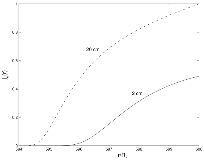
Figure 2: The emissivity behind a strong forward shock at $r=600\leavevmode\nobreak\ R_{*}$ for 2 different wavelengths. The dashed line is the emissivity at 20 cm and the solid line at 2 cm. We normalised the emissivity to the highest value.

An important point is that the width of the emission layers depends on wavelength. At short wavelengths the radiation is produced by more energetic electrons (Eq. (19)). Since these electrons are cooled more rapidly by inverse-Compton cooling (Fig. 1), the emission layers at shorter wavelengths are narrower, as can be seen in Fig. 2. These differences change the shape of the synchrotron spectrum (Sect. 2.6). The emission layers in Fig. 2 are somewhat larger than expected from Fig. 1, because the emission at a given wavelength is produced by electrons, not with one specific momentum, but within a narrow momentum range.

2.4 Emergent flux

The emergent synchrotron flux of an electron distribution behind a shock is given by

$$F_{\nu}=\frac{1}{D^{2}}\int_{R_{S}-\Delta R_{S}(\nu)}^{R_{S}}{{\rm d}r4\pi r^{2}j_{\nu}(r)G\left(\frac{r}{R_{\nu}}\right)},$$ (20)

where $D$ is the distance to the star, $R_{\nu}$ the characteristic radius of emission (Wright & Barlow WB75 (1975)), $\Delta R_{S}(\nu)$ the width of the emission layer at a frequency $\nu$ and $G(r/R_{\nu})$ a function that describes the influence of free-free absorption in the stellar wind (see Paper I). Because of the triangular shape of the synchrotron emissivity behind a shock (see Fig. 2), the synchrotron flux can be approximated, to first order, by

$$F_{\nu}\approx\frac{4\pi R^{2}_{S}}{D^{2}}\frac{j_{\nu}(R_{S})G\left(\frac{R_{S}}{R_{\nu}}\right)}{2}\Delta R_{S}(\nu).$$ (21)

All calculations are done using the exact expression Eq. (20), but this approximate expression is useful in the discussions of the following sections.

The synchrotron radio fluxes emitted behind a shock given in Eq. (20) can be calculated numerically. In the code (which is similar to the one used in Paper I), the momentum integral of the emissivity, given in Eq. (18), is computed using the trapezoidal rule and the step size is refined until it reaches a desired fractional precision of $10^{-3}$. The emissivity has to be calculated at different positions behind the shock. Then, the spatial integral of the flux, Eq. (20), is treated in the same way as the momentum integral, but up to a precision of order 1%. Here the function $G(r/R_{\nu})$ is determined using a linear interpolation between precalculated values. The number distribution is given by Eq. (17), while the mean synchrotron power of a single electron $\bar{P}_{\nu}$ is determined using precalculated values in the same way as $G(r/R_{\nu})$. We included the Razin effect in the calculation of $\bar{P}_{\nu}$ (see Paper I). The low momentum cut-off is assumed $p_{0}=1\leavevmode\nobreak\ {\rm MeV/c}$, while the high momentum cut-off $p_{c,e}$ is found by evaluating Eq. (8) in Eq. (16).

The total emergent flux also has a contribution from free-free emission by thermal electrons. This contribution is calculated using the Wright & Barlow formalism (Wright & Barlow WB75 (1975)) and added to the non-thermal flux.

2.5 Dominance of the strong shocks

Hydrodynamical simulations show that a hot-star wind is filled with shocks out to very large distances (Runacres & Owocki RO04 (2004)). These shocks exhibit a large variation in shock velocity jump and compression ratio. In this section we will show that the shocks with high $\chi$ and $\Delta u$ dominate the radio emission. Consequently, the shock distribution responsible for the observed emission corresponds to a few isolated shocks in the wind.

The normalisation constant $N_{E}$ of the momentum distribution is proportional to the pressure difference $\Delta P$ across the shock, which has a $\Delta u^{2}$-dependence. This means that the number of electrons in all momentum ranges increases with the shock velocity jump. Furthermore the synchrotron emissivity $j_{\nu}$, given by Eq. (18), is directly proportional to $N_{E}$ which means that the emissivity must be proportional to $\Delta u^{2}$. In Sect. 2.3 we showed that the width of the emission layer is also proportional to $\Delta u$. From Eq. (21) it then follows that the synchrotron flux is proportional to $\Delta u^{3}$. This relation remains valid if we use the exact expression Eq. (20) to calculate the synchrotron flux.

The radio fluxes do not only increase with the shock velocity jump, but also with the compression ratio $\chi$. The slope of the momentum distribution becomes shallower with higher $\chi$ (see Eq. (10)). Assuming that the number of relativistic electrons is the same near $p_{0}$ (i.e. $N_{E}$ independent of $\chi$), more electrons are then present in the momentum range important for observable radio emission. As the emissivity at a given wavelength is related to the number of electrons with a specific momentum, more emission is radiated by the strongest shocks. A complication arises because the normalisation constant $N_{E}$ actually decreases with $\chi$ (Sect. 2.1), thereby slightly counteracting the effect of the slope. However, this complication turns out to have a minor effect. A grid of models (discussed in Sect. 3.2) shows that the flux only fails to increase with increasing $\chi$ if the shock is close to the stellar surface and if at the same time the magnetic field is strong. Even in such cases the effect is limited to 20 % on the flux.

Thus, the shocks with the highest compression ratios and shock velocity jumps in the wind dominate the radio emission.

2.6 Interpretation of the spectral index

The broadening of the synchrotron emission layers toward longer wavelengths has consequences on the shape of the observed synchrotron flux: the spectral index $\alpha$ of the emission is steeper than expected. For the sake of clarity, we neglect the Razin effect and the free-free absorption in the discussion.

For a power-law momentum distribution of relativistic electrons with index $n$, the synchrotron emissivity $j_{\nu}$ is given by a power law in frequency with an exponent (Rybicki & Lightman RL79 (1979))

$$\tilde{\alpha}=\frac{1-n}{2}.$$ (22)

Eq. (21), with $G(R_{S}/R_{\nu})=1$, shows that the spectral index $\alpha$ of the synchrotron flux would equal $\tilde{\alpha}$ if the width of the emission layer were independent of frequency. But as the emission layers broaden toward longer wavelengths (see Sect. 2.3), the synchrotron flux increases at these wavelengths and the radio spectrum steepens. As a consequence the spectral index is lower than $(1-n)/2$.

In astrophysical applications the measured radio spectral index $\alpha$ is often used to estimate the compression ratio of the shock that accelerated the relativistic electrons (e.g. Chen & White CW94 (1994)). If we observe synchrotron emission with a radio spectral index $\alpha=-0.75$ then for a non-cooling model we would derive a compression ratio $\chi=3$ using $\alpha=\tilde{\alpha}$ and Eq. (11). However, taking into account cooling behind the shock, we find that the observed flux corresponds to a strong shock with $\chi=4$.

3 Application and results

3.1 Cyg OB2 No. 9: 21 Dec 1984 data

Table 1: Relevant stellar parameters for Cyg~OB2~No.~9 adopted in this paper. The numbers are taken from Bieging et al. (BAC89 (1989), BAC), Leitherer (L88 (1988), L) and Herrero et al. (HCVM99 (1999), HCVM).

Parameter		Ref.
$v_{\rm rot}\sin i\leavevmode\nobreak\ ({\rm km\leavevmode\nobreak\ s^{-1}})^{a}$	145	BAC
$T_{\rm eff}\leavevmode\nobreak\ ({\rm K})^{b}$	44 500	HCVM
$R_{*}\leavevmode\nobreak\ ({\rm R_{\sun}})$	22	HCVM
$d\leavevmode\nobreak\ ({\rm kpc})$	1.82	BAC
$v_{\infty}\leavevmode\nobreak\ ({\rm km\leavevmode\nobreak\ s^{-1}})$	2 900	L
$\dot{M}\leavevmode\nobreak\ ({\rm M_{\sun}\leavevmode\nobreak\ yr^{-1}})$	$2.0\times 10^{-5}$	L
$L_{*}\leavevmode\nobreak\ ({\rm L_{\sun}})$	$1.74\times 10^{6}$	HCVM

^a We follow White (W85 (1985)) in assuming that $v_{\rm rot}=250\leavevmode\nobreak\ {\rm km\leavevmode\nobreak\ s^{-1}}$, which is not in contradiction with the value for $v_{\rm rot}\sin i$.
^b The wind temperature is assumed to be $0.3$ times the stellar effective temperature (Drew D89 (1989)).

In Paper I we applied the continuous model to the non-thermal radio emitter Cyg~OB2~No.~9 (O5 If). Of all the observational radio data that are available for Cyg~OB2~No.~9, we used the 1984 Dec 21 observation with the VLA (Bieging et al. BAC89 (1989)) because of its detection of emission in three radio wavelength bands and the small error bars on the detection. However the error bars on the Cyg OB2 No. 9 observations listed by Bieging et al. (BAC89 (1989)) are surprisingly small (0.1 mJy). The error due to the flux calibration should already be 5 % of the observed flux for 2 cm observations and 2 % for 6 and 20 cm observations (Perley & Taylor Perley+Taylor03 (2003)), which translates to 0.29, 0.15 and 0.10 mJy at 2, 6 and 20 cm. We can therefore conclude that only the random errors (root-mean-square) were listed. If we include the calibration errors (absolute flux scale errors), we find: 5.7 $\pm$ 0.3 mJy (2 cm), 7.4 $\pm$ 0.2 mJy (6 cm) and 4.9 $\pm$ 0.14 mJy (20 cm).

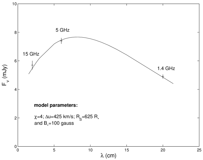
Figure 3: The VLA observations (21 Dec 1984) for Cyg~OB2~No.~9 with revised error bars. The solid line represents a single shock model that explains the non-thermal radio emission. The stellar parameters are given in Table 1.

A significant fraction of the radio emission is not radiated as synchrotron radiation by relativistic electrons, but is due to free-free emission from the stellar wind (Wright & Barlow WB75 (1975)). Using the values from Table 1, the contributions of the free-free emission to the observations of Cyg~OB2~No.~9 are: 1.4 mJy (2 cm), 0.7 mJy (6 cm) and 0.4 mJy (20 cm), if we assume that the stellar wind is completely ionised. The stellar parameters adopted are listed in Table 1. We will now apply a layered shock model to these observations of Cyg~OB2~No.~9.

3.2 Single shock model

The bulk of the emission by a set of shocks is produced by its strongest members (Sect. 2.5). To simplify the model further, we will consider the synchrotron emission from a single shock. The emission from multiple shocks can then be estimated by adding up the emission from single shock models (see Sect. 3.4). A single shock model is described by four parameters: the position of the shock $R_{S}$, the shock parameters $\Delta u$ and $\chi$ which determine the momentum distribution of the accelerated electrons and the surface magnetic field $B_{*}$. Hot stars are expected to have a surface magnetic field in the range of 10 to 200 G. The upper limit corresponds roughly to the detection limit of the field (no Zeeman splitting has been observed from any spectral line of any normal O star). The lower limit is set by the Razin effect, because otherwise no synchrotron radiation would be observed.

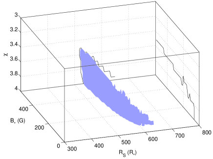
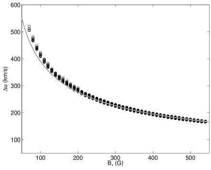
Figure 4: (a) Left panel: The combinations of $\chi$, $R_{\rm S}$ and $B_{*}$ that fit the observations for Cyg~OB2~No.~9 lie in the grey area on the figure. Projections on two planes are plotted to situate the solutions in the parameter space. (b) Right panel: For all possible combinations of the model parameters that explain the radio observations of Cyg~OB2~No.~9, the values for the surface magnetic field $B_{*}$ and the shock velocity jump $\Delta u$ are shown. The solid line represents $\Delta u^{3}B_{*}^{3/2}$ is constant.

Once a choice is made for the model parameters, we can calculate the synchrotron flux in the three wavelengths for a grid in $R_{\rm S}$, $\chi$, $\Delta u$ and $B_{*}$ and select those combinations of the parameters that fit the VLA observations within the error bars. The emergent flux for one such model is shown in Fig. 3. All possible combinations of $R_{\rm S}$, $\chi$, $\Delta u$ and $B_{*}$ are shown in Figs. 4a and 4b. Strong constraints are produced on all four parameters. In principle the ranges of the model parameters depend on $p_{0}$, but we checked that the effect is minimal.

3.3 Solution space

3.3.1 Compression ratio $\chi$ and shock position $R_{S}$

Fig. 4a shows that the shock parameters $R_{\rm S}$ and $\chi$ are rather precisely determined. If the observations are to be explained by a single shock, then it must be strong ($\chi=3.5-4$) and located between $520-640\leavevmode\nobreak\ R_{*}$.

The reason that we find strong shocks is as follows. The emission at 2 and 6 cm is barely influenced by the free-free absorption or the Razin effect (see below). In a simple analysis, this means that, at these wavelengths, the exponent $\tilde{\alpha}$ of the synchrotron emissivity is simply the radio spectral index $\alpha$. We can then derive the compression ratio of the shock directly from the radio spectrum. Using Eqs. (11) and (22), we then find $\chi=1-3/2\alpha$. (Note that this means that weaker shocks produce a steeper spectrum.) However, the steepening due to the wavelength dependence of the emission layer (see Sect 2.6) is not included in the above expression. This means that the compression ratio derived for a layered model will be larger than the compression ratio derived in the simple analysis above.

The shock responsible for the observed emission at 20 cm must be located at a large distance from the star, due to the large free-free absorption in the wind. All radio emission emitted too close to the star is absorbed and cannot be observed. This absorbing volume extends up to the radius $R_{\tau}(\nu)$ where the radial free-free optical depth is unity. Using $\int_{R_{\tau}(\nu)}^{\infty}{\chi_{\rm ff}{\rm d}r}=1$ with $\chi_{\rm ff}$ the free-free absorption coefficient given by Allen (A73 (1973)), we find

$$R_{\tau}(\nu)=1.76\times 10^{28}\left(\gamma g_{\nu}Z^{2}\right)^{1/3}T^{-1/2}\left(\frac{\dot{M}}{\mu v_{\infty}\nu}\right)^{2/3}{\rm cm},$$ (23)

where $T$ is in K, $\dot{M}$ in $M_{\sun}$/yr, $\nu$ in Hz and $v_{\infty}$ in ${\rm km\,s^{-1}}$ and where the other symbols have their usual meaning (Wright & Barlow WB75 (1975)). Thus, the synchrotron emission must be produced beyond $R_{\tau}({\rm 20\leavevmode\nobreak\ cm})$ which is $450\leavevmode\nobreak\ R_{*}$. Radiation emitted beyond this distance is not absorbed at 2 and 6 cm because the free-free opacity is smaller at shorter wavelengths. Although a shock is needed at large distances, it cannot be too far out in the wind. The free-free absorption at 20 cm would then be negligible, resulting in a pure power-law spectrum that does not explain the observations in Fig. 3.

The tight constraint on $R_{\rm S}$ presented here is only valid for a single shock. In Sect. 3.4, we will explain the observations by multiple shocks. These can be spread out over a fairly large geometric region, and the shock positions are then much less well determined than in the case of a single shock.

3.3.2 Surface magnetic field $B_{*}$

The surface magnetic field $B_{*}$ is less constrained than the compression ratio and the location of the shock. We even find fits for the surface magnetic fields higher than 500 G, which is well above the detection limit ($\approx 200\leavevmode\nobreak\ {\rm G}$). The reason for this is the influence of the magnetic field on the synchrotron spectrum through the Razin effect. The Razin effect is small for frequencies

$$\nu\gg 20\frac{n_{e}}{B},$$ (24)

where $n_{e}$ is the number density of the thermal electrons (Ginzburg & Syrovatskii GS65 (1965)). For a strong magnetic field the Razin effect is negligible in the observed radio wavelengths, so that the synchrotron spectral shape is only determined by the other two parameters, $R_{\rm S}$ and $\chi$. For weaker magnetic fields, the Razin effect has some impact on the long wavelengths. Since more radiation is already taken away by the Razin effect, less needs to be taken away by free-free absorption. This means that the shock must be somewhat further in the wind to explain the synchrotron spectrum. This can be seen from the bending of acceptable solutions for $B_{*}<200$ G in Fig. 4a.

3.3.3 Shock velocity jump $\Delta u$

Fig. 4b shows the relation between the surface magnetic field $B_{*}$ and the shock velocity jump $\Delta u$. The shock velocity jump increases from $170\leavevmode\nobreak\ {\rm km\,s^{-1}}$ (for $B_{*}=500$ G) to $500\leavevmode\nobreak\ {\rm km\,s^{-1}}$ (for $B_{*}=70$ G). Recall that we assumed $\zeta=0.05$ (Sect. 2.1). For $\zeta<0.05$, the shock velocity jump will be higher.

The reason for the tight relation is the direct dependence of the emission on both $\Delta u$ and $B_{*}$. In the absence of the Razin effect, the synchrotron emissivity produced by a power-law momentum distribution is proportional to $N_{E}B_{*}^{(n+1)/2}$ (Rybicki & Lightman RL79 (1979)). In a lower magnetic field, the relativistic electrons emit less synchrotron radiation and the number of electrons must increase (through $N_{E}$) to produce the same emission. Because $\chi$ and $R_{S}$ are nearly constant for all solutions (see Fig. 4a), $N_{E}$ can only be increased by increasing the shock velocity jump $\Delta u$. All our solutions have $n=(\chi+2)/(\chi-1)\approx 2$, so to first order the synchrotron flux $F_{\nu}\propto\Delta u^{3}B_{*}^{3/2}$ (see Fig. 4b). This largely explains the tight relation. The small difference for $B_{*}<200$ G is due to the Razin effect.

3.4 Multiple shocks

The results we find for this single shock model can be re-interpreted in terms of multiple shocks. As in the case of a single shock, we assume that each shock covers a complete solid angle. The emission of the multiple shocks is calculated by adding up the emission of single shock models. From Sect. 2.5, we know that the flux is proportional to $\Delta u^{3}$. Multiple shocks, each with a lower $\Delta u$, can therefore also fit the fluxes provided the sum of their $\Delta u^{3}$ equals the single shock $\Delta u^{3}$. As a quantitative example we calculate a multiple shock model with a surface magnetic field near the detection limit ($B_{*}=200\leavevmode\nobreak\ {\rm G}$). The shock velocity jump required for a single $\chi=4$ shock is then $290\leavevmode\nobreak\ {\rm km\,s^{-1}}$ (see Fig. 4b). As a reasonable value for wind-embedded shocks is $\Delta u=50\leavevmode\nobreak\ {\rm km\,s^{-1}}$ (e.g. Runacres & Owocki RO04 (2004)), this means that we need about 200 shocks to produce the observed flux levels. A numerical calculation shows that a multiple shock model with 219 shocks (with $\chi=3.7$ and $\Delta u=50\leavevmode\nobreak\ {\rm km\,s^{-1}}$) located between $50\leavevmode\nobreak\ R_{*}$ and $925\leavevmode\nobreak\ R_{*}$ indeed produces the observed spectrum.

The reason why we needed $\chi=3.7$ for the multiple shock model (as opposed to $\chi=4$ for the single shock model) is that free-free absorption partly counteracts the steepening effect of the emission layer. This is because the free-free absorption at 2 and 6 cm is no longer negligible for emission produced close to the star. For example, a shock near $100\leavevmode\nobreak\ R_{*}$ only contributes to the 2 cm flux and not to the 6 and 20 cm flux. A consequence is that the resulting spectrum of a multiple shock model is flatter than for a single shock model. This means that, to produce the observed spectrum, multiple shocks must be weaker than derived in the single shock model.

The above analysis shows that we can bring down the required velocity jump by introducing a large number (in this case 219) of shocks. This assumes that all shocks have equal strength. If the shocks have a range of strengths, the strongest shocks will dominate (Sect. 2.5), and the emergent flux will be produced only by relatively small number of strong shocks. This would make it more difficult to bring the typical velocity jump down to a value consistent with hydrodynamical results. Whether the observed spectra can be reproduced by a model based on hydrodynamical predictions will be investigated in a subsequent paper (Van Loo et al. VL05 (2005)).

For magnetic fields lower than $200\leavevmode\nobreak\ G$, the shock velocity jump derived in the single shock model is higher, hereby increasing the number of shocks needed to produce the observed fluxes. For $B_{*}=70\leavevmode\nobreak\ {\rm G}$ the number of shocks (with $\Delta u=50\leavevmode\nobreak\ {\rm km\,s^{-1}}$) needed is about 1000. Obviously such a high number is irreconcilable with hydrodynamical models.

3.5 Comparison with continuous model

In Paper I the distribution of the relativistic electrons was described by a power law both in momentum and distance. The normalisation of the distribution was done by assuming that a fraction of the total number of electrons was relativistic. The solutions from Paper I that fit the observations of Cyg~OB2~No.~9 could be divided into two groups: weak shock solutions with a constant relativistic electron fraction throughout the wind and strong shock solutions with a relativistic electron fraction increasing outward.

In the layered model there are no weak solutions (as can be seen in Fig. 4a, $\chi>3.5$), which is an effect of the cooling on the radio spectral index. To explain this, let us consider the example of a multiple shock model given in Sect. 3.4. This layered model fits the observations. It is also, to a good approximation, a continuous model in the sense that a large part of the wind is filled with relativistic electrons, with a fraction that is constant throughout the wind. Yet a true continuous model with the same parameters cannot fit the observations. The layered model has a steeper slope than the continuous model, because of the wavelength dependence of the width of the layer. Thus the weak shock solutions that were found in the continuous model cannot occur in the layered model.

For most solutions in the continuous model the fraction of relativistic electrons increases further out in the wind. This means that the bulk of the synchrotron emission is produced at the outside of the synchrotron emitting region as it is in a single shock model. The extent of the synchrotron emitting region $R_{\rm max}$ in the continuous model is also comparable to the position of a single shock in the layered model. For $B_{*}=100$ G, $R_{\rm max}$ is between $520-750\leavevmode\nobreak\ R_{*}$. Therefore the continuous model and the layered model agree on the location of the emission layer in the wind.

4 Discussion and conclusions

In this paper we refined the model from Paper I to take into account the cooling of the relativistic electrons and the large variety of shock strengths in the stellar wind. The cooling reduces the emitting volume to narrow layers behind the shock. Since the strongest shocks dominate the synchrotron emission produced, only a small number of layers are responsible for the observed flux. We further simplified the layered model by assuming that only one shock is present in the wind. Applied to a specific observation of Cyg~OB2~No.~9, the model produces meaningful constraints on all parameters. The high values that we find for the shock velocity jump (compared to hydrodynamical models) suggest emission by multiple shocks. Note that there is an apparent contradiction between the large number of shocks needed to reduce the velocity jump and the small number of shocks expected to produce the bulk of the emission.

An important result of the single shock model is that the compression ratio ($\chi=3.5-4$) and the position of the shock ($R_{S}=520-640\leavevmode\nobreak\ R_{*}$) are well constrained. This means that strong shocks must survive up to large distances in the wind (a conclusion also reached by Chen C92 (1992)). This is consistent with the results from Paper I and from hydrodynamical calculations (Runacres & Owocki RO04 (2004)). The shock velocity jump $\Delta u$ and the surface magnetic field $B_{*}$ both have values which are not so well constrained and extend over a large range. However, these values are tightly related, so that the detection limit on $B_{*}$ gives a lower limit on $\Delta u\approx 290\leavevmode\nobreak\ {\rm km\,s^{-1}}$.

The synchrotron emission is produced by the strongest shocks in the stellar wind. Because these shocks move through the wind, the radio spectrum must change in time. This may explain the variability observed in non-thermal emitters (Bieging et al. BAC89 (1989)). In that case, the time-scales of the variability should be comparable to the flow time. When a single shock travels from 450 $R_{*}$ to $550\leavevmode\nobreak\ R_{*}$, the synchrotron emission at 20 cm increases from 0 to 4.4 mJy within a flow time of about 6 days. Therefore the time-scale of variability in Cyg~OB2~No.~9 should be of the order of days to a week. However, it is unlikely that a shock would cover a complete solid angle, as it will probably be disrupted by lateral instabilities (e.g. Rayleigh-Taylor). This will reduce the amplitude of variability. Furthermore, when the synchrotron emission is produced by multiple shocks, the variations due to the changing positions of the shocks could be completely averaged out.

The efficiency of inverse-Compton and adiabatic cooling prevents electrons from carrying their energy very far from a shock. This however does not mean that the relativistic electrons need to be accelerated in situ. For example, electrons accelerated near $300\leavevmode\nobreak\ R_{*}$ still emit a significant amount of synchrotron radiation by the time they reach $600\leavevmode\nobreak\ R_{*}$ (see on Fig. 2 the emissivity at $597\leavevmode\nobreak\ R_{*}$ produced by electrons originally accelerated at $339\leavevmode\nobreak\ R_{*}$). Thus synchrotron emission is still produced far out in the wind even though shocks do not need to survive up to these distances.

The presence of relativistic electrons in the wind also leads to the generation of non-thermal X-rays, due to the inverse-Compton scattering of photospheric UV photons (e.g. Chen & White CW91 (1991)). Since there is an abundant supply of UV photons near the stellar surface, the non-thermal X-ray emission is strongest in the inner wind where there is no observable radio emission. The emission shows up as a hard tail in the X-ray spectrum. Since the energy of the X-ray photons ($E$) is related to the energy of the incident UV photons ($E_{0}$) as $E\approx\gamma^{2}E_{0}$ (see Rybicki & Lightman RL79 (1979)), with $\gamma$ the Lorentz factor of the scattering electron, electrons with momenta between $10-20$ MeV/c ($\gamma\approx 20-40$) are responsible for the emission between $1-10$ keV. Since the non-thermal radio emission comes from electrons with momenta of order $\sim 100\leavevmode\nobreak\ {\rm MeV/c}$, the non-thermal X-ray emission comes from less energetic electrons than the non-thermal radio emission. Even so, the non-thermal X-ray emission is dominated by the strongest shocks. In this regard the conclusion by Rauw et al. (R02 (2002)) that the compression ratio derived from the X-ray data is $\chi\approx 1.75$, is somewhat surprising.

In order to produce non-thermal radio emission, only a magnetic field and relativistic electrons are required. Although a magnetic field and shocks to accelerate electrons should both be present in any early-type star, not all these stars are non-thermal emitters. A possible explanation is the value of the magnetic field. In a low magnetic field less radiation is produced by the relativistic electrons and the contribution of the synchrotron emission to the radio flux would be negligible. This suggests that the thermal emitters have a lower surface magnetic field than the non-thermal emitters (Bieging et al. BAC89 (1989)).

The values found for $\Delta u$ in the single shock model are rather high when compared to values derived from hydrodynamical models, especially because these high values are needed far out in the stellar wind. If we re-interpret the emission as coming from multiple shocks, the shock velocity jump does not have to be as high as for a single shock. For shocks in the outer wind, a shock velocity jump of $50\leavevmode\nobreak\ {\rm km\,s^{-1}}$ is a reasonable value (e.g. Runacres & Owocki RO04 (2004)). For $B_{*}=200\leavevmode\nobreak\ {\rm G}$ the observations are then produced by a reasonable number of shocks. In weaker fields, however, too many shocks are required (also, the Razin effect is stronger). Our synchrotron models will be confronted with hydrodynamical calculations in a subsequent paper.

Both the high $\Delta u$ value and the location of the shock at $600\leavevmode\nobreak\ R_{*}$ in a single shock model can be interpreted as coming from a colliding wind binary. The synchrotron emission is then produced by relativistic electrons accelerated, not in wind-embedded shocks, but in a colliding-wind shock (Eichler & Usov EU93 (1993)). Even though the present model is not appropriate for colliding winds, the position of the shock and the value of $\Delta u$ are close to those found in WR~147 (Dougherty et al. DP03 (2003)). This means that, although there is no spectroscopic evidence for binarity, the observed non-thermal emission of Cyg OB2 No. 9 is consistent with a colliding-wind binary. For Wolf-Rayet stars, the relation between non-thermal radio emission and binarity is firmly established (Dougherty & Williams DW00 (2000)). For O stars, the situation is less clear. About half of the non-thermal O stars are apparently single. However, recent spectroscopic studies show that one of the archetypical single non-thermal O stars, Cyg OB2 No. 8A, is in fact a binary (De Becker et al. DB04b (2004)). Therefore, the possibility that Cyg OB2 No. 9 is a binary cannot be excluded.

- (1) Allen, C. W. 1973, Astrophysical quantities, The Athlone Press
- (2) Bell, A. R. 1978, MNRAS, 182, 147
- (3) Bieging, J. H., Abbott, D. C., & Churchwell, E. B. 1989, ApJ, 340, 518
- (4) Blandford, R., & Eichler, D. 1987, PhR, 154, 1
- (5) Chen, W. 1992, Ph.D. Thesis John Hopkins Univ., Baltimore, MD Nonthermal radio, X-ray and gamma-ray emissions from chaotic winds of early-type, massive stars
- (6) Chen, W., & White, R.L. 1991, ApJ, 366, 512
- (7) Chen, W., & White, R. L. 1994, Ap&SS, 221, 259
- (8) De Becker, M., Rauw, G., & Manfroid, J. 2004, A&A, 424, 39
- (9) Dougherty, S. M., Pittard, J. M., Kasian, L. et al. 2003, A&A, 409, 217
- (10) Dougherty, S. M., & Williams, P. M. 2000, MNRAS, 319, 1005
- (11) Drew, J. E. 1989, ApJS, 71, 267
- (12) Eichler, D., & Usov, V. 1993, ApJ, 402, 271
- (13) Ellison, D. C., & Reynolds, S. P. 1991, ApJ, 382, 242
- (14) Ginzburg, V. L., & Syrovatskii, S. I. 1965, ARA&A, 3, 297
- (15) Herrero, A., Corral, L. J., Villamariz, M. R., & Martin, E. L. 1999, A&A, 348, 542
- (16) Lagage, P. O., & Cesarsky, C. J. 1983, A&A, 118, 223
- (17) Leitherer, C. 1988, ApJ, 326, 356
- (18) Perley, R. A., & Taylor, G. B. 2003, The VLA Calibrator Manual (http://www.aoc.nrao.edu/gtaylor/calib.html)
- (19) Rauw, G., Blomme, R., Waldron, W.L., et al. 2002, A&A, 395, 993
- (20) Razin, V. A 1960, Radiophysica 3, 584
- (21) Runacres, M.C., & Owocki, S.P. 2004, A&A, in press
- (22) Rybicki, G. B., & Lightman, A. P. 1979, Radiative Processes in Astrophysics, New-York, Wiley-Interscience
- (23) Van Loo, S. 2005, Ph.D. Thesis, in preparation
- (24) Van Loo, S., Runacres, M.C., & Blomme, R. 2004, A&A, 418, 717
- (25) Van Loo, S., Runacres, M.C., & Blomme, R. 2005, A&A, in preparation
- (26) Weber, E. J., & Davis, L. Jr. 1967, ApJ, 148, 217
- (27) White, R. L. 1985, ApJ, 289, 698
- (28) Wright, A. E. & Barlow, M. J. 1975, MNRAS, 170, 41