Yields of rotating stars at solar metallicity

We present a new set of stellar yields obtained from rotating stellar models at solar metallicity covering the massive star range (12–60 $M_{\sun}$). The stellar models were calculated with the latest version of the Geneva stellar evolution code described in Hirschi et al. (2004). Evolution and nucleosynthesis are in general followed up to silicon burning. The yields of our non–rotating models are consistent with other calculations and differences can be understood in the light of the treatment of convection and the rate used for ¹²C$(\alpha,\gamma)^{16}$O. This verifies the accuracy of our calculations and gives a safe basis for studying the effects of rotation on the yields. The contributions from stellar winds and supernova explosions to the stellar yields are presented separately. We then add the two contributions to compute the total stellar yields. Below $\sim 30\,M_{\sun}$, rotation increases the total metal yields, $Z$, and in particular the yields of carbon and oxygen by a factor of 1.5–2.5. As a rule of thumb, the yields of a rotating 20 $M_{\odot}$ star are similar to the yields of a non–rotating 30 $M_{\odot}$ star, at least for the light elements considered in this work. For very massive stars ($\sim 60\,M_{\sun}$), rotation increases the yield of helium but does not significantly affect the yields of heavy elements.

tars: abundances – evolution – rotation – Wolf–Rayet – supernova

1 Introduction

Stellar yields are a crucial input for galactic chemical evolution. It is therefore important to update them whenever significant changes appear in stellar evolution models. Recent yield calculations at solar metallicity have been conducted by a few groups (Rauscher et al., 2002; Limongi & Chieffi, 2003; Thielemann et al., 1996). Over the last ten years, the development of the Geneva evolution code has allowed the study of the evolution of rotating stars until carbon burning. The models reproduce very well many observational features at various metallicities, like surface enrichments (Meynet & Maeder, 2002), ratios between red and blue supergiants (Maeder & Meynet, 2001) and the population of Wolf–Rayet (WR hereinafter) stars (Meynet & Maeder, 2003). In Hirschi et al. (2004), we described the recent modifications made to the Geneva code and the evolution of our rotating models until silicon burning. In this paper, the goal is to calculate stellar yields for a large initial mass range (12–60 $M_{\sun}$) for rotating stars. In Sect. 2, we briefly present the model physical ingredients and the calculations. In Sect. 3, we describe the method and the formulae used to derive the yields. In Sect. 4, we discuss the wind contribution to the yields. Then, in Sect. 5, we present our supernova (SN) yields of light elements calculated at the pre–supernova stage. In Sect. 6, we describe and analyse the total stellar yields (wind + SN) and compare our results with those found in the literature.

2 Description of the stellar models

The computer model used to calculate the stellar models is described in detail in Hirschi et al. (2004). Convective stability is determined by the Schwarzschild criterion. Convection is treated as a diffusive process from oxygen burning onwards. The overshooting parameter is 0.1 H_P for H and He–burning cores and 0 otherwise. On top of the meridional circulation and secular shear, an additional instability induced by rotation, dynamical shear, is introduced in the model. The reaction rates are taken from the NACRE (Angulo et al., 1999) compilation for the experimental rates and from the NACRE website (http://pntpm.ulb.ac.be/nacre.htm) for the theoretical ones.

Since mass loss rates are a key ingredient for the yields of massive stars, we recall here the prescriptions used. The changes of the mass loss rates, $\dot{M}$, with rotation are taken into account as explained in Maeder & Meynet (2000a). As reference mass loss rates, we adopt the mass loss rates of Vink et al. (2000, 2001) who account for the occurrence of bi–stability limits which change the wind properties and mass loss rates. For the domain not covered by these authors we use the empirical law devised by de Jager et al. (1988). Note that this empirical law, which presents a discontinuity in the mass flux near the Humphreys–Davidson limit, implicitly accounts for the mass loss rates of LBV stars. For the non–rotating models, since the empirical values for the mass loss rates are based on stars covering the whole range of rotational velocities, we must apply a reduction factor to the empirical rates to make them correspond to the non–rotating case. The same reduction factor was used as in Maeder & Meynet (2001). During the Wolf–Rayet phase we use the mass loss rates by Nugis & Lamers (2000). These mass loss rates, which account for the clumping effects in the winds, are smaller by a factor of 2–3 than the mass loss rates used in our previous non–rotating “enhanced mass loss rate” stellar grids (Meynet et al., 1994). Wind anisotropy (described in Maeder & Meynet, 2000a) was only taken into account for $M\geqslant 40\,M_{\sun}$ since its effects are only important for very massive stars.

The initial composition of our models is given in Table 1. For a given metallicity $Z$ (in mass fraction), the initial helium mass fraction $Y$ is given by the relation $Y=Y_{p}+\Delta Y/\Delta Z\cdot Z$, where $Y_{p}$ is the primordial helium abundance and $\Delta Y/\Delta Z$ the slope of the helium–to–metal enrichment law. We used the same values as in Maeder & Meynet (2001) i.e. $Y_{p}$ = 0.23 and $\Delta Y/\Delta Z$ = 2.25. For the solar metallicity, $Z$ = 0.02, we thus have $X$ = 0.705 and $Y$ = 0.275. For the mixture of the heavy elements, we adopted the same mixture as the one used to compute the opacity tables for solar composition. For elements heavier than Mg, we used the values from Anders & Grevesse (1989).

Table 1: Initial abundance (in mass fraction) of the chemical elements.

Element	Mass fraction	Element	Mass fraction
1H	0.705	24Mg	5.861D-4
3He	2.915D-5	25Mg	7.70D-5
4He	0.275	26Mg	8.84D-5
12C	3.4245D-3	28Si	6.5301D-4
13C	4.12D-5	32S	3.9581D-4
14N	1.0589D-3	36Ar	7.7402D-5
15N	4.1D-6	40Ca	5.9898D-5
16O	9.6195D-3	44Ti	0
17O	3.9D-6	48Cr	0
18O	2.21D-5	52Fe	0
20Ne	1.8222D-3	56Ni	0
22Ne	1.466D-4

We calculated stellar models with initial masses of 12, 15, 20, 25, 40 and 60 $M_{\sun}$ at solar metallicity, with initial rotation velocities of 0 and 300 km s^-1. The value of the initial velocity corresponds to an average velocity of about 220 km s^-1 on the Main Sequence (MS) which is very close to the average observed value (see for instance Fukuda, 1982). The calculations start at the ZAMS. Except for the 12 $M_{\sun}$ models, the rotating models were computed until the end of core silicon (Si) burning and their non–rotating counterparts until the end of shell Si–burning. For the non–rotating 12 $M_{\sun}$ star, neon (Ne) burning starts at a fraction of a solar mass away from the centre but does not reach the centre and the calculations stop there. For the rotating 12 $M_{\sun}$ star, the model ends after oxygen (O) burning. The evolution of the models is described in Hirschi et al. (2004).

3 Yield calculations

In this paper, we calculated separately the yield contributions from stellar winds and the SN explosion. The wind contribution from a star of initial mass, $m$, to the stellar yield of an element $i$ is:

$$mp^{\rm{wind}}_{im}=\int_{0}^{\tau(m)}\dot{M}(m,t)[X_{i}^{S}(m,t)-X_{i}^{0}]\,dt$$ (1)

where $\tau(m)$ is the final age of the star, $\dot{M}(m,t)$ the mass loss rate when the age of the star is equal to $t$, $X_{i}^{S}(m,t)$ the surface abundance in mass fraction of element $i$ and $X_{i}^{0}$ its initial mass fraction (see Table 1). Mass loss occurs mainly during hydrogen (H) and helium (He) burnings. Indeed, the advanced stages of the hydrostatic evolution are so short in time that only a negligible amount of mass is lost during these phases.

In order to calculate the SN explosion contribution to stellar yields of all the chemical elements, one needs to model the complete evolution of the star from the ZAMS up to and including the SN explosion. However, elements lighter than neon are marginally modified by explosive nucleosynthesis (Chieffi & Limongi, 2003; Thielemann et al., 1996) and are mainly determined by the hydrostatic evolution while elements between neon and silicon are produced both hydrostatically and explosively. In this work, we calculate SN yields at the end of core Si–burning. We therefore present these yields as pre–SN yields. The pre–SN contribution from a star of initial mass, $m$, to the stellar yield of an element $i$ is:

$$mp^{\rm{pre-SN}}_{im}=\int_{m(\rm{rem})}^{m(\tau)}[X_{i}(m_{r})-X_{i}^{0}]\,dm_{r}$$ (2)

where $m(\rm{rem})$ is the remnant mass, $m(\tau)$ the final stellar mass, $X_{i}^{0}$ the initial abundance in mass fraction of element $i$ and $X_{i}(m_{r})$ the final abundance in mass fraction at the lagrangian mass coordinate, $m_{r}$.

The remnant mass in Eq. 2 corresponds to the final baryonic remnant mass that includes fallback that may occur after the SN explosion. The exact determination of the remnant mass would again require the simulation of the core collapse and SN explosion, which is not within the scope of this paper. Even if we had done the simulation, the remnant mass would still be a free parameter because most explosion models still struggle to reproduce explosions (Janka et al., 2003, and references therein). Nevertheless, the latest multi–D simulations (Janka et al., 2004) show that low modes of the convective instability may help produce an explosion. When comparing models to observations, the remnant mass is usually chosen so that the amount of radioactive ⁵⁶Ni ejected by the star corresponds to the value determined from the observed light curve. So far, mostly 1D models are used for explosive nucleosynthesis but a few groups have developed multi–D models (see Travaglio et al., 2004; Maeda & Nomoto, 2003). Multi–D effects like mixing and asymmetry might play a role in determining the mass cut if some iron group elements are mixed with oxygen– or silicon–rich layers.

Table 2: Initial mass (column 1) and initial rotation velocity [km s^-1] (2), final mass (3), masses of the helium (4), carbon–oxygen (5) cores, the remnant mass (6) and lifetimes [Myr] (7) for solar metallicity models. All masses are in solar mass units. An ”A” in the second column means that wind anisotropy was taken into account.

$M_{\rm{ini}}$	$\upsilon_{\rm{ini}}$	$M_{\rm{final}}$	$M_{\alpha}$	$M_{\rm{CO}}$	$M_{\rm{rem}}$	$\tau_{\rm{life}}$
12	0	11.524	3.141	1.803	1.342	18.01
12	300	10.199	3.877	2.258	1.462	21.89
15	0	13.232	4.211	2.441	1.510	12.84
15	300	10.316	5.677	3.756	1.849	15.64
20	0	15.694	6.265	4.134	1.945	8.93
20	300	8.763	8.654	6.590	2.566	10.96
25	0	16.002	8.498	6.272	2.486	7.32
25	300	10.042	10.042	8.630	3.058	8.67
40	0	13.967	13.967	12.699	4.021	5.05
40	300A	12.646	12.646	11.989	3.853	5.97
60	0	14.524	14.524	13.891	4.303	4.02
60	300A	14.574	14.574	13.955	4.323	4.69

In this work, we used the relation between $M_{\rm{CO}}$ and the remnant mass described in Maeder (1992). The resulting remnant mass as well as the major characteristics of the models are given in Table 2. The determination of $M_{\alpha}$ and $M_{\rm{CO}}$ is described in Hirschi et al. (2004).

We do not follow ²²Ne after He–burning and have to apply a special criterion to calculate its pre–SN yield. During He–burning, ²²Ne is produced by ${}^{18}\rm{O}(\alpha,\gamma)$ and destroyed by an $\alpha$–captures which create ²⁵Mg or ²⁶Mg. ²²Ne is totally destroyed by C–burning. We therefore consider ²²Ne abundance to be null inside of the C–burning shell. Numerically, this is done when the mass fraction of ⁴He is less than $10^{-4}$ and that of ¹²C is less than 0.1.

Once both the wind and pre–SN contributions are calculated, the total stellar yield of an element $i$ from a star of initial mass, $m$, is:

$$mp^{\rm{tot}}_{im}=mp^{\rm{pre-SN}}_{im}+mp^{\rm{wind}}_{im}$$ (3)

$mp^{\rm{tot}}_{im}$ corresponds to the amount of element $i$ newly synthesised and ejected by a star of initial mass $m$ (see Maeder, 1992).

Other authors give their results in ejected masses, $EM$:

$$EM_{im}=\int_{0}^{\tau(m)}\dot{M}\,X_{i}^{S}(m,t)\,dt+\int_{m(\rm{rem})}^{m(\tau)}\,X_{i}(m_{r})\,dm_{r}$$ (4)

and production factors (PF) (see Woosley et al., 1995):

$$f_{im}=EM_{im}/[X_{i}^{0}(m-m(\rm{rem}))]$$ (5)

We also give our final results as ejected masses in order to compare our results with the recent literature.

4 Stellar wind contribution

Table 3: Initial mass and velocity and stellar wind contribution to the yields ($mp^{\rm{wind}}_{im}$). All masses and yields are in solar mass units and velocities are in km s^-1. ”A” in column 1 means wind anisotropy has been included in the model. Z is the total metal content and is defined by: Z$=1-X_{\rm{{}^{1}H}}-X_{\rm{{}^{3}He}}-X_{\rm{{}^{4}He}}$.

$M_{\rm{ini}}$, $\upsilon_{\rm{ini}}$	3He	4He	12C	13C	14N	16O	17O	18O	20Ne	22Ne	Z
12, 0	-2.49E-6	1.55E-2	-4.80E-4	2.53E-5	9.39E-4	-4.62E-4	1.43E-6	-2.57E-6	-9.51E-8	0	0
12, 300	-1.59E-5	1.20E-1	-2.54E-3	2.09E-4	5.18E-3	-2.78E-3	7.90E-6	-1.36E-5	-3.60E-7	0	0
15, 0	-4.15E-6	9.49E-3	-8.01E-4	1.54E-4	1.02E-3	-2.87E-4	9.20E-7	-2.92E-6	-3.54E-7	0	0
15, 300	-5.23E-5	3.25E-1	-6.73E-3	5.78E-4	1.39E-2	-7.63E-3	1.63E-5	-3.64E-5	-9.37E-7	0	0
20, 0	-1.06E-5	5.21E-2	-1.21E-3	1.93E-4	2.46E-3	-1.43E-3	1.18E-6	-6.28E-6	-8.61E-7	0	0
20, 300	-1.56E-4	1.27E+0	-1.73E-2	1.22E-3	4.30E-2	-2.75E-2	2.03E-5	-1.01E-4	-2.25E-6	0	0
25, 0	-6.02E-5	3.95E-1	-6.39E-3	4.38E-4	1.64E-2	-1.07E-2	3.39E-6	-3.88E-5	-1.80E-6	0	0
25, 300	-2.47E-4	2.97E+0	-2.52E-2	1.22E-3	7.94E-2	-5.48E-2	1.03E-5	-1.68E-4	-2.99E-6	2.72E-4	0
40, 0	-4.16E-4	4.65E+0	-4.48E-2	7.11E-4	1.45E-1	-1.07E-1	-1.10E-5	-3.04E-4	-5.18E-6	0	0
40, 300A	-5.83E-4	7.97E+0	1.60E+0	5.42E-4	1.73E-1	3.34E-1	-3.93E-5	-4.11E-4	1.76E-6	7.35E-2	2.18
60, 0	-8.33E-4	9.41E+0	2.52E+0	4.15E-4	2.37E-1	4.45E-1	-6.24E-5	-6.32E-4	2.46E-6	1.28E-1	3.33
60, 300A	-1.07E-3	1.52E+1	3.01E+0	3.12E-4	3.09E-1	3.99E-1	-9.85E-5	-8.10E-4	3.39E-6	1.67E-1	3.89

Before we discuss the wind contribution to the stellar yields, it is instructive to look at the final masses given in Table 2 (see also Fig. 16 in Hirschi et al., 2004). We see that, below 25 $M_{\sun}$, the rotating models lose significantly more mass. This is due to the fact that rotation enhances mass loss and favours the evolution into the red supergiant phase at an early stage during the core He–burning phase (see for example Maeder & Meynet, 2000b). For WR stars ($M\gtrsim 30\,M_{\sun}$), the new prescription by Nugis & Lamers (2000), including the effects of clumping in the winds, results in mass loss rates that are a factor of two to three smaller than the rates from Langer (1989). The final masses of very massive stars ($\gtrsim 60\,M_{\sun}$) are therefore never small enough to produce neutron stars. We therefore expect the same outcome (BH formation) for the very massive stars as for the stars with masses around 40 $M_{\sun}$ at solar metallicity.

The wind contribution to the stellar yields is presented in Table 3. The H–burning products (main elements are ⁴He and ¹⁴N) are ejected by stellar winds in the entire massive star range. Nevertheless, in absolute value, the quantities ejected by very massive stars ($M\gtrsim 40\,M_{\sun}$) are much larger. These yields are larger in rotating models. This is due to both the increase of mixing and mass loss by rotation. For $M\lesssim 40\,M_{\sun}$, the dominant effect is the diffusion of H–burning products in the envelope of the star due to rotational mixing. For more massive stars ($M\gtrsim 40\,M_{\sun}$), the mass loss effect is dominant.

The He–burning products are produced deeper in the star. They are therefore ejected only by WR star winds. Since the new mass loss rates are reduced by a factor of two to three (see Sect. 2), the yields from the winds in ¹²C are much smaller for the present WR stellar models compared to the results obtained in Maeder (1992). As is shown below, the pre–SN contribution to the yields of ¹²C are larger in the present calculation and, as a matter of fact, the new ¹²C total yields are larger than in Maeder (1992). In general, the yields for rotating stars are larger than for non–rotating ones due to the extra mass loss and mixing. For very massive stars ($M\gtrsim 60\,M_{\sun}$), the situation is reversed for He–burning products because of the different mass loss history. Indeed, rotating stars enter into the WR regime in the course of the main sequence (MS). In particular, the long time spent in the WNL phase (WN star showing hydrogen at its surface, Meynet & Maeder, 2003) results in the ejection of large amounts of H–burning products. Therefore, the star enters the WC phase with a smaller total mass and fewer He–burning products are ejected by winds (the mass loss being proportional to the actual mass of the star).

Since ¹⁶O is produced even deeper in the star, the present contribution by winds to this yield are even smaller. ¹²C constituting the largest fraction of ejected metals, the conclusion for the wind contribution to the total metallic yield, Z, is the same as for ¹²C.

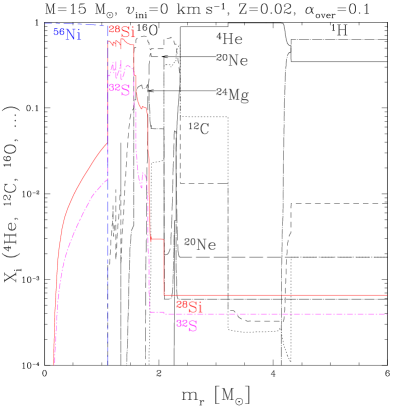
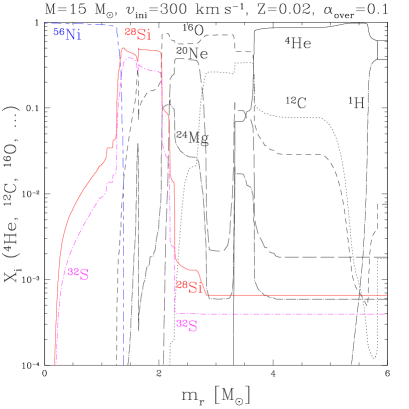
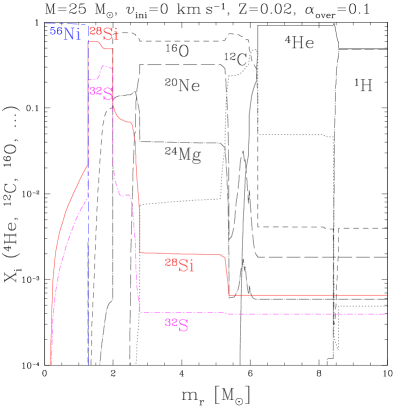
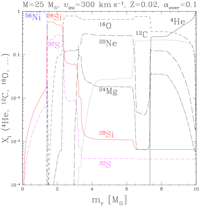
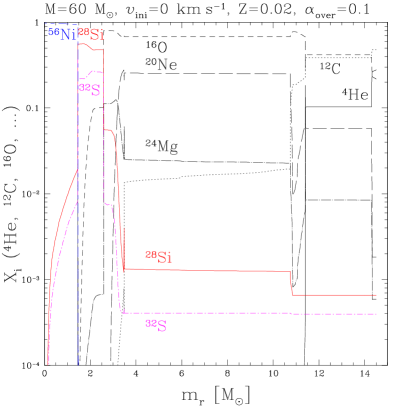
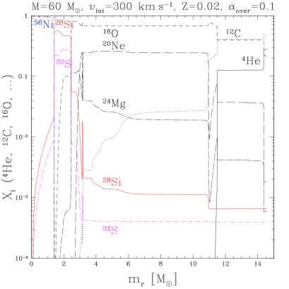
Figure 1: Abundance profile at the end of core silicon burning for the non–rotating (left) and rotating (right) 15 (top), 25 (middle) and 60 (bottom) $M_{\sun}$ models.

5 Pre–SN contribution

Table 4: Initial mass and velocity and pre–SN contribution to the yields ($mp^{\rm{pre-SN}}_{im}$) of solar metallicity models. All masses and yields are in solar mass units and velocities are in km s^-1. ”A” in column 2 means wind anisotropy has been included in the model. Z is the total metal content and is defined by: Z$=1-X_{\rm{{}^{1}H}}-X_{\rm{{}^{3}He}}-X_{\rm{{}^{4}He}}$.

$M_{\rm{ini}}$	$\upsilon_{\rm{ini}}$	3He	4He	12C	13C	14N	16O	17O	18O	Z
12	0	-1.22E-4	1.19E+0	8.74E-2	5.83E-4	3.59E-2	2.07E-1	3.45E-5	1.62E-4	4.57E-1
12	300	-1.45E-4	1.48E+0	1.66E-1	8.72E-4	3.52E-2	3.94E-1	2.68E-5	1.69E-3	7.97E-1
15	0	-1.87E-4	1.67E+0	1.54E-1	5.51E-4	4.23E-2	4.34E-1	1.51E-5	2.76E-3	9.19E-1
15	300	-1.75E-4	1.24E+0	3.68E-1	4.90E-4	2.13E-2	1.02E+0	3.87E-6	3.76E-3	1.92E+0
20	0	-2.88E-4	2.03E+0	2.17E-1	4.39E-4	4.72E-2	1.20E+0	7.76E-6	3.92E-3	2.17E+0
20	300	-1.81E-4	3.47E-1	4.50E-1	-2.09E-4	2.81E-4	2.60E+0	-2.30E-5	-9.54E-5	3.98E+0
25	0	-3.74E-4	2.18E+0	3.74E-1	-2.51E-5	5.76E-2	2.18E+0	-6.73E-6	-1.74E-4	3.74E+0
25	300	-2.04E-4	-8.31E-1	7.62E-1	-2.65E-4	-5.60E-3	3.61E+0	-2.72E-5	4.34E-4	5.75E+0
40	0	-2.90E-4	-1.64E+0	6.94E-1	-4.10E-4	-1.05E-2	6.23E+0	-3.88E-5	-2.20E-4	8.66E+0
40	300A	-2.56E-4	-2.08E+0	1.51E+0	-3.62E-4	-9.31E-3	5.03E+0	-3.43E-5	-1.94E-4	8.28E+0
60	0	-2.98E-4	-2.45E+0	1.42E+0	-4.21E-4	-1.08E-2	6.03E+0	-3.99E-5	-2.26E-4	9.66E+0
60	300A	-2.99E-4	-2.40E+0	1.49E+0	-4.22E-4	-1.09E-2	6.01E+0	-4.00E-5	-2.27E-4	9.63E+0

Table 5: Pre–SN contribution to the yields ($mp^{\rm{pre-SN}}_{im}$) of solar metallicity models. Continuation of Table 4. Note that ²⁰Ne yields are an upper limit and may be reduced by Ne–explosive burning and that ²⁴Mg yields may also be modified by neon and oxygen explosive burnings. See discussion in Sect. 6.3.

$M_{\rm{ini}}$	$\upsilon_{\rm{ini}}$	(20Ne)	22Ne	(24Mg)
12	0	1.05E-1	6.80E-3	6.75E-3
12	300	1.58E-1	1.55E-2	1.36E-2
15	0	1.10E-1	1.60E-2	6.06E-2
15	300	2.26E-1	3.33E-2	4.27E-2
20	0	4.83E-1	3.64E-2	1.28E-1
20	300	6.80E-1	4.26E-2	1.19E-1
25	0	8.41E-1	5.22E-2	1.38E-1
25	300	1.08E+0	2.24E-2	1.48E-1
40	0	1.36E+0	5.58E-3	1.52E-1
40	300A	1.42E+0	6.93E-3	1.20E-1
60	0	1.81E+0	6.58E-3	1.73E-1
60	300A	1.75E+0	7.60E-3	1.44E-1

Table 6: Initial mass and velocity and total stellar yields ($mp^{\rm{pre-SN}}_{im}+mp^{\rm{wind}}_{im}$) of solar metallicity models. All masses and yields are in solar mass units and velocities are in km s^-1. ”A” means wind anisotropy has been included in the model. Z is the total metal content and is defined by: Z$=1-X_{\rm{{}^{1}H}}-X_{\rm{{}^{3}He}}-X_{\rm{{}^{4}He}}$. These are the yields to be used for chemical evolution models using Eq. 2 from (Maeder, 1992).

$M_{\rm{ini}}$	$\upsilon_{\rm{ini}}$	3He	4He	12C	13C	14N	16O	17O	18O	Z
12	0	-1.24E-4	1.20E+0	8.69E-2	6.08E-4	3.68E-2	2.07E-1	3.59E-5	1.60E-4	4.57E-1
12	300	-1.61E-4	1.60E+0	1.63E-1	1.08E-3	4.04E-2	3.92E-1	3.47E-5	1.67E-3	7.97E-1
15	0	-1.91E-4	1.67E+0	1.53E-1	7.05E-4	4.33E-2	4.34E-1	1.60E-5	2.76E-3	9.19E-1
15	300	-2.27E-4	1.57E+0	3.61E-1	1.07E-3	3.52E-2	1.01E+0	2.02E-5	3.72E-3	1.92E+0
20	0	-2.98E-4	2.08E+0	2.16E-1	6.32E-4	4.96E-2	1.20E+0	8.94E-6	3.91E-3	2.17E+0
20	300	-3.36E-4	1.62E+0	4.33E-1	1.01E-3	4.33E-2	2.57E+0	-2.75E-6	-1.96E-4	3.98E+0
25	0	-4.34E-4	2.57E+0	3.68E-1	4.13E-4	7.40E-2	2.17E+0	-3.34E-6	-2.12E-4	3.74E+0
25	300	-4.51E-4	2.14E+0	7.37E-1	9.57E-4	7.38E-2	3.55E+0	-1.69E-5	2.66E-4	5.75E+0
40	0	-7.06E-4	3.01E+0	6.49E-1	3.01E-4	1.35E-1	6.12E+0	-4.98E-5	-5.24E-4	8.65E+0
40	300A	-8.39E-4	5.89E+0	3.11E+0	1.80E-4	1.63E-1	5.36E+0	-7.35E-5	-6.05E-4	1.05E+1
60	0	-1.13E-3	6.96E+0	3.94E+0	-6.23E-6	2.26E-1	6.47E+0	-1.02E-4	-8.58E-4	1.30E+1
60	300A	-1.37E-3	1.28E+1	4.51E+0	-1.11E-4	2.98E-1	6.41E+0	-1.38E-4	-1.04E-3	1.35E+1

As said above, our pre–SN yields, $mp^{\rm{pre-SN}}_{im}$, were calculated at the end of core Si–burning using the remnant mass, $M_{\rm{rem}}$, given in Table 2. We therefore concentrate on yields of light elements which depend mainly on the evolution prior to core Si–burning.

Before discussing the pre–SN yields, it is interesting to look at the abundance profiles at the pre–SN stage presented in Fig. 1 and at the size of helium and carbon-oxygen cores given in Table 2. The core sizes are clearly increased due to rotational mixing. We also see that as the initial mass of the model increases, the core masses get closer and closer to the final mass of the star. $M_{\alpha}$ reaches the final mass of the star when $M_{\rm{ini}}\gtrsim 40\,M_{\odot}$ for non–rotating models and when $M_{\rm{ini}}\gtrsim 25\,M_{\odot}$ for rotating models. $M_{\rm{CO}}$ becomes close to the final mass for both rotating and non–rotating models for $M_{\rm{ini}}\gtrsim 40\,M_{\odot}$.

The pre–SN yields are presented in Tables 4 and 5. One surprising result in Table 4 is the negative pre–SN yields of ⁴He (and of ¹⁴N) for WR stars. This is simply due to the definition of stellar yields, in which the initial composition is deducted from the final one. As said above, $M_{\rm{CO}}$ becomes close to the final mass for $M_{\rm{ini}}\gtrsim 40\,M_{\odot}$. Since the CO core is free of helium, it is then understandable that the pre–SN yields of ⁴He for WR stars is negative.

5.1 Carbon, oxygen and metallic yields

If mixing is dominant ($M\lesssim 30\,M_{\sun}$), the larger the initial mass, the larger the metallic yields (because the various cores become larger). Rotation increases the core sizes by extra mixing and therefore the total metallic yields are larger for rotating models. Overshooting also plays a role in the core sizes. The larger the overshooting parameter, the larger the cores and the larger the yields. If we compare our rotating and non–rotating models, we see that the pre–SN total metallic yields and ¹²C and ¹⁶O yields in particular are enhanced by rotation by a factor 1.5–2.5 below 30 $M_{\sun}$.

For very massive stars ($M\gtrsim 30\,M_{\sun}$), the higher the mass loss, the smaller the final mass and the total metallic yields. The same explanations work well in general for carbon and oxygen.

6 Total stellar yields

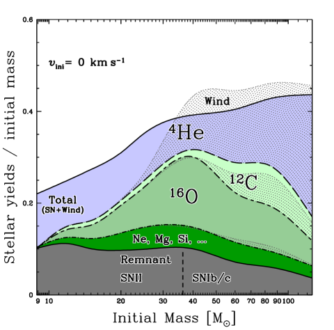
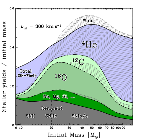
Figure 2: Stellar yields divided by the initial mass, $p^{\rm{tot}}_{im}$, as a function of the initial mass for the non–rotating (left) and rotating (right) models at solar metallicity. The different total yields (divided by $m$) are shown as piled up on top of each other and are not overlapping. ⁴He yields are delimited by the top solid and long dashed lines (top shaded area), ¹²C yields by the long dashed and short–long dashed lines, ¹⁶O yields by the short–long dashed and dotted–dashed lines and the rest of metals by the dotted–dashed and bottom solid lines. The bottom solid line also represents the mass of the remnant ($M^{\rm{int}}_{\rm{rem}}/m$). The corresponding SN explosion type is also given. The wind contributions are superimposed on these total yields for the same elements between their bottom limit and the dotted line above it. Dotted areas help quantify the fraction of the total yields due to winds. Note that for ⁴He, the total yields is smaller than the wind yields due to negative SN yields (see text). Preliminary results for masses equal to 9, 85 and 120 $M_{\odot}$ were used in this diagram (see Hirschi, 2004).

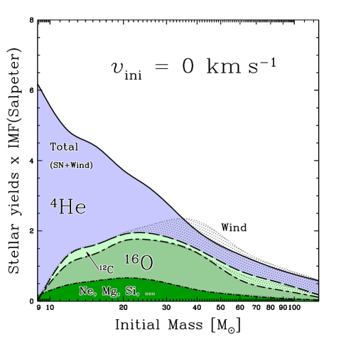
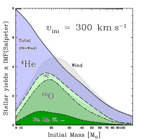
Figure 3: Product of the stellar yields, $mp^{\rm{tot}}_{im}$ by Salpeter’s IMF (multiplied by a arbitrary constant: 1000 x $M^{-2.35}$), as a function of the initial mass for the non–rotating (left) and rotating (right) models at solar metallicity. The different shaded areas correspond from top to bottom to $mp^{\rm{tot}}_{im}$ x 1000 x $M^{-2.35}$ for ⁴He, ¹²C, ¹⁶O and the rest of the heavy elements. The dotted areas show for ⁴He, ¹²C and ¹⁶O the wind contribution. Preliminary results for masses equal to 9, 85 and 120 $M_{\odot}$ were used in this diagram (see Hirschi, 2004).

6.1 Comparison between the wind and pre–SN contributions

The total stellar yields, $mp^{\rm{tot}}_{im}=mp^{\rm{pre-SN}}_{im}+mp^{\rm{wind}}_{im}$ (to be used for chemical evolution models using Eq. 2 from Maeder, 1992), are presented in Tables 6 and 7. What is the relative importance of the wind and pre–SN contributions? Figure 2 displays the total stellar yields divided by the initial mass of the star, $p^{\rm{tot}}_{im}$, as a function of its initial mass, $m$, for the non–rotating (left) and rotating (right) models. The different shaded areas correspond from top to bottom to $p^{\rm{tot}}_{im}$ for ⁴He, ¹²C, ¹⁶O and the rest of the heavy elements. The fraction of the star locked in the remnant as well as the expected explosion type are shown at the bottom. The dotted areas show the wind contribution for ⁴He, ¹²C and ¹⁶O.

For ⁴He (and other H–burning products like ¹⁴N), the wind contribution increases with mass and dominates for $M\gtrsim 22M_{\sun}$ for rotating stars and $M\gtrsim 35M_{\sun}$ for non–rotating stars, i. e. for the stars which enter the WR stage. As said earlier, for very massive stars, the SN contribution is negative and this is why $p^{\rm{tot}}_{{}^{4}\rm{He}m}$ is smaller than $p^{\rm{wind}}_{{}^{4}\rm{He}m}$. In order to eject He–burning products, a star must not only become a WR star but must also become a WC star. Therefore for ¹²C, the wind contributions only start to be significant above the following approximative mass limits: 30 and 45 $M_{\sun}$ for rotating and non–rotating models respectively. Above these mass limits, the contribution from the wind and the pre–SN are of similar importance. Since at solar metallicity, no WO star is produced (Meynet & Maeder, 2004), for ¹⁶O, as for heavier elements, the wind contribution remains very small.

6.2 Comparison between rotating and non–rotating models

For H–burning products, the yields of the rotating models are usually higher than those of non–rotating models. This is due to larger cores and larger mass loss. Nevertheless, between about 15 and 25 $M_{\sun}$, the rotating yields are smaller. This is due to the fact that the winds do not expel many H–burning products yet and more of these products are burnt later in the pre–supernova evolution (giving negative SN yields). Above 40 $M_{\sun}$, rotation clearly increases the yields of ⁴He.

Concerning He–burning products, below 30 $M_{\sun}$, most of the ¹²C comes for the pre–SN contribution. In this mass range, rotating models having larger cores also have larger yields (factor 1.5–2.5). We notice a similar dependence on the initial mass for the yields of non–rotating models as for the yields of rotating models, but shifted to higher masses. Above 30 $M_{\sun}$, where mass loss dominates, the yields from the rotating models are closer to those of the non–rotating models. The situation for ¹⁶O and metallic yields is similar to carbon. Therefore ¹²C, ¹⁶O and the total metallic yields are larger for our rotating models compared to our non–rotating ones by a factor 1.5–2.5 below 30 ${\mathbf{M}_{\odot}}$.

Figure 3 presents the stellar yields convolved with the Salpeter initial mass function (IMF) ($dN/dM\propto M^{-2.35}$). This reduces the importance of the very massive stars. Nevertheless, the differences between rotating and non–rotating models remain significant, especially around $20\,M_{\odot}$.

Table 7: Total stellar yields ($mp^{\rm{pre-SN}}_{im}+mp^{\rm{wind}}_{im}$) of solar metallicity models. Continuation of Table 6. Note that ²⁰Ne yields are an upper limit and may be reduced by Ne–explosive burning and that ²⁴Mg yields can also be modified by neon and oxygen explosive burnings. See discussion in Sect. 6.3.

$M_{\rm{ini}}$	$\upsilon_{\rm{ini}}$	(20Ne)	22Ne	(24Mg)
12	0	1.05E-1	6.80E-3	6.75E-3
12	300	1.58E-1	1.55E-2	1.36E-2
15	0	1.10E-1	1.60E-2	6.06E-2
15	300	2.26E-1	3.33E-2	4.27E-2
20	0	4.83E-1	3.64E-2	1.28E-1
20	300	6.80E-1	4.26E-2	1.19E-1
25	0	8.41E-1	5.22E-2	1.38E-1
25	300	1.08E+0	2.26E-2	1.48E-1
40	0	1.36E+0	5.58E-3	1.52E-1
40	300A	1.42E+0	8.05E-2	1.20E-1
60	0	1.81E+0	1.35E-1	1.73E-1
60	300A	1.75E+0	1.74E-1	1.44E-1

6.3 Comparison with the literature

Figure 4: Left: total ejected masses (EM) of ¹H, ⁴He, ¹²C and ¹⁶O as a function of the initial mass for different non–rotating models at solar metallicity. Right: total ejected masses (EM) of ¹⁶O, ²⁰Ne and ²⁴Mg as a function of the CO core mass for different models at solar metallicity. Solid lines (HMM04) represent our results, dotted lines (LC03) show the results from Limongi & Chieffi (2003), long–short dashed lines (TNH96) show the results from Thielemann et al. (1996), dashed lines (RHW02) represent the results from Rauscher et al. (2002) and dotted–dashed (WW95) lines show the results from Woosley & Weaver (1995).

Table 8: Initial mass and velocity, remnant mass and total ejected masses (EM) of solar metallicity models. All masses are in solar mass units and velocities are in km s^-1. ”A” in column 2 means wind anisotropy has been included in the model. Note that this table is given for comparison with other recent publications and does not correspond to our definition of yields (see Sect. 3).

$M_{\rm{ini}}$	$\upsilon_{\rm{ini}}$	$M_{\rm{rem}}$	1H	3He	4He	12C	13C	14N	16O	17O	18O	Z
12	0	1.34	5.86E+0	1.87E-4	4.13E+0	1.23E-1	1.05E-3	4.81E-2	3.09E-1	7.75E-5	3.95E-4	6.70E-1
12	300	1.46	5.03E+0	1.46E-4	4.50E+0	1.99E-1	1.51E-3	5.16E-2	4.93E-1	7.58E-5	1.91E-3	1.01E+0
15	0	1.51	6.92E+0	2.02E-4	5.38E+0	1.99E-1	1.26E-3	5.76E-2	5.64E-1	6.86E-5	3.06E-3	1.19E+0
15	300	1.85	5.78E+0	1.56E-4	5.19E+0	4.06E-1	1.61E-3	4.91E-2	1.14E+0	7.14E-5	4.01E-3	2.18E+0
20	0	1.95	8.48E+0	2.28E-4	7.05E+0	2.77E-1	1.38E-3	6.88E-2	1.37E+0	7.94E-5	4.31E-3	2.53E+0
20	300	2.57	6.69E+0	1.72E-4	6.41E+0	4.93E-1	1.73E-3	6.17E-2	2.74E+0	6.52E-5	1.89E-4	4.33E+0
25	0	2.49	9.57E+0	2.22E-4	8.76E+0	4.45E-1	1.34E-3	9.79E-2	2.39E+0	8.45E-5	2.85E-4	4.19E+0
25	300	3.06	7.57E+0	1.89E-4	8.18E+0	8.12E-1	1.86E-3	9.70E-2	3.76E+0	6.87E-5	7.51E-4	6.19E+0
40	0	4.02	1.36E+1	3.40E-4	1.29E+1	7.72E-1	1.78E-3	1.73E-1	6.47E+0	9.01E-5	2.69E-4	9.37E+0
40	300A	3.85	9.11E+0	2.14E-4	1.58E+1	3.24E+0	1.67E-3	2.02E-1	5.71E+0	6.73E-5	1.93E-4	1.12E+1
60	0	4.30	1.91E+1	4.85E-4	2.22E+1	4.13E+0	2.28E-3	2.84E-1	7.01E+0	1.14E-4	3.68E-4	1.41E+1
60	300A	4.32	1.29E+1	2.56E-4	2.81E+1	4.70E+0	2.18E-3	3.57E-1	6.94E+0	7.86E-5	1.94E-4	1.46E+1

We compare here the yields of the non–rotating models with other authors. For this purpose, the ejected masses, $EM$, defined by Eq. 4 in Sect. 3, are presented in Tables 8 and 9. Figure 4 shows the comparison with four other calculations: Limongi & Chieffi (2003) (LC03), Thielemann et al. (1996) (TNH96), Rauscher et al. (2002) (RHW02) and Woosley & Weaver (1995) (WW95). For LC03, we chose the remnant masses that are closest to ours (models 15D, 20B, 25A). The uncertainties related to convection and the ¹²C$(\alpha,\gamma)^{16}$O reaction are dominant. Therefore, before we compare our results with other models, we briefly mention here which treatment of convection and ¹²C$(\alpha,\gamma)^{16}$O rate other authors use:

• Limongi & Chieffi (2003) use Schwarzschild criterion (except for the H convective shell that forms at the end of core H–burning, where Ledoux criterion is used) for convection without overshooting. For ¹²C$(\alpha,\gamma)^{16}$O, they use the rate of Kunz et al. (2002) (K02).

• Thielemann et al. (1996) use Schwarzschild criterion for convection without overshooting. For ¹²C$(\alpha,\gamma)^{16}$O, they use the rate of Caughlan et al. (1985) (CF85).

• Woosley & Weaver (1995) use Ledoux criterion for convection with semiconvection. They use a relatively large diffusion coefficient to model semiconvection. Moreover non–convective zones immediately adjacent to convective regions are slowly mixed over the order of a radiation diffusion time scale to approximately allow for the effects of convective overshoot. For ¹²C$(\alpha,\gamma)^{16}$O, they use the rate of Caughlan & Fowler (1988) (CF88) multiplied by 1.7.

• Rauscher et al. (2002) use Ledoux criterion for convection with semiconvection. They use the same method as WW95 for semiconvection. For ¹²C$(\alpha,\gamma)^{16}$O, they use the rate of Buchmann (1996) (BU96) multiplied by 1.2.

• In this paper (HMM04), we use Schwarzschild criterion for convection with overshooting. For ¹²C$(\alpha,\gamma)^{16}$O, we use the rate of Angulo et al. (1999) (NACRE).

A comparison of the different reaction rates and treatment of convection is presented in Hirschi et al. (2004). The comparison of the ejected masses is shown in Fig. 4 for masses between 15 and 25 $M_{\odot}$. The ⁴He and ¹⁶O yields are larger when respectively the helium and carbon–oxygen cores are larger. This can be seen by comparing our models with those of RHW02 and LC03 (Fig. 4 and respective tables of core masses).

For ¹²C yields, the situation is more complex because the larger the cores, the larger the central temperature and the more efficient the ¹²C$(\alpha,\gamma)^{16}$O reaction. If we only consider the effect of this reaction we have that the larger the rate, the smaller the ¹²C abundance at the end of He–burning and the smaller the corresponding yield (and the larger the ¹⁶O yield). This can be seen in Fig. 4 by comparing our ¹²C and ¹⁶O yields with those of LC03 (we both use Schwarzschild criterion). Indeed the NACRE rate is larger than the K02 one so our ¹²C yield is smaller. THN96 (who also use Schwarzschild criterion) using the rate of Caughlan et al. (1985) which is even larger, obtain an even smaller ¹²C yield. When both the convection treatment and the ¹²C$(\alpha,\gamma)^{16}$O rate are different, the comparison becomes more complicated. Nevertheless, within the model uncertainties, the yields of various models agree. In fact, the uncertainties are reduced when we use the CO core mass instead of the initial mass in order to compare the results of different groups. Fig. 4 (right) shows the small uncertainty for ¹⁶O in relation to the CO core mass. This confirms the relation $M_{\rm{CO}}$–yields(¹⁶O) and shows that this relation holds for models of different groups and for models of non–rotating and rotating stars.

We calculated the pre–SN yields at the end of Si–burning. Therefore, the yields of ²⁰Ne and ²⁴Mg may still be affected by explosive neon and oxygen burnings. ²⁰Ne yields are upper limits due to the possible destruction of this element by explosive Ne–burning. Figure 4 (right) shows that our results lies above the results of other groups but that the difference is as small as differences between the results of the other groups. ²⁴Mg yields are also close to the results of other groups who included explosive burnings in their calculations. By comparing our results for ²⁰Ne and ²⁴Mg with the other groups mentioned above, we see that the difference between our results and the results of other groups is as small as the differences between the 19, 20 and 21 $M_{\odot}$ models of Rauscher et al. (2002) and differences between for example Rauscher et al. (2002) and Limongi & Chieffi (2003). This means that our yields for these two elements are good approximations even though explosive burning was not followed in this calculation. For ²⁴Mg, it is interesting to note that rotation increases significantly the yields only for the 12 $M_{\odot}$ models and that, in general, rotation slightly decreases the ²⁴Mg yields in the massive star range (see Table 7 and Fig. 4 right). This point is interesting for chemical evolution of galaxies since it goes in the same direction as observational constraints (François et al., 2004).

For ¹⁷O yields, all recent calculations agree rather well and differ from the WW95 results because of the change in the reaction rates (especially ¹⁷O$(p,\alpha)^{14}$N, see Aubert et al., 1996). ¹⁸O and ²²Ne are produced by $\alpha$–captures on ¹⁴N. As said in Sect. 3, ²²Ne is not followed during the advanced stages and we had to use a special calculation for its yield. Our ²²Ne values are nevertheless very close to other calculations (see Hirschi, 2004).

Table 9: Total ejected masses (EM) of solar metallicity models. Continuation of Table 8.

$M_{\rm{ini}}$	$\upsilon_{\rm{ini}}$	(20Ne)	22Ne	(24Mg)
12	0	1.24E-1	8.37E-3	1.27E-2
12	300	1.77E-1	1.71E-2	1.87E-2
15	0	1.35E-1	1.80E-2	6.75E-2
15	300	2.50E-1	3.53E-2	4.77E-2
20	0	5.16E-1	3.90E-2	1.36E-1
20	300	7.12E-1	4.52E-2	1.23E-1
25	0	8.82E-1	5.55E-2	1.45E-1
25	300	1.12E+0	2.59E-2	1.52E-1
40	0	1.42E+0	1.08E-2	1.58E-1
40	300A	1.48E+0	8.58E-2	1.25E-1
60	0	1.91E+0	1.43E-1	1.79E-1
60	300A	1.86E+0	1.82E-1	1.50E-1

7 Conclusion

We calculated a new set of stellar yields of rotating stars at solar metallicity covering the massive star range (12–60 $M_{\sun}$). We used for this purpose the latest version of the Geneva stellar evolution code described in Hirschi et al. (2004). We present the separate contribution to stellar yields by winds and supernova explosion. For the wind contribution, our rotating models have larger yields than the non–rotating ones because of the extra mass loss and mixing due to rotation. For the SN yields, we followed the evolution and nucleosynthesis until core silicon burning. Since we did not model the SN explosion and explosive nucleosynthesis, we present pre–SN yields for elements lighter than ²⁸Si, which depend mostly on the evolution prior to Si–burning. Our results for the non–rotating models correspond very well to other calculations and differences can be understood in the light of the treatment of convection and the rate used for ¹²C$(\alpha,\gamma)^{16}$O. This assesses the accuracy of our calculations and assures a safe basis for the yields of our rotating models.

For the pre–SN yields and for masses below $\sim 30\,M_{\sun}$, rotating models have larger yields. The ¹²C and ¹⁶O yields are increased by a factor of 1.5–2.5 by rotation in the present calculation. When we add the two contributions, the yields of most heavy elements are larger for rotating models below $\sim 30\,M_{\sun}$. Rotation increases the total metallic yields by a factor of 1.5–2.5. As a rule of thumb, the yields of a rotating 20 $M_{\odot}$ star are similar to the yields of a non–rotating 30 $M_{\odot}$ star, at least for the light elements considered in this work. When mass loss is dominant (above $\sim 30\,M_{\sun}$) our rotating and non–rotating models give similar yields for heavy elements. Only the yields of H–burning products are increased by rotation in the very massive star range.

References

- Anders & Grevesse (1989) Anders, E. & Grevesse, N. 1989, Geochim. Cosmochim. Acta., 53, 197
- Angulo et al. (1999) Angulo, C., Arnould, M., Rayet, M., et al. 1999, Nuclear Physics A, 656, 3
- Aubert et al. (1996) Aubert, O., Prantzos, N., & Baraffe, I. 1996, A&A, 312, 845
- Buchmann (1996) Buchmann, L. 1996, ApJ, 468, L127
- Caughlan & Fowler (1988) Caughlan, G. R. & Fowler, W. A. 1988, Atomic Data and Nuclear Data Tables, 40, 283
- Caughlan et al. (1985) Caughlan, G. R., Fowler, W. A., Harris, M. J., & Zimmerman, B. A. 1985, Atomic Data and Nuclear Data Tables, 32, 197
- Chieffi & Limongi (2003) Chieffi, A. & Limongi, M. 2003, PASA, 20, 324
- de Jager et al. (1988) de Jager, C., Nieuwenhuijzen, H., & van der Hucht, K. A. 1988, A&AS, 72, 259
- François et al. (2004) François, P., Matteucci, F., Cayrel, R., et al. 2004, A&A, 421, 613
- Fukuda (1982) Fukuda, I. 1982, PASP, 94, 271
- Hirschi (2004) Hirschi, R. 2004, Ph.D. Thesis, http://quasar.physik.unibas.ch/ hirschi/workd/thesis.pdf
- Hirschi et al. (2004) Hirschi, R., Meynet, G., & Maeder, A. 2004, A&A, 425, 649
- Janka et al. (2004) Janka, H. ., Buras, R., Joyanes, F. S. K., et al. 2004, astro–ph0411347, contribution to NIC8
- Janka et al. (2003) Janka, H.-T., Buras, R., Kifonidis, K., Plewa, T., & Rampp, M. 2003, in From Twilight to Highlight: The Physics of Supernovae, 39
- Kunz et al. (2002) Kunz, R., Fey, M., Jaeger, M., et al. 2002, ApJ, 567, 643
- Langer (1989) Langer, N. 1989, A&A, 220, 135
- Limongi & Chieffi (2003) Limongi, M. & Chieffi, A. 2003, ApJ, 592, 404
- Maeda & Nomoto (2003) Maeda, K. & Nomoto, K. 2003, ApJ, 598, 1163
- Maeder (1992) Maeder, A. 1992, A&A, 264, 105
- Maeder & Meynet (2000a) Maeder, A. & Meynet, G. 2000a, A&A, 361, 159
- Maeder & Meynet (2000b) —. 2000b, ARA&A, 38, 143
- Maeder & Meynet (2001) —. 2001, A&A, 373, 555
- Meynet & Maeder (2002) Meynet, G. & Maeder, A. 2002, A&A, 381, L25
- Meynet & Maeder (2003) —. 2003, A&A, 404, 975
- Meynet & Maeder (2004) —. 2004, A&A, in press
- Meynet et al. (1994) Meynet, G., Maeder, A., Schaller, G., Schaerer, D., & Charbonnel, C. 1994, A&AS, 103, 97
- Nugis & Lamers (2000) Nugis, T. & Lamers, H. J. G. L. M. 2000, A&A, 360, 227
- Rauscher et al. (2002) Rauscher, T., Heger, A., Hoffman, R. D., & Woosley, S. E. 2002, ApJ, 576, 323
- Thielemann et al. (1996) Thielemann, F., Nomoto, K., & Hashimoto, M. 1996, ApJ, 460, 408
- Travaglio et al. (2004) Travaglio, C., Kifonidis, K., & Müller, E. 2004, New Astronomy Review, 48, 25
- Vink et al. (2000) Vink, J. S., de Koter, A., & Lamers, H. J. G. L. M. 2000, A&A, 362, 295
- Vink et al. (2001) —. 2001, A&A, 369, 574
- Woosley et al. (1995) Woosley, S. E., Langer, N., & Weaver, T. A. 1995, ApJ, 448, 315
- Woosley & Weaver (1995) Woosley, S. E. & Weaver, T. A. 1995, ApJS, 101, 181