ESTIMATING THE GALAXY CORRELATION LENGTH $r_{0}$ FROM THE NUMBER OF GALAXY PAIRS WITH SIMILAR REDSHIFTS

Abstract

We discuss methods that can be used to estimate the spatial correlation length $r_{0}$ of galaxy samples from the observed number of pairs with similar redshifts. The standard method is unnecessarily noisy and can be compromised by errors in the assumed selection function. We present three alternatives, one less noisy, one that responds differently to systematic errors, the third insensitive to the selection function, and quantify their performance by applying them to a cosmological N-body simulation and to the Lyman-break survey of galaxies at redshift $z\sim 3$. Researchers adopting the standard method could easily conclude that the Lyman-break galaxy comoving correlation length was $r_{0}\sim 11h^{-1}$ Mpc, several times larger than the correct value. The use of our proposed methods would make this error impossible, except in the small sample limit. When $N_{\rm gal}\lower 2.15277pt\hbox{$\;\buildrel<\over{\sim}\;$}20$, major errors in estimates of $r_{0}$ occur alarmingly often.

1 INTRODUCTION

This paper was inspired by the work of Daddi et al. (2002, 2004), Blain et al. (2004), and others who have estimated the spatial clustering strength of a galaxy population from the observed positions of a small number of its members. Unable to fit a correlation function to the binned numbers of pair counts at different spatial separations, these authors counted the number $n_{\rm obs}$ of galaxy pairs with redshift separation $|z_{1}-z_{2}|<\Delta z$ and compared to the expected number $n_{\rm exp}$ for an assumed correlation function $\xi(r)$, which Blain et al. (2004) calculated to be

$$n_{\rm exp}=\frac{N^{2}}{2\Omega^{2}}\int_{0}^{\infty}dz_{1}P(z_{1})\int_{z_{1}-\Delta z}^{z_{1}+\Delta z}dz_{2}P(z_{2})\int_{\Omega}d{\bf\Theta_{1}}\int_{\Omega}d{\bf\Theta_{2}}[1+\xi(r_{12})],$$ (1)

where $N$ is the number of galaxies with measured redshifts, $P(z)$ is the survey selection function, $\Omega$ is the solid angle of the survey, $r_{12}$ is the comoving distance between the points specified by $({\bf\Theta_{1}},z_{1})$ and $({\bf\Theta_{2}},z_{2})$, and ${\bf\Theta}$ is the angular position of a galaxy within $\Omega$. They then restricted their attention to a family of correlation functions $\xi(r)=(r/r_{0})^{-1.8}$ that could be specified by a single parameter, $r_{0}$, and estimated $r_{0}$ for their galaxy population by finding the value that made $n_{\rm exp}=n_{\rm obs}$. Inspired by Poisson statistics, Blain et al. (2004) took as a $1\sigma$ confidence interval the set of $r_{0}$ that satisfied

$$n_{\rm obs}-n_{\rm obs}^{1/2}<n_{\rm exp}(r_{0})<n_{\rm obs}+n_{\rm obs}^{1/2}.$$ (2)

The approach can provide useful constraints on $r_{0}$ when other methods fail, but the implementation described above is imperfect. Equation 1 is unnecessarily noisy and is more sensitive to the assumed selection function than to the clustering strength $\bar{\xi}$; equation 2 almost always underestimates the true uncertainty in $r_{0}$. The goal of this paper is to draw attention to these shortcomings and to suggest modifications that make the analysis less subject to them. Section 3.1 discusses the effect of uncertainties in the selection function, showing that a 20% error in the assumed width of a Gaussian selection function can easily change the inferred value of $r_{0}$ by a factor of 2 or more. Sections 3.2 and 3.3 point out two additional sources of noise in equation 1 that are easily removed. My suggested revisions to the method are put forward in § 4 and tested with a cosmological $N$-body simulation in § 5. Section 6 considers the uncertainty in the best-fit values of $r_{0}$, showing that equation 2 is a poor approximation and suggesting a modification that leads to more realistic error bars. The main conclusions are summarized and discussed in § 7. To motivate the discussion, I begin in § 2 with an example that shows the standard analysis of redshift pair-counts going badly awry.

2 A FAULTY ANALYSIS OF LYMAN-BREAK GALAXIES

The analyzed sample consists of the 747 Lyman-break galaxies with apparent magnitude $23.5<{\cal R}<25.5$ in the fields 3c324, b20902, CDFa, CDFb, DSF2237a, DSF2237b, HDF, Q0201, Q0256, Q0302, Q0933, Q1422, SSA22a, SSA22b, and Westphal whose spectroscopic redshifts were published by Steidel et al. (2003). The size of the observed fields varied but was typically $9^{\prime}\times 9^{\prime}$. I calculated the observed number of pairs with comoving radial separation $Z<20h^{-1}$ Mpc in each field individually. Summing over all fields, a total of $n_{\rm obs}=2539$ pairs were found with comoving radial separations in this range. Since the Lyman-break technique selects galaxies over a broad range of redshifts $2.3\lower 2.15277pt\hbox{$\;\buildrel<\over{\sim}\;$}z\lower 2.15277pt\hbox{$\;\buildrel<\over{\sim}\;$}3.7$, I approximated the selection function $P(z)$ as a Gaussian with mean redshift $\mu=3.0$ and standard deviation $\sigma_{\rm sel}=0.4$. To calculate the expected number of pairs with $Z<20h^{-1}$ Mpc in the $i$th field for a given value of $r_{0}$, I inserted this selection function into equation 1, assumed a correlation function slope of $\gamma=1.6$, and integrated numerically over the field’s solid angle $\Omega$. I set the expected total number of pairs $n_{\rm exp}(r_{0})$ equal to the sum of the expected number for each individual field. A value of $r_{0}=11.08h^{-1}$ Mpc was required for $n_{\rm exp}$ to equal $n_{\rm obs}$, while $r_{0}=10.82h^{-1}$ Mpc made $n_{\rm exp}=n_{\rm obs}-n^{1/2}_{\rm obs}$ and $r_{0}=11.33h^{-1}$ Mpc made $n_{\rm exp}=n_{\rm obs}+n^{1/2}_{\rm obs}$. I conclude that the correlation length for Lyman-break galaxies is $r_{0}=11.1\pm 0.25h^{-1}$ Mpc at the $1\sigma$ level.

As noted in the abstract, this estimate of $r_{0}$ is roughly 20$\sigma$ away from the value of $r_{0}\simeq 4.0\pm 0.6h^{-1}$ Mpc measured by Adelberger et al. (2004). What went wrong?

3 SOURCES OF ERROR

3.1 Selection-function Uncertainties

Most of the error in the previous section’s estimate of $r_{0}$ came from the inaccurate model of the redshift selection function. Although it is not always acknowledged in analyses of this sort, assumptions about the selection function have a critical effect on the results. Figure 1 shows that in the example of § 2 the best-fit value of $r_{0}$ changes by more than an order of magnitude as the assumed width of the Gaussian selection function increases from $\sigma_{\rm sel}=0.2$ to $\sigma_{\rm sel}=0.5$. If we had adopted the correct width $\sigma_{\rm sel}=0.3$ (Adelberger et al. 2004) instead of $\sigma_{\rm sel}=0.4$, we would have found $r_{0}=7.2$ instead of $r_{0}=11.1h^{-1}$ Mpc—significantly closer to the true value $r_{0}\sim 4h^{-1}$ Mpc.

Unfortunately analyses similar to the one in § 2 are usually attempted when the sample size is extremely small, too small for $\sigma_{\rm sel}$ to be determined empirically. In this case it is difficult to know which to adopt among the possible values of $r_{0}$ suggested by plots similar to Figure 1. Although theoretical arguments may provide a reasonable estimate of the selection-function shape, it seems sensible to reduce as far as possible the dependence of the answer on the assumed shape.

Approximating the selection function as a boxcar with half-width $L$, equation 1 can be rewritten

$$n_{\rm exp}\propto\frac{C}{L}\biggl{[}1+\bar{\xi}\biggr{]}$$ (3)

where $C$ is an uninteresting constant and $\bar{\xi}$ is the spatially-averaged correlation function defined by equation 1. This form makes it easy to see why the implied value of $r_{0}$ can be so strongly affected by the assumed selection function. If the field size $\Omega$ or redshift separation $\Delta z$ is large compared to $r_{0}$, as is usually the case, $\bar{\xi}$ will be significantly less than unity. The change in $n_{\rm exp}$ that accompanies a significant change in the correlation strength, $|dn_{\rm exp}/d{\rm ln}\bar{\xi}|=C\bar{\xi}/L$, will therefore be considerably smaller than the change in $n_{\rm exp}$ that accompanies significant changes in $L$, $|dn_{\rm exp}/d{\rm ln}L|=C(1+\bar{\xi})/L$, and minor errors in the assumed selection function will lead to major errors in the inferred value of $r_{0}$. Although these results were derived for a boxcar selection function, similar results hold for other types.

One way to reduce the method’s sensitivity to the selection function is to design the experiment to maximize $\bar{\xi}$. Since $\bar{\xi}$ increases as $\Omega$ decreases, experiments with smaller fields-of-view are less affected by uncertainties in the selection function. In practice, however, the field-of-view is set by the instrument that is used and observers are unlikely to want to discard much of their data. Decreasing $\Delta z$ is a more palatable option, but, owing to peculiar velocities and to uncertainties in galaxies’ measured redshifts, it cannot be decreased arbitrarily far before genuine pairs begin to be missed. $10h^{-1}$ comoving Mpc is a rough lower limit for most surveys. Unfortunately this limit is large enough to ensure $\bar{\xi}\lower 2.15277pt\hbox{$\;\buildrel<\over{\sim}\;$}1$ for likely fields-of-view.

Another way is to use the statistic $K$ (Adelberger et al. 2004) instead of $n_{\rm obs}$ in the analysis. This adds noise but removes the sensitivity to the selection function almost completely. The approach is described in more detail below (§§ 4 and 5).

3.2 Angular distribution of sources

An additional shortcoming of equation 1 is its assumption that the sources with measured redshifts have unknown angular positions that are distributed uniformly across the observed region $\Omega$ (see § A.3). In fact the angular positions are known (how else were redshifts measured?) and are probably not uniformly distributed. Consider, for example, a situation where we obtained images across a region with radius $r=20^{\prime}$, but were able to measure redshifts for only 2 galaxies. If these galaxies happened to have an angular separation of $4^{\prime\prime}$, they would be likely to lie at nearly the same redshift even if $r_{0}$ were small, while if they had a separation of $40^{\prime}$ they would be unlikely to lie at the same redshift even if $r_{0}$ were large (Figure 2). Since the expected number of close redshift pairs for a known correlation length $r_{0}$ depends on the galaxies’ angular separations, our attempts to infer $r_{0}$ from the number of pairs will be improved if we take the galaxies’ actual separations into account. Neglecting this information adds noise to the analysis and can bias the results if the spectroscopically observed galaxies were not chosen at random.

3.3 Redshift distribution of sources

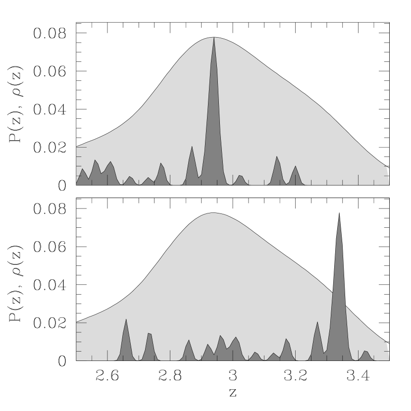
Figure 3: Dependence of the number of redshift pairs on the locations of galaxy overdensities. The lighter shaded region in the background of both panels shows the Lyman-break galaxy selection function $P(z)$. The darker shaded region shows the galaxy density $\rho(z)$ observed in the field SSA22a, shifted by $\Delta z=-0.15$ in the top panel and by $\Delta z=0.25$ in the bottom. The units on the $y$-axis are arbitrary. The galaxy clustering strength is the same in both panels, but the upper panel will have roughly $3.5$ times as many pairs with small redshift separations, on average, since the galaxy overdensity is aligned with the peak of the redshift histogram and since the number of pairs is proportional to $\rho^{2}$. Estimates of $r_{0}$ derived solely from the number of pairs can be led astray by chance alignments or misalignments of galaxy overdensities with the selection function. Section 4 shows how to remove this unnecessary source of noise; see the discussion near equation 5.

Figure 3 illustrates another source of noise. Suppose we have found a single galaxy at redshift $z_{2}$. How many other galaxies should we expect to find in the redshift interval $z_{2}-\Delta z<z<z_{2}+\Delta z$ for an assumed value of $r_{0}$? The answer depends on the distance between $z_{2}$ and the peak of the selection function. If $z_{2}$ lies near the peak, we would expect a large number of pairs even if $r_{0}$ were small; if $z_{2}$ lies in the wings we would expect few pairs even if $r_{0}$ were large. Since the galaxies in pencil beam surveys tend to lie in a small number of prominent spikes in the redshift histogram, the expected number of redshift pairs is strongly affected by the alignment or misalignment of the spikes with the peak of the selection function. Equation 1 is noisier than it needs to be because it ignores the locations of redshift spikes when calculating $n_{\rm exp}$.

4 ALTERNATIVES

This section suggests alternate approaches that are less affected by the shortcomings discussed above. The first two are refinements in the calculation of $n_{\rm exp}$; the last relies on a slightly different statistic. The notation we use is explained more fully in the appendix.

As shown in the appendix, equation 1 (in its correctly normalized form, equation A16) gives the number of redshift pairs one should expect to observe given only the information that $N$ galaxies lie somewhere in the field of view $\Omega$. But what if we know angular positions of the sources? How does this change $n_{\rm exp}$? If $P(|Z_{ij}|<\ell\,|\,\theta_{ij})$ is the probability that a galaxy pair with angular separation $\theta_{ij}$ has comoving radial separation $|Z_{ij}|<\ell$, then the expected total number of redshift-pairs should be equal to the sum over all pairs of $P(|Z_{ij}|<\ell\,|\,\theta_{ij})$:

$$n_{\rm exp}=\sum_{i>j}^{\rm pairs}P(|Z_{ij}|<\ell\,|\,\theta_{ij}).$$ (4)

This equation can be evaluated with the help of equation A11. Using it in place of equation 1 will remove the noise and bias that arises from the angular positions of the sources. The estimated correlation length of Lyman-break galaxies in our example analysis (§ 2), reduced from $11.1h^{-1}$ Mpc to $7.2h^{-1}$ Mpc by the adoption of the correct selection function, is further reduced to $6.4h^{-1}$ Mpc when equation 4 is used instead of equation 1. The reduction from $7.2h^{-1}$ to $6.4h^{-1}$ Mpc results partly from the fact the angular positions of galaxies with measured redshifts were clumped together into slitmask-sized regions, not distributed randomly across the field.

How can we incorporate knowledge of the spike redshifts into the analysis? Suppose we know that one member of a galaxy pair with angular separation $\theta_{ij}$ has the redshift $z_{j}$. Then the probability $P(|Z_{ij}|<\ell\,|\,z_{j}\theta_{ij})$ that the galaxies have radial separation $|Z_{ij}|<\ell$ is given by equation A6. The expected total number of pairs in the sample with redshift separation less than $\ell$ should therefore be equal to the sum of the probabilities for each unique pair,

$$n_{\rm exp}=\frac{1}{2}\sum_{i\neq j}^{\rm pairs}P(|Z_{ij}|<\ell\,|\,z_{j}\theta_{ij}).$$ (5)

Using equation 5 instead of equation 4 further reduces the estimated correlation length (in the example of § 2) to $r_{0}=5.7h^{-1}$ Mpc.

Equations 4 and 5 are as sensitive to errors in the selection function as equation 1. This sensitivity can be eliminated almost completely by using the $K$ statistic of Adelberger et al. (2004) rather than $n_{\rm obs}$ in the analysis. Letting $n_{\rm obs}(0,\ell)$ stand for the observed number of pairs with comoving radial separation $0\leq|Z_{ij}|<\ell$, $K$ is the ratio

$$K\equiv\frac{n_{\rm obs}(0,\ell)}{n_{\rm obs}(0,2\ell)}.$$ (6)

As long as $n_{\rm obs}(0,2\ell)$ is large enough that

$$\Biggl{\langle}\frac{n_{\rm obs}(0,\ell)}{n_{\rm obs}(0,2\ell)}\Biggr{\rangle}\simeq\frac{\langle n_{\rm obs}(0,\ell)\rangle}{\langle n_{\rm obs}(0,2\ell)\rangle},$$ (7)

$K$ will have expectation value

$$\langle K\rangle\simeq\frac{n_{\rm exp}(0,\ell)}{n_{\rm exp}(0,2\ell)}.$$ (8)

(In this equation, $n_{\rm exp}(0,\ell)$ can be calculated with equation 4, equation 5, or any number of variants; the value of $K$ will not change significantly.) Adelberger et al. (2004) show that the right-hand size of equation 8 is almost entirely independent of the assumed selection-function width $\sigma_{\rm sel}$ when $2\ell$ is small compared to $\sigma_{\rm sel}$. If we find the value of $r_{0}$ that makes the right-hand side of equation 8 equal the right-hand side of equation 6, we will have an estimate of the correlation length whose value does not depend on our assumptions about the selection function. This is our final approach to estimating $r_{0}$. Applying it to the Lyman-break galaxy example of § 2 leads to an estimate $r_{0}=4.0h^{-1}$ Mpc that agrees well with the correlation length reported by Adelberger et al. (2004).

The discrepancy between the correlation lengths estimated with equation 5 and 8 shows that the observed number of pairs with $\ell\leq|Z_{ij}|\leq 2\ell$ is inconsistent with the hypothesis $r_{0}=5.7h^{-1}$ Mpc that seemed (according to equation 5) to account for the number of pairs with $0\leq|Z_{ij}|\leq\ell$. This may indicate that the assumed selection function is incorrect or that the power-law $\xi(r)=(r/r_{0})^{-1.6}$ is a poor approximation to the correlation function for large separations. The estimate of $r_{0}$ will be made more robust against either possibility by limiting the analysis to pairs with smaller separations, say $\theta_{ij}<300^{\prime\prime}$. In this case the estimated correlation lengths ($\pm$ standard deviation of the mean from field-to-field fluctuations) are $5.1\pm 1.1$, $4.9\pm 0.9$, and $r_{0}=4.4\pm 1.1h^{-1}$ Mpc for equations 4, 5, and 8, respectively, in good agreement with each other and with the estimate $r_{0}=4.0\pm 0.6h^{-1}$ Mpc from the angular-clustering analysis of Adelberger et al. (2004).

The approaches of this section offer two additional benefits. First, the sum of one-dimensional integrals that they require is usually simpler to calculate numerically than the six-dimensional integral required by equation 1. Second, as we have seen, the form of the equations makes it easy to omit pairs with undesirable angular separations from the analysis.

5 NUMERICAL SIMULATIONS

Unimpressed by the heuristic arguments of the previous section, I tested its recommendations on simulated galaxy surveys generated from the publicly released GIF-$\Lambda$CDM simulation of structure formation in a cosmology with $\Omega_{M}=0.3$, $\Omega_{\Lambda}=0.7$, $h=0.7$, $\Gamma=0.21$, $\sigma_{8}=0.9$. This gravity-only simulation contained $256^{3}$ particles with mass $1.4\times 10^{10}h^{-1}M_{\odot}$ in a periodic cube of comoving side-length $141.3h^{-1}$ Mpc, used a softening length of $20h^{-1}$ comoving kpc, and was released publicly, along with its halo catalogs, by Frenk et al. (2000). Further details can be found in Jenkins et al. (1998) and Kauffmann et al. (1999).

For the test, I made numerous mock pencil-beam surveys from the redshift $z=2.32$ catalog of halos with $M>10^{11.2}M_{\odot}$, calculated $r_{0}$ for each mock survey with the approaches of equations 1, 4, 5, and 8, then tabulated and compared the results. To generate a single mock pencil-beam survey from the cubical simulation, I concatenated numerous randomly selected volumes of size $13\times 13\times 141.3h^{-3}$ Mpc³ into a long parallepiped with dimension $13\times 13\times 1700h^{-3}$ Mpc³. After converting the comoving coordinates of each halo in the volume into redshift and angle (for $\Omega_{M}=0.3$, $\Omega_{\Lambda}=0.7$, with $1700h^{-1}$ Mpc the redshift depth), I applied various selection effects to produce one mock pencil beam survey. Numerous additional mock surveys, each generated in the same way, were used in the analysis. The mock surveys are clearly not exact reproductions of the actual universe. They are discontinuous every $141.3h^{-1}$ Mpc, do not include any evolution in structure from the back to the front of the volume, and have an incorrect power-spectrum on very large ($\lower 2.15277pt\hbox{$\;\buildrel>\over{\sim}\;$}141h^{-1}$ Mpc) scales because they were extracted from a single $141.3h^{-1}$ Mpc cube. However, the methods of § 4 work for objects with any spatial distribution, as long as the correlation function is sharply peaked, and the simulated surveys are similar enough to actual redshift surveys to provide a meaningful preview of how equations 1, 4, 5, and 8, will behave in realistic situations.

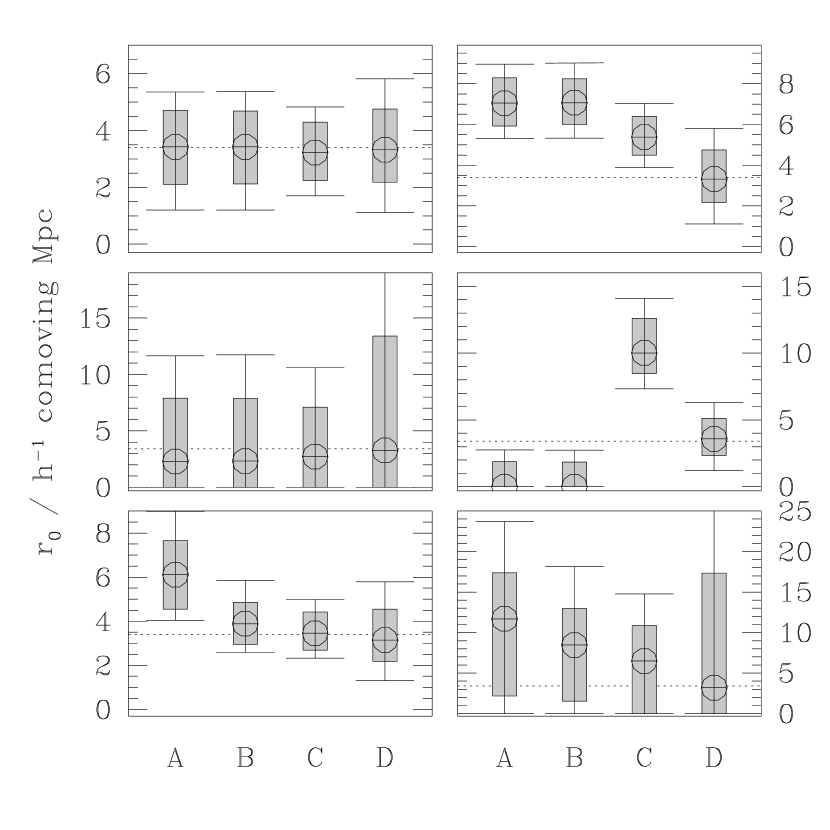
Figure 4: Performance of the 4 methods on simulated galaxy surveys. Each panel shows the results for surveys generated with a single parameter combination (§ 5). Points labeled $A$, $B$, $C$, and $D$ summarize the results for the methods that use equations 1, 4, 5, and 8, respectively. (Equation 1 was actually used in its correctly normalized form, equation A16.) All fits assumed a correlation function slope $\gamma=1.6$ and adopted $\ell=20h^{-1}$Mpc as the maximum pair separation. The circle marks the median estimate of $r_{0}$; the estimates fell within the shaded region for 68% of the simulated surveys, and within the error bars for 90%. The horizontal dashed line shows the true value of $r_{0}$, calculated by counting the number of pairs as a function of separation for all halos in the GIF catalog, then fitting a power-law correlation function to the result. The upper left panel is for a survey with $N=200$ galaxies in a single $10^{\prime}\times 10^{\prime}$ field where the true selection function (a Gaussian with $\mu_{z}=2.2$, $\sigma_{z}=0.35$) is used in the analysis. Survey parameters are varied in other panels. Middle left: $N=20$. Bottom left: spectroscopic selection effects concentrate the survey galaxies near the center of the field. Upper right: a selection function with incorrect width ($\sigma_{z}=0.5$) is used in the analysis. Middle right: a selection function with incorrect mean ($\mu_{z}=2.8$) is used in the analysis. Bottom right panel: $N=20$, angular selection effects, incorrect selection function used in the analysis. Further details are given in § 5.

The results are summarized in Figure 4. All panels are for a simulated survey with a $10^{\prime}\times 10^{\prime}$ field of view. The correlation function slope was fixed to $\gamma=1.6$ and $\ell=20h^{-1}$ Mpc was taken as the maximum pair separation. The panel on the upper left shows the distribution of estimated $r_{0}$ from the four techniques when the pencil beam surveys included $N_{\rm gal}=200$ galaxies each and had a Gaussian selection function with mean $\mu_{z}=2.2$ and r.m.s. $\sigma_{z}=0.35$. I used the correct selection function in calculating $r_{0}$ for the idealized case of this panel, even though normally $r_{0}$ will be calculated from an assumed selection function that is at least somewhat incorrect. This panel provides a reference against which the others can be judged.

The catalogs for the other panels were constructed in the same way, except as noted below. The middle left panel shows the effect of lowering $N_{\rm gal}$ from 200 to 20. The noise in $r_{0}$ increases significantly with catalogs so small. The estimates become biased because the dependence of $r_{0}$ on the number of pairs $n$ is no longer approximately linear over the plausible range of $n$. Although no approach performs particularly well, the method of equation 8 is essentially unusable. This is because random fluctuations in pair counts often make $n_{\rm obs}(0,\ell)=n_{\rm obs}(0,2\ell)$, and the equivalent relationship for $n_{\rm exp}$ requires $r_{0}\to\infty$. (More formally, it is because equation 7 is no longer a good approximation.)

For the bottom left panel, the simulated galaxies’ angular positions were concentrated towards the center of the field rather than being random: each galaxy’s selection probability was multiplied by a Gaussian with $\sigma=70^{\prime\prime}$ centered in the middle of the field, causing 90% of the galaxies in a typical catalog to fall within a region of diameter $5^{\prime}$ inside the larger $10^{\prime}\times 10^{\prime}$ field. This was intended to mimic the sort of selection effect than can appear in multislit spectroscopic surveys. In this case equation 1 leads to biased results, since it makes incorrect assumptions about the galaxies’ angular positions, while the three approaches of § 4 are nearly unaffected.

The upper right panel shows the what happens to the inferred value of $r_{0}$ if the expected pair counts are calculated under the erroneous assumption that the selection-function width is $\sigma_{z}=0.5$. (In all panels its true value is $\sigma_{z}=0.35$.) Equations 1 and 4 fare the worst, producing estimates of $r_{0}$ that are two high by a factor of two. Equation 5 leads to smaller errors, but only because $\sigma_{z}$ was overestimated; for underestimates it performs worse. Only equation 8 yields unbiased results.

The middle right panel shows what happens when the assumed selection function has the correct width $\sigma_{z}=0.35$ but the incorrect mean, $\mu_{z}=2.8$, instead of the true value $\mu_{z}=2.2$. Equations 1 and 4 produce underestimates of $r_{0}$, because the selection function is assumed to be narrower in comoving units than it actually is. Equation 5 produces an overestimate, doing more harm than good in its mangled attempts to compensate for the alignment of the selection function with redshift spikes. Equation 8 remains satisfactory.

The bottom right panel shows a worst case scenario, which may be closer than any other panel to actual cases found in the literature. The sample size is $N_{\rm gal}=20$, the data are subject to angular selection effects (modeled by a two dimensional Gaussian distribution that has $90$% of sources within a region of diameter $7.2^{\prime}$), and the pair counts have been analyzed under the assumption that $\mu_{z}=2.2$, $\sigma_{z}=0.5$ even though the true selection function has $\mu_{z}=2.2$, $\sigma_{z}=0.35$. The results here are so uncertain and biased as to be useless. Estimates $r_{0}>10h^{-1}$ Mpc appear alarmingly often, compensated only by the common occurence of $r_{0}=0$. Adopting equation 4 or 5 helps reduce the noise, but none of the approaches are likely to add significantly to the observer’s prior knowledge of $r_{0}$.

6 UNCERTAINTIES

Equation 2 produces a reasonable estimate of the uncertainty in the simulation results if the “Poisson” uncertainty $n_{\rm obs}^{1/2}$ is replaced with the true uncertainty ${\rm Var}(n_{\rm obs})^{1/2}$, where ${\rm Var}(n)$ is short-hand for the variance of $n$. As Figure 5 shows, the two can differ significantly; the clustering of galaxies drives the variance in pair counts far above the Poisson value ${\rm Var}(n)=n$.

The variance of $n_{\rm obs}$ is easy to estimate for the ensemble of simulated surveys. As long as random errors dominate over cosmic variance, it can be estimated in real life by splitting a survey into many smaller subsamples, calculating the dispersion in $n_{\rm obs}$ among the subsamples, measuring how the dispersion changes with subsample size, and extrapolating to the full sample size. Sample results are shown in Figure 5. For the Lyman-break survey, this approach leads to an estimated $1\sigma$ uncertainty in $r_{0}$ of $\sim 1.3h^{-1}$ Mpc, which agrees well with the value $\sigma_{\rm ftf}/N^{1/2}\simeq 1.1h^{-1}$ Mpc implied by the field-to-field fluctuations $\sigma_{\rm ftf}$ in the estimated value of $r_{0}$ from the $N=15$ individual survey fields.

The preceding discussion applies to values of $r_{0}$ estimated from equations 1, 4, and 5, since in these cases $r_{0}$ is estimated by setting $n_{\rm obs}=n_{\rm exp}$. The uncertainties are slightly more difficult to estimate in the case of equation 8. One approach, in this case, is to estimate the dispersion in $r_{0}$, not $n_{\rm obs}$, among the subsamples, and extrapolate this to the full sample size.

These procedures do not work well for small samples, but neither do the methods for estimating $r_{0}$ itself. I discuss this further in the summary section.

7 SUMMARY

This paper analyzed a method that has recently been used to estimate the spatial clustering strength of small galaxy samples. The method is imperfect. The estimate of $r_{0}$ (a) depends sensitively on the assumed selection function (Figure 1), (b) will be biased if the galaxies are not distributed approximated uniformly across the field (Figure 4), and (c) is strongly affected by the positions of galaxy overdensities relative to the peak of the selection function (Figure 3).

I suggested three ways to mitigate these problems and tested my suggestions on simulated galaxy surveys and on the Lyman-break survey. Figure 4 provides a useful overview of the results. When there are no systematic errors, equation 5 produces the best estimates of $r_{0}$ and equation 8 the worst. Equation 8 is robust against systematic errors, however, and continues to produce reasonable estimates in the presence of systematic effects that render the other approaches useless. Since the approaches respond differently to systematic and random errors, a sensible strategy is to estimate $r_{0}$ with all of them and look for consistency among the results.

The sample analysis of the Lyman-break survey helps illustrate the paper’s main points. An initial estimate of $r_{0}\sim 11h^{-1}$ Mpc from equation 1 disagreed badly with the estimate $r_{0}\sim 4h^{-1}$ Mpc from the robust equation 8, suggesting that the initial analysis must have had large systematic errors. The largest systematic error came from inaccuracies in the assumed selection function. Replacing it with a better model reduced the estimated values of $r_{0}$ to $7.2$, $6.4$, $5.7$, and $4.0h^{-1}$ Mpc from equations 1, 4, 5, and 8, respectively. The differences were still not negligible compared to the random uncertainties (§ 6). The high value from equation 1 was due to artificial angular clustering of galaxies imposed by the survey’s spectroscopic selection criteria. It alone among the estimators does not correct for this. The remaining systematic problems are not easy to trace. They could result from residual errors in the selection function or from changes in the correlation function slope at large separations. In any case, since the effect of systematic errors is minimized when they are small compared to the signal, I maximized the signal by limiting the analysis to angular pairs with smaller separations. As equation 3 shows, the number of pairs with large angular separations is more sensitive to low level systematics than to the clustering strength $\bar{\xi}$. Restricting the analysis to pairs with angular separation $\theta_{ij}<300^{\prime\prime}$, I obtained the estimates $r_{0}=5.1h^{-1}$, $4.9h^{-1}$, $4.4h^{-1}$ Mpc from equations 4, 5, and 8. Since the random uncertainty is $\sim 1h^{-1}$ Mpc (§ 6), these estimates agree well with each other and with the value $r_{0}=4.0\pm 0.6h^{-1}$ Mpc favored by the angular-clustering analysis of Adelberger et al. (2004).

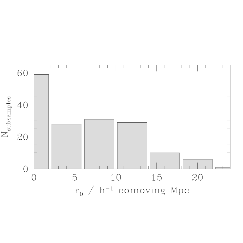
Figure 6: Distribution of $r_{0}$ for 10-galaxy LBG subsamples extracted at random from the 170-object Westphal catalog of Steidel et al. (2003). Correlation lengths were estimated with the approach of equation 1.

This paper provides some support for the common prejudice against estimates of $r_{0}$ derived from small galaxy samples. The middle left panel of Figure 4 shows how large the random uncertainties are for a simulated sample of $N=20$ galaxies with true correlation length $r_{0}=3.5h^{-1}$ Mpc in a $10^{\prime}\times 10^{\prime}$ pencil-beam survey. Figure 6 may make the point more forcefully. I extracted numerous random subsamples of 10 galaxies from the 170-object Lyman-break galaxy catalog in the Westphal field (Steidel et al. 2003), calculated $r_{0}$ for each subsample with equation 1 using the true LBG selection function, and tabulated the results. The spread in estimated $r_{0}$ is enormous.

In realistic situations, uncertainty in the assumed selection function is likely to be the worst source of systematic error. A skeptic might point out that this uncertainty will probably only be large in the small sample limit, where none of the approaches work well, and that my suggested alternatives are not much of an improvement when the uncertainty in the selection function is small (see, e.g., the upper left panel of Figure 4). This is true to a point, but it would be foolish to reject the $\sim 30$% reduction in random uncertainty that equation 5 provides relative to equation 1. According to Figure 5, a $\sim 30$% decrease in the uncertainty in $r_{0}$ for the LBG sample requires a $\sim 40$% increase in the number of galaxies. Using equation 5 instead of 1 in the analysis is surely easier than requesting, obtaining, and reducing $40$% more data. The methods of § 4 are far from perfect, but they improve significantly on their predecessor.

I would like to thank the Florida Airport cafe in La Serena for its hospitality while the first draft of this paper was being written. My collaborators in the Lyman-break survey encouraged me to share the analysis with a wider audience. This work was supported by a fellowship from the Carnegie Institute of Washington.

Appendix A EXPECTED PAIR COUNTS FOR POWER-LAW CORRELATION FUNCTIONS

We derive three simple results needed in the text. In each case, the notation $P(AB|C)$ stands for the probability that $A$ and $B$ are both true if we know that $C$ is true. According to this notation, $P(z_{1}{\bf\Theta_{1}}|z_{2}{\bf\Theta_{2}})$ is the probability of finding a galaxy at redshift $z_{1}$ and angular position ${\bf\Theta_{1}}$ if we know that there is a galaxy at position $z_{2},{\bf\Theta_{2}}$, and $P(z_{1}{\bf\Theta_{1}})$ is the probability of finding a galaxy at the first position if we know nothing about the positions of other galaxies. We assume that the reduced two-point galaxy correlation function, $\xi$, is an isotropic power-law, $\xi(r)=(r/r_{0})^{-\gamma}$, which implies that

$$P(z_{1}{\bf\Theta_{1}}|z_{2}{\bf\Theta_{2}})=P(z_{1}{\bf\Theta_{1}})[1+(r_{12}/r_{0})^{-\gamma}]$$ (A1)

where $r_{12}$ is the distance between the points specified by $z_{1},{\bf\Theta_{1}}$ and $z_{2},{\bf\Theta_{2}}$. Since the survey selection function does not depend on sky position, $P(z_{1}{\bf\Theta_{1}})=P(z_{1})/\Omega$ where $\Omega$ is the survey’s solid angle and $P(z_{1})$ is the expected redshift distribution for a single object in our survey. We adopt the shorthand $z_{12}\equiv z_{1}-z_{2}$ and $\theta_{12}\equiv|{\bf\Theta_{1}}-{\bf\Theta_{2}}|$, and use the capitalized variable $Z_{12}$ to indicate comoving distance between redshifts $z_{1}$ and $z_{2}$.

A.1 Case 1:

If we know that a galaxy with position $z_{2}$, ${\bf\Theta_{2}}$ has a neighbor at angular position ${\bf\Theta_{1}}$, what is the probability that the neighbor has redshift $z_{1}$? In our notation, we are asking for $P(z_{1}|z_{2}{\bf\Theta_{1}\Theta_{2}})$, which can be derived from the correlation function with elementary probability identities:

$$P(z_{1}|z_{2}{\bf\Theta_{1}\Theta_{2}}) = \frac{P(z_{1}{\bf\Theta_{1}}|z_{2}{\bf\Theta_{2}})}{\int_{0}^{\infty}dz_{1}^{\prime}\,P(z_{1}^{\prime}{\bf\Theta_{1}}|z_{2}{\bf\Theta_{2}})}$$ (A2)

$$\simeq \frac{P(z_{1})[1+\xi(r_{12})]}{1+a(r_{0},\gamma,\theta_{12},z_{2})P(z_{2})}.$$ (A3)

The second equality assumes that the selection function is independent of angular position ${\bf\Theta}$ and is roughly constant over the small radial separations where $\xi$ is significantly larger than 0. It also assumes that $f$ and $g$ (defined in the following sentence) do not change significantly over the same small radial separations. For clarity we adopt the shorthand

$$a(r_{0},\gamma,\theta,z)\equiv r_{0}^{\gamma}[f(z)\theta]^{1-\gamma}g^{-1}(z)\beta(\gamma)$$ (A4)

where $g(z)\equiv c/H(z)$ is the change in comoving distance with redshift, $f(z)\equiv(1+z)D_{A}(z)$ is the change in comoving distance with angle, $D_{A}(z)$ is the angular diameter distance, $\beta(\gamma)\equiv B[1/2,(\gamma-1)/2]$, and $B$ is the beta function in the convention of Press et al. (1992).

The probability that the comoving distance $|Z_{12}|$ between $z_{1}$ and $z_{2}$ will be less than $\ell$ can be derived by integrating equation A3 over the appropriate range of $z_{1}$:

$$P(|Z_{12}|<\ell\,|\,z_{2}\theta_{12}) = \frac{\int_{z_{2}-\ell/g}^{z_{2}+\ell/g}dz_{1}\,P(z_{1}{\bf\Theta_{1}}|z_{2}{\bf\Theta_{2}})}{\int_{0}^{\infty}dz_{1}^{\prime}\,P(z_{1}^{\prime}{\bf\Theta_{1}}|z_{2}{\bf\Theta_{2}})}$$ (A5)

$$\simeq \frac{P(z_{2})[2\ell g^{-1}(z_{2})+a(r_{0},\gamma,\theta_{12},z_{2}){\cal I}(\gamma,{\ell},\theta_{12},z_{2})]}{1+a(r_{0},\gamma,\theta_{12},z_{2})P(z_{2})}$$ (A6)

where ${\cal I}$ is related to the incomplete beta function $I_{x}$ of Press et al. (1992) through

$${\cal I}(\gamma,{\ell},\theta,z)\equiv I_{x}[1/2,(\gamma-1)/2]$$ (A7)

with

$$x\equiv\frac{\ell^{2}}{\ell^{2}+[f(z)\theta]^{2}}.$$ (A8)

A.2 Case 2:

What is the probability that the galaxy pair with known angular separation $\theta_{12}$ has comoving redshift separation $|Z_{12}|<\ell$? The probability that a pair with angular separation $\theta_{12}$ will have redshift separation $z_{12}$ is

$$P(z_{12}|\theta_{12})=\int_{0}^{\infty}dz_{2}\,P(z_{2}|\theta_{12})P(z_{12}|z_{2}\theta_{12}),$$ (A9)

which implies that the pair will have comoving radial separation $|Z_{12}|$ less than $\ell$ with probability

$$P(|Z_{12}|<{\ell}\,|\,\theta_{12}) = \int_{0}^{\infty}dz_{2}P(z_{2})\frac{\int_{z_{2}-\ell/g}^{z_{2}+\ell/g}dz_{1}\,P(z_{1}{\bf\Theta_{1}}|z_{2}{\bf\Theta_{2}})}{\int_{0}^{\infty}dz_{1}^{\prime}\,P(z_{1}^{\prime}{\bf\Theta_{1}}|z_{2}{\bf\Theta_{2}})}$$ (A10)

$$\simeq \int_{0}^{\infty}dzP^{2}(z)\frac{2{\ell}g^{-1}(z)+a(r_{0},\gamma,\theta_{12},z){\cal I}(\gamma,{\ell},\theta_{12},z)}{1+a(r_{0},\gamma,\theta_{12},z)P(z)}.$$ (A11)

A.3 Case 3:

What is the expected number of pairs with $|Z_{ij}|<\ell$ if we know only that $N$ galaxies lie somewhere in the solid angle angle $\Omega$? If $I_{i}$ represents the proposition that galaxy $i$ lies within the surveyed solid angle $\Omega$, the expected number of pairs will depend on $\int_{-\ell}^{\ell}dZ_{12}P(Z_{12}|I_{1}I_{2})$, the probability that a randomly selected pair in the survey has comoving redshift separation less than $\ell$. The conditional probability can be rewritten as

$$P(Z_{12}|I_{1}I_{2})=\frac{P(Z_{12}I_{1}I_{2})}{\int_{-\infty}^{\infty}dZ_{12}P(Z_{12}I_{1}I_{2})}$$ (A12)

and the unconditional probability can be expanded to

$$P(Z_{12}I_{1}I_{2})=\int d{\bf\Theta_{1}}d{\bf\Theta_{2}}dz_{2}\,P(Z_{12}{\bf\Theta_{1}}{\bf\Theta_{2}}I_{1}I_{2}z_{2})$$ (A13)

where the integrals in equation A13 extend over all space. If ${\bf\Theta_{1}}$ is not within $\Omega$, $P(Z_{12}{\bf\Theta_{1}}{\bf\Theta_{2}}I_{1}I_{2}z_{2})$ will be equal to 0. If ${\bf\Theta_{2}}$ is within $\Omega$, $P(Z_{12}{\bf\Theta_{1}}{\bf\Theta_{2}}I_{1}I_{2}z_{2})$ will be equal to $P(Z_{12}{\bf\Theta_{1}}{\bf\Theta_{2}}I_{2}z_{2})$ for the same reason that the probability of being in the Louvre and in France is equal to the probability of being in the Louvre. Since the same arguments apply to ${\bf\Theta_{2}}$ and $I_{2}$, equation A13 can be simplified by omitting $I_{1}$ and $I_{2}$ from the right-hand side and restricting the angular integrals to the region $\Omega$. After expanding the integrand with the identify $P(AB)=P(A|B)P(B)$, equation A13 becomes

$$P(Z_{12}I_{1}I_{2})=\int_{\Omega}d{\bf\Theta_{1}}d{\bf\Theta_{2}}\int_{0}^{\infty}dz_{2}P(Z_{12}{\bf\Theta_{1}}|z_{2}{\bf\Theta_{2}})P(z_{2}{\bf\Theta_{2}}).$$ (A14)

The expected number of pairs with $|Z_{12}|<\ell$ is equal to the number of unique pairs multiplied by the probability that a random pair has $|Z_{12}|<\ell$. Substituting equation A14 into equation A12 and integrating over $Z_{12}$, one finds

$$n_{\rm exp} = \frac{N(N-1)}{2}\frac{\int_{\Omega}d{\bf\Theta_{1}}d{\bf\Theta_{2}}\int_{0}^{\infty}dz_{2}\,P(z_{2})\int_{z_{2}-\ell/g}^{z_{2}+\ell/g}dz_{1}\,P(z_{1})[1+\xi(r_{12})]}{\int_{\Omega}d{\bf\Theta_{1}}d{\bf\Theta_{2}}\int_{0}^{\infty}dz_{2}\,P(z_{2})\int_{0}^{\infty}dz_{1}\,P(z_{1})[1+\xi(r_{12})]}$$ (A15)

$$= \frac{N(N-1)}{2}\frac{\int_{\Omega}d{\bf\Theta_{1}}d{\bf\Theta_{2}}\int_{0}^{\infty}dz\,P^{2}(z)[2\ell g^{-1}(z)+a{\cal I}]/\Omega^{2}}{1+r_{0}^{\gamma}\beta(\gamma)\int_{\Omega}d{\bf\Theta_{1}}d{\bf\Theta_{2}}\theta_{12}^{1-\gamma}\int_{0}^{\infty}dz\,P^{2}(z)f^{1-\gamma}(z)g^{-1}(z)/\Omega^{2}}$$ (A16)

which recovers equation 1, aside from the latter equation’s imprecise normalization.

Figure 1: Dependence of the best-fit correlation length in § 2 on the assumed selection function width $\sigma_{\rm sel}$. The point shows the result if $\sigma_{\rm sel}$ is assumed to be $0.4$ exactly. In fact $\sigma_{\rm sel}$ will always be somewhat uncertain, and this is one reason that Poisson error-bars (shown on the point, and derived from equation 2) underestimate the true uncertainty.

Figure 2: The probability that two galaxies will have comoving radial separation $Z_{12}<20h^{-1}$ Mpc as a function of the angle $\theta_{12}$ between them. The actual Lyman-break galaxy selection function (see Figure 3) was used in calculating these numbers. The probability of having small redshift separations depends at least as much on the galaxies’ angular separations as on their correlation length. This implies that angular separations should be treated carefully when estimating $r_{0}$ from the number of redshift pairs.

Figure 5: Dependence of the variance of pair-counts on the number of pairs. Results are shown for Lyman-break galaxies (filled circles) and for halos in the GIF simulation (open squares). To estimate the dependence for LBGs, we created numerous subsamples with different mean numbers of galaxies by eliminating a random fraction of galaxies from the actual LBG catalogs described in § 2. Seven sets of subsamples were created, with the eliminated fraction $f=0.98$, 0.95, 0.9, 0.8, 0.7, 0.6, and 0.5. The point with $n_{\rm obs}\simeq 10^{2.8}$, ${\rm Var}(n_{\rm obs})\simeq 10^{3.6}$ shows the mean and variance of the number of galaxy pairs with radial separation $Z_{12}<20h^{-1}$ Mpc in the subsamples with $f=0.5$. The other points are defined similarly. Each GIF point (open square) shows $\langle n\rangle$ and the variance in $n$ for the ensemble of simulated pencil-beam surveys created for a single set of mock survey parameters (§ 5). These parameter sets include but are not limited to the ones shown in Figure 4. The “Poisson” approximation ${\rm Var}(n)=n$ (solid line) is poor for all values of $n_{\rm obs}$. A better approximation, for the LBG survey, is ${\rm Var}(n)=1.56n^{1.24}$ (dotted line). Different relationships will hold for different surveys, as the GIF results show, and this relationship should not assumed in other situations. A sensible way to estimate ${\rm Var}(n)$ for other surveys is to create random subsamples like these, fit a function to the curve of ${\rm Var}(n)$ vs. $n$, and extrapolate to the observed number of pairs.

References

- (1) Adelberger, K.L. et al. 2004, ApJ, in press
- (2) Blain, A.W., Chapman, S.C., Smail, I., & Ivison, R. 2004, ApJ, in press (astro-ph/0405035)
- (3) Daddi, E. et al. 2002, A&A, 384, L1
- (4) Daddi, E. et al. 2004, ApJL, 600, L127
- (5) Frenk, C.S. et al. 2000, astro-ph/0007362
- (6) Jenkins, A., Frenk, C.S., Pearce, F.R., Thomas, P.A., Colberg, J.M., White, S.D.M., Couchman, H.M.P., Peacock, J.A., Efstathiou, G., & Nelson, A.H., 1998, ApJ, 499, 20
- (7) Kauffmann, G., Colberg, J.M., Diafero, A., & White, S.D.M., 1999, MNRAS, 303, 188
- (8) Press, W. H., Flannery, B. P., Teukolsky, S. A., & Vetterling, W. T. 1992, “Numerical Recipes in C”, (Cambridge: Cambridge University Press)
- (9) Steidel, C.C., Adelberger, K.L., Shapley, A.E., Pettini, M., Dickinson, M., & Giavalisco, M. 2003, ApJ, 592, 728